Accurate simulation estimates of cloud points of polydisperse fluids

Abstract

We describe two distinct approaches to obtaining cloud point densities and coexistence properties of polydisperse fluid mixtures by Monte Carlo simulation within the grand canonical ensemble. The first method determines the chemical potential distribution $\mu(\sigma)$ (with $\sigma$ the polydisperse attribute) under the constraint that the ensemble average of the particle density distribution $\rho(\sigma)$ matches a prescribed parent form. Within the region of phase coexistence (delineated by the cloud curve) this leads to a distribution of the fluctuating overall particle density $n$, $p(n)$, that necessarily has unequal peak weights in order to satisfy a generalized lever rule. A theoretical analysis shows that as a consequence, finite-size corrections to estimates of coexistence properties are power laws in the system size. The second method assigns $\mu(\sigma)$ such that an equal peak weight criterion is satisfied for $p(n)$ for all points within the coexistence region. However, since equal volumes of the coexisting phases cannot satisfy the lever rule for the prescribed parent, their relative contributions must be weighted appropriately when determining $\mu(\sigma)$. We show how to ascertain the requisite weight factor operationally. A theoretical analysis of the second method suggests that it leads to finite-size corrections to estimates of coexistence properties which are exponentially small in the system size. The scaling predictions for both methods are tested via Monte Carlo simulations of a novel polydisperse lattice gas model near its cloud curve, the results showing excellent quantitative agreement with the theory.

I Introduction and background

Examples of polydisperse fluids arise throughout soft matter science, notably in colloidal dispersions, polymer solutions and liquid-crystals. Typically the polydispersity of such systems is manifest as variation in some attribute such as particle size, shape or charge, which is customarily denoted by a continuous parameter $\sigma$. The state of the system is then quantifiable in terms of a distribution $\rho(\sigma)$ measuring the number density of particles of each $\sigma$; more precisely, $\rho(\sigma)d\sigma$ is the number density of particles in the range $\sigma\ldots\sigma+d\sigma$. As such, one can regard the system as a mixture of an infinite number of particle “species” each labelled by the value of $\sigma$ SALACUSE .

As has long been appreciated, polydispersity can profoundly influence the thermodynamical and processing properties of complex fluids LARSON99 ; CHAIKIN00 , making a clear elucidation of its detailed role a matter of both fundamental and practical importance. In particular the phase behaviour of polydisperse systems is known to be considerably richer in both variety and character than that of corresponding monodisperse systems (see e_g_my_review for a recent review). The source of this richness can be traced to fractionation effects: at coexistence a polydisperse fluid described by some initial “parent” distribution, $\rho^{(0)}(\sigma)$, may divide into two or more “daughter” phases $\rho^{(a)}(\sigma)$, $a=1,2,...$, each of which differs in composition from the parent. The sole constraint is that the volumetric average of the daughter distributions equals the parent distribution.

The occurrence of fractionation can engender dramatic alterations to phase diagrams. Insight into the essential features of polydisperse phase behaviour can be gained by first considering the simpler case of a binary mixture of two components whose densities we denote $\rho_{1}$ and $\rho_{2}$ (see also Ref. e_g_my_review ). Let us confine our attention to the case of a “dilution line” in the full phase diagram, in which we vary (at some fixed temperature) the overall (parent) density $n^{(0)}=\rho_{1}^{(0)}+\rho_{2}^{(0)}$, whilst holding constant the ratio of the densities $\rho_{1}^{(0)}/\rho_{2}^{(0)}$, i.e. the overall composition. These parents thus lie on a straight line through the origin in the $(\rho_{1},\rho_{2})$-plane, as shown in fig. 1(a). So-called cloud points (marked A and B) delimit the range of parent densities for which phase coexistence occurs on the dilution line. At cloud point A, the low density parent phase coexists with an infinitesimal volume of a high density daughter phase A’; while at cloud point B, the parent coexists with an infinitesimal volume of a low density daughter phase B’. Owing to fractionation, however, the compositions $\rho_{1}^{(a)}/\rho_{2}^{(a)}$ $(a=1,2)$ of the incipient daughter or “shadow” phases differ in general from that of the parent: the shadow points (A’ and B’) lie off the dilution line.

Figure 1: Schematic representation of the fractionation behaviour of a binary fluid mixture, as described in the text. The parent densities $\rho^{(0)}_{1},\rho^{(0)}_{2}$ are constrained to the dilution line (dashed curve). The curved line indicates the boundary of the coexistence region; straight tielines connect coexisting phases. (a) At the cloud points A and B, the parent phase coexists with the shadow phase A’ and B’ respectively. (b) For a general parent density C in the coexistence region, two daughter phases C’ and C” form. The parent lies on the tieline connecting them; this is the geometrical representation of the lever rule.

For parents on the dilution line but with densities $n^{(0)}$ intermediate between the cloud points (e.g. point C of fig. 1(b)), two daughter phases (C’ and C”) form. These phases occupy finite fractional volumes and their compositions $\rho^{(a)}_{1}/\rho^{(a)}_{2}$ $(a=1,2)$ both differ from that of the parent. Moreover, the daughter phase compositions vary non-trivially as one scans the parent density $n^{(0)}$ between the cloud points. Consequently, and as a result of the lever rule $(1-\xi)\rho^{(1)}_{i}+\xi\rho^{(2)}_{i}=\rho^{(0)}_{i}$ ($i=1,2$), the fractional volumes $1-\xi$ and $\xi$ of two phases will in general depend non-linearly on the parent density. To fully specify the coexistence properties, one thus needs to determine the variation of $\xi$ and $\rho^{(a)}_{1}/\rho^{(a)}_{2}$ $(a=1,2)$ with $n^{(0)}$.

Turning now to the fully polydisperse case, we consider a family of parent density distributions $\rho^{(0)}(\sigma)=n^{(0)}f^{(0)}(\sigma)$ with fixed (normalized) particle size distribution $f^{(0)}(\sigma)$ and varying overall number density $n^{(0)}$, the value of which parameterizes the location of the system on the dilution line. Repeating the above considerations for a range of temperatures, one finds that the familiar liquid-vapor binodal in the density-temperature plane of a monodisperse fluid splits into cloud and shadow curves e_g_my_review , as shown schematically in fig. 2. These mark, respectively, the density of the onset of phase separation and the density of the incipient (shadow) phase NOTE0 . The critical point no longer occurs at the maximum of the cloud curve but at the intersection of the cloud and shadow curves (at which both coexisting phases are identical). One interesting implication of this is that even at the critical temperature, liquid vapor coexistence can occur provided the overall parent density is less than its critical value.

Figure 2: A schematic fluid-fluid phase diagram for a polydisperse fluid, showing temperature $T$ against density; the cloud curve gives the parent density $n^{(0)}$ where phase separation first occurs while the shadow curve records the density of the incipient coexisting phases.

In this work we address the problem of accurately determining phase coexistence properties or, more specifically, cloud point densities of polydisperse mixtures via Monte Carlo (MC) simulation. In a monodisperse system, this task is relatively straightforward (see e.g. Ref. WILDING95 ), because the properties of the coexisting phases at a given temperature are the same for all values of the overall density lying within the coexistence region (as delineated by the binodal). By contrast, for multicomponent fluids, the occurrence of fractionation implies (as we have seen) that the compositions of the phases vary across the coexistence region (i.e. as a function of parent density $n^{(0)}$) and one needs to consider carefully the repercussions of this for simulation estimates of coexistence properties.

The layout of our paper is as follows. In the following section we describe the principal computational issues arising from fractionation and detail two distinct strategies for locating cloud point densities within a grand canonical ensemble framework. The finite-size scaling properties of both methods are analyzed theoretically by generalizing to polydisperse systems scaling concepts developed originally in the context of monodisperse phase equilibria. The predictions for both methods are tested in sec. III via detailed MC simulations of a novel polydisperse lattice gas model. We conclude in sec. IV by comparing and contrasting the relative merits of the two approaches.

II Methods for cloud point determination

We shall work within the grand canonical ensemble (GCE), where the set of chemical potentials $\mu(\sigma)$ is the control parameter, while the particle density $n$ and the particle size distribution are fluctuating variables. (Temperature is assumed held fixed and not written explicitly.) The existence of two phases at given chemical potentials can be detected from the presence of two separate peaks in the probability distribution of the fluctuating order parameter, which we take to be the number density $n$. The fractions $x^{(1)}$, $x^{(2)}$ of probability mass under each of the two peaks of $p(n)$ (i.e. the peak weights) are related to the pressure difference between the two phases as discussed below. For an infinitely large system, where the GCE and the canonical ensemble become equivalent, $x^{(1)}$ and $x^{(2)}$ would correspond to the fractions of overall system volume occupied by each phase, i.e. $1-\xi$ and $\xi$ as defined above.

The density distributions $\rho^{(1)}(\sigma)$, $\rho^{(2)}(\sigma)$ of the two phases can be assigned by averaging only over configurations belonging to either peak of $p(n)$. These are related to the overall average density distribution by

$$\bar{\rho}(\sigma)=x^{(1)}\rho^{(1)}(\sigma)+x^{(2)}\rho^{(2)}(\sigma)\>,$$ (1)

which can be regarded as a generalized form of the lever rule.

In order to estimate the cloud point for the set of dilution line parents $\rho^{(0)}(\sigma)=n^{(0)}f^{(0)}(\sigma)$, one needs to find the value $n^{(0)}_{\rm cl}$ of the parent density $n^{(0)}$ at the boundary of the coexistence region, where the fractional volume of one of the phases, say $x^{(2)}$, drops to zero. Of course, a value of exactly zero is obtained only in the thermodynamic limit of infinite system size; the key question is how a reliable estimate of $n^{(0)}_{\rm cl}$ can nevertheless be extracted from data for finite-sized systems.

II.1 Method A

In method A, proposed originally in WilSolFas05 , we take the natural step of tuning the chemical potentials $\mu(\sigma)$ such that $\bar{\rho}(\sigma)$ from (1) equals directly the parent $\rho^{(0)}(\sigma)$, and measure the density-dependence of the peak weight ratio $r=x^{(2)}/x^{(1)}$. (We do not detail here the algorithm for tuning the $\mu(\sigma)$, which is explained in musig_tuning ). To understand how $r$ will depend on parent density $n^{(0)}$ and system size, note that $r$ is determined by the difference in the grand potential; this is directly related to the pressure $P$ so that $r=\exp(L^{d}\beta\Delta P)$ for large system size $L$. Here $d$ is the dimension of space, $\beta=1/k_{\rm B}T$ and $\Delta P=P^{(2)}-P^{(1)}$. The criterion for stable coexistence is that $r$ must have a finite value as $L\to\infty$; the pressure difference then has to scale as $\Delta P\sim L^{-d}$ except in the special case $r=1$ (see method B below).

For finite $L$, metastable coexistence can still be observed in the density region $n^{(0)}<n^{(0)}_{\rm cl}$ where $\Delta P=O(1)$, but here $r$ will be exponentially small. To estimate $n^{(0)}_{\rm cl}$ from data for a finite system, we use the fact that $\Delta P$ is $O(1)$ and scales linearly with $n^{(0)}-n^{(0)}_{\rm cl}$ to leading order near the cloud point, and hence $\ln r\sim L^{d}(n^{(0)}-n^{(0)}_{\rm cl})$. This applies for $n^{(0)}<n^{(0)}_{\rm cl}$, while above $n^{(0)}_{\rm cl}$ one has $\ln r=O(1)$. Thus the derivative $(\partial/\partial n^{(0)})\ln r$ should drop from an $O(L^{d})$ plateau to $O(1)$ around $n^{(0)}=n^{(0)}_{\rm cl}$. In the second derivative $-(\partial/\partial n^{(0)})^{2}\ln r$ this drop will manifest itself as a peak, whose position serves as an estimate for $n^{(0)}_{\rm cl}$. We next derive the finite-size scaling of the location and shape of this peak.

Our starting point is the rigorous result of BorKot92 for first-order phase transitions driven by some field $h$. The authors of BorKot92 showed that, if the transition is at $h=0$, the free energy density around this point is given by

$$f(h)=-L^{-d}k_{\rm B}T\ln\left(e^{-L^{d}\beta f^{(1)}(h)}+e^{-L^{d}\beta f^{(2)}(h)}\right)$$ (2)

up to exponentially small corrections of order $L^{-d}\exp(-\mbox{const}\times L)$, which can be neglected. The function $f^{(1)}(h)$ ($f^{(2)}(h)$) is the thermodynamic free energy of the first (second) phase in the regime where that phase is stable; elsewhere, i.e. for values of $h$ where the phase would be only metastable in an infinite system, it can be chosen as the continuation with smooth derivatives (up to at least 3rd order BorKot92 ) of the stable free energy. Intuitively, the approximation (2) tells us that the partition function close to the phase transition can be obtained by adding the partition functions of the coexisting (stable or metastable) phases. Formally, it is valid only for values of $|h|\ll L^{-1}$; but in fact we will be interested in rather smaller values of $h\sim L^{-d}\ln L$ where the smaller phase is not yet exponentially suppressed, so that this is not a restriction.

For a polydisperse system within the GCE, the analogue of the field $h$ is the set of chemical potentials. Conceptually it is easiest to think first of particle sizes discretized into a large but finite number $M$ of bins; there are then $M$ chemical potentials and densities which we write as vectors ${\bm{\mu}}$ and $\bm{\rho}$, respectively. More precisely, we take ${\bm{\mu}}$ as the difference of the chemical potentials from those at the desired cloud point, so that the latter is located at ${\bm{\mu}}=\bm{0}$. Assuming that the result (2) can be extended to situations with $M$ field variables instead of a single one we have then for the negative grand potential density, which is nothing but the pressure,

$$P({\bm{\mu}})=L^{-d}k_{\rm B}T\ln\left(e^{L^{d}\beta P^{(1)}({\bm{\mu}})}+e^{L^{d}\beta P^{(2)}({\bm{\mu}})}\right)$$ (3)

The single-phase pressures expanded to second order in ${\bm{\mu}}$ read ($a=1,2$)

$$P^{(a)}({\bm{\mu}})=P_{\rm cl}+\bm{\rho}^{(a)}_{\rm cl}\cdot{\bm{\mu}}+\frac{1}{2}{\bm{\mu}}\cdot\bm{\chi}^{(a)}{\bm{\mu}}$$ (4)

Here $P_{\rm cl}$ is the coexistence pressure at the cloud point, which is common to both phases, while $\bm{\rho}^{(1)}_{\rm cl}$ and $\bm{\rho}^{(2)}_{\rm cl}$ are the (vectors of) particle densities at the cloud point; $\bm{\rho}^{(1)}_{\rm cl}$ is then equal to the parent density vector $\bm{\rho}^{(0)}_{\rm cl}$ at the cloud point, while $\bm{\rho}^{(2)}_{\rm cl}$ is the shadow density vector. The matrices $\bm{\chi}^{(a)}=\nabla_{\bm{\mu}}\bm{\rho}^{(a)}=\nabla_{\bm{\mu}}\nabla_{\bm{\mu}}P^{(a)}$ are the susceptibilities of the particle densities to chemical potential changes, again evaluated at the cloud point.

Taking the chemical potential derivative of (3) we have for the overall density vector

$$\bar{\bm{\rho}}=\frac{\nabla_{\bm{\mu}}P^{(1)}({\bm{\mu}})e^{L^{d}\beta P^{(1)}({\bm{\mu}})}+\nabla_{\bm{\mu}}P^{(2)}({\bm{\mu}})e^{L^{d}\beta P^{(2)}({\bm{\mu}})}}{e^{L^{d}\beta P^{(1)}({\bm{\mu}})}+e^{L^{d}\beta P^{(2)}({\bm{\mu}})}}$$ (5)

This is of the form (1) with the natural correspondences $\bm{\rho}^{(a)}({\bm{\mu}})=\nabla_{\bm{\mu}}P^{(a)}({\bm{\mu}})$, $x^{(1)}=1/(1+r)$, $x^{(2)}=r/(1+r)$ and $\ln r=L^{d}\beta[P^{(2)}({\bm{\mu}})-P^{(1)}({\bm{\mu}})]$. We now expand near the transition, keeping terms to the same order as in (4). With the abbreviations $\Delta\bm{\rho}_{\rm cl}=\bm{\rho}^{(2)}_{\rm cl}-\bm{\rho}^{(1)}_{\rm cl}$ and $\Delta\bm{\chi}=\bm{\chi}^{(2)}-\bm{\chi}^{(1)}$ and using that method A imposes $\bar{\bm{\rho}}=n^{(0)}\mathbf{f}^{(0)}$, where $\mathbf{f}^{(0)}$ is the normalized parent size distribution, one has

$$n^{(0)}\mathbf{f}^{(0)} = \bm{\rho}^{(1)}_{\rm cl}+\bm{\chi}^{(1)}{\bm{\mu}}+\frac{r}{1+r}(\Delta\bm{\rho}_{\rm cl}+\Delta\bm{\chi}{\bm{\mu}})$$ (6)

$$\ln r = L^{d}\beta(\Delta\bm{\rho}\cdot{\bm{\mu}}+{\bm{\mu}}\cdot\Delta\bm{\chi}{\bm{\mu}})$$ (7)

After eliminating ${\bm{\mu}}$, these relations determine the dependence of $r$ on $n^{(0)}$ that we seek. To make progress, we anticipate that the peak in the second derivative $-(\partial/\partial n^{(0)})^{2}\ln r$ will occur at a point where $r=O(L^{-d})$. From (7) this implies that ${\bm{\mu}}=O(L^{-d}\ln L)$ is also small. Keeping only leading order terms in the small quantities $r$ and ${\bm{\mu}}$ and using that $\bm{\rho}^{(1)}_{\rm cl}=n^{(0)}_{\rm cl}\mathbf{f}^{(0)}$, our previous relations then become

$$(n^{(0)}-n^{(0)}_{\rm cl})\mathbf{f}^{(0)} = \bm{\chi}^{(1)}{\bm{\mu}}+r\Delta\bm{\rho}_{\rm cl}$$ (8)

$$\ln r = L^{d}\beta\Delta\bm{\rho}_{\rm cl}\cdot{\bm{\mu}}$$ (9)

Solving the first for ${\bm{\mu}}$ and inserting into the second then gives

$$\ln r=L^{d}\beta\Delta\bm{\rho}_{\rm cl}\cdot(\bm{\chi}^{(1)})^{-1}[(n^{(0)}-n^{(0)}_{\rm cl})\mathbf{f}^{(0)}-r\Delta\bm{\rho}_{\rm cl}]$$ (10)

To absorb the numerical coefficients and make the parent density dimensionless we define

$$z = arL^{d}$$ (11)

$$\tilde{n}^{(0)} = bL^{d}(n^{(0)}-n^{(0)}_{\rm cl})+\ln(aL^{d})$$ (12)

with

$$a = \beta\Delta\bm{\rho}_{\rm cl}\cdot(\bm{\chi}^{(1)})^{-1}\Delta\bm{\rho}_{\rm cl}$$ (13)

$$b = \beta\Delta\bm{\rho}_{\rm cl}\cdot(\bm{\chi}^{(1)})^{-1}\mathbf{f}^{(0)}$$ (14)

The relation (10) then becomes just

$$\tilde{n}^{(0)}=z+\ln z$$ (15)

Differentiating w.r.t. $\tilde{n}^{(0)}$ gives $(\partial/\partial\tilde{n}^{(0)})\ln z=(z+1)^{-1}$ and $-(\partial/\partial\tilde{n}^{(0)})^{2}\ln z=(z+1)^{-2}z\,(\partial/\partial\tilde{n}^{(0)})\ln z=z(z+1)^{-3}$. Bearing in mind that $\ln z$ and $\ln r$ differ only by a constant, we therefore arrive at a universal large-$L$ scaling form for our second-derivative plot

$$-\left(\frac{\partial}{\partial\tilde{n}^{(0)}}\right)^{2}\ln r=\frac{z}{(1+z)^{3}},\quad\tilde{n}^{(0)}=z+\ln z\>$$ (16)

which is parameterized by $z$. All dependence on system details is encoded in the two numerical constants in the definition (12) of the scaled parent density. The curve (16) has its peak at $z=1/2$ so that, from (11), $r$ is $O(L^{-d})$ in the region of interest as anticipated in our derivation. The position of the peak on the horizontal axis is $\tilde{n}^{(0)}=(1/2)-\ln 2$. The scaling (12) then implies that the cloud point estimated from the peak position has finite-size corrections of order $L^{-d}\ln L$, while the peak width and height scale as $L^{-d}$ and $L^{2d}$, respectively. We will find these scalings, and indeed the full shape of the master curve (16), confirmed in the simulation data shown below.

II.2 Method B

While the scaling analysis described above provides a detailed picture of the finite-size corrections that arise when using method A to estimate the location of the cloud point, it would clearly be desirable from a practical point of view to reduce these corrections and ideally make them exponentially small in system size. For monodisperse phase coexistence, this is achieved by measuring the densities of the coexisting phases at the special point where the peaks of $p(n)$ have equal weights $x^{(1)}=x^{(2)}=1/2$, i.e. $r=1$. At this point the pressure difference vanishes. In method A, on the other hand, the pressure difference is $\Delta P=L^{-d}k_{\rm B}T\ln r\sim L^{-d}\ln L$, and this causes the relatively large finite-size corrections. This observation suggests that one should also consider coexisting phases with $r=1$ in the polydisperse case. Of course, one can then no longer require the parent density distribution to equal the overall density distribution in the system, since the latter is an equal mixture of $\rho^{(1)}(\sigma)$ and $\rho^{(2)}(\sigma)$. One has to allow more generally

$$\rho^{(0)}(\sigma)=(1-\xi)\rho^{(1)}(\sigma)+\xi\rho^{(2)}(\sigma)$$ (17)

where $\xi$ is a parameter to be determined; the cloud point is estimated as the parent density at which $\xi$ reaches zero. The results do, however, have physical meaning also for other values of $\xi$ in the range $0\leq\xi\leq 1$: they then provide estimates of properties of the coexisting phases for parent densities $n^{(0)}$ within the coexistence region, with $\xi$ estimating the fractional volume of phase (2). In simple cases, the cloud point $n^{(0)}_{\rm cl}$ could in fact be estimated by linearly extrapolating a few measurements of $\xi(n^{(0)})$ to $\xi=0$. In a monodisperse system this would be exact since $\xi(n^{(0)})$ varies strictly linearly across the coexistence region. In the polydisperse case, on the other hand, $\xi(n^{(0)})$ is a nonlinear function and can exhibit very significant curvature near the cloud point e_g_my_review ; WilSolFas05 ; SpeSol03a . Linear extrapolation is then unreliable and best avoided in favour of direct determination of the density $n^{(0)}$ where $\xi=0$, as explained above.

We will call this approach “method B”. In practice, it is implemented as follows. A parent density is fixed, along with a trial value of $\xi$. The chemical potentials are then tuned until the density distributions of the two coexisting phases satisfy (17). One measures $r=x^{(2)}/x^{(1)}$; if this deviates from $r=1$, $\xi$ is adapted (e.g. using a bisection method) and the process is iterated until $r=1$ to numerical accuracy. If a solution with $0<\xi<1$ is found, we are in the coexistence region. The parent density is then reduced and the process repeated until $\xi$ drops to zero or no solution with positive $\xi$ can be found.

It is straightforward to adapt the above scaling analysis to show that, within method B, finite-size corrections are indeed exponentially small. The condition (17) with $\xi=0$ together with $r=1$ gives as the analogues of (8,9)

$$(n^{(0)}-n^{(0)}_{\rm cl})\mathbf{f}^{(0)} = \bm{\chi}^{(1)}{\bm{\mu}}$$ (18)

$$0 = L^{d}\beta\Delta\bm{\rho}\cdot{\bm{\mu}}$$ (19)

Solving the first and inserting into the second gives

$$0=(n^{(0)}-n^{(0)}_{\rm cl})L^{d}\beta\Delta\bm{\rho}_{\rm cl}(\bm{\chi}^{(1)})^{-1}\mathbf{f}^{(0)}$$ (20)

which (barring accidental vanishing of the constant factor, equal to $b$ from (14)) is satisfied only for $n^{(0)}=n^{(0)}_{\rm cl}$. Finite-size corrections therefore arise only from terms that we had discarded from the outset in our analysis; these are exponentially small. Note that in a practical implementation it is important that $\xi$ is determined to high accuracy; indeed, the analysis above assumes that there is no error in the value of $\xi$. It is easy to see that, if instead $\xi$ was found only with an accuracy of $O(L^{-d})$, then finite-size corrections of the same order as in method A arise.

To summarize, method B is algorithmically a little more involved than method A because it requires for each parent density an “inner loop” over $\xi$, but compensates for this by producing much smaller finite-size corrections. This it achieves by forcing coexisting phases to have identical pressures. The parameter $\xi$ has to be introduced to ensure that the parent distribution is still obtained as an uneven mixture of the two phases. Note that this is a peculiarity of the polydisperse case: no such parameter is necessary for monodisperse systems since the properties of the coexisting phases are the same everywhere within the coexistence region. In a polydisperse scenario, on the other hand, the coexisting phases do change e_g_my_review , and so it is important that the mixing proportions appropriate to the chosen parent density are maintained.

III Application to a polydisperse lattice gas model

III.1 Model definition

In order to test the predictions for the finite-size scaling properties of the two methods detailed above, we have performed a systematic Monte Carlo simulation study of a novel lattice gas model for a polydisperse fluid. The choice of a lattice-based rather than a continuum model was made on the ground of computational tractability: it permits the study of a larger range of system sizes than is feasible for continuum models. We do not expect the scaling predictions for the cloud point estimates to be affected by the presence, or otherwise, of a lattice.

Our polydisperse lattice gas (PLG) model is defined within the grand canonical ensemble by the hamiltonian:

$$H=-\sum_{ij,\sigma,\sigma^{\prime}}\sigma\sigma^{\prime}c_{i}(\sigma)c_{j}(\sigma^{\prime})-\sum_{i,\sigma}\mu(\sigma)c_{i}(\sigma).$$ (21)

Here $\sigma$ is the particle “species”, whose chemical potential is $\mu(\sigma)$, while $c_{i}(\sigma)$ is the number of particles of species $\sigma$ at site $i$, for which we impose a hard-core constraint such that $\sum_{\sigma}c_{i}(\sigma)=0$ or $1$. The instantaneous density distribution follows as $\rho(\sigma)=L^{-d}\sum_{i}c_{i}(\sigma)$, with $d=3$ in the simulations reported below; $i$ runs over the sites of a periodic lattice $i=1,...,L^{d}$, assumed cubic in this work. The sum in the first term on the right hand side of (21) similarly runs over all pairs $i$,$j$ of nearest neighbor sites, as well as over all combinations of $\sigma$ and $\sigma^{\prime}$.

For a study of this model under conditions of fixed polydispersity, one requires knowledge of the chemical potential distribution $\mu(\sigma)$ corresponding to some prescribed form of the ensemble averaged density distribution $\bar{\rho}(\sigma)$. In the context of method A, one tunes $\mu(\sigma)$ such that $\bar{\rho}(\sigma)=\rho^{(0)}(\sigma)$, while for method B one simultaneously tunes $\mu(\sigma)$ together with the parameter $\xi$ to satisfy (17) and the equal peak weight criterion for $p(n)$. Such tuning can be efficiently achieved by a combination of a non-equilibrium Monte Carlo procedure and histogram extrapolation techniques, as has been described previously elsewhere musig_tuning .

We have studied the dilution line properties for a parent distribution having the Schulz form:

$$f^{(0)}(\sigma)=\frac{1}{Z!}\left(\frac{Z+1}{\bar{\sigma}}\right)^{Z+1}\sigma^{Z}\exp\left[-\left(\frac{Z+1}{\bar{\sigma}}\right)\sigma\right].$$ (22)

The mean value of the distribution $\bar{\sigma}$ defines the unit length, while the parameter $Z$ controls the width of the distribution. We fixed the latter to be $Z=50$, resulting in a dimensionless degree of polydispersity

$$\delta\equiv\frac{\sqrt{\overline{(\sigma-\bar{\sigma})^{2}}}}{\bar{\sigma}}=\frac{1}{\sqrt{Z+1}}\simeq 14\%$$ (23)

Lower and upper cutoffs were imposed on the distribution at $\sigma=0.5$ and $1.4$ respectively, and the distribution was normalized accordingly.

III.2 Simulation results

A determination of the critical point parameters for the PLG model using well-established finite-size scaling methods WILDING95 found the critical temperature to be located at $(n_{c}^{(0)},T_{c})=(0.521(1),1.171(1))$ in reduced units. This is to be compared with the critical parameters of the monodisperse (Ising) lattice gas $(0.5,1.127955)$ LUIJTEN . Thus the inclusion of polydispersity of the form (21) is seen to raise both the critical temperature and the critical density. Moreover it splits the liquid-gas binodal into well separated cloud and shadow curves (cf. fig. 2) in a manner similar to that occurring in continuum fluid models for which polydispersity affects the interparticle interaction strength as well as its range WilSolFas05 ; WilFasSol04 . As a consequence, the critical point lies below the maximum of the cloud curve and phase coexistence can be observed even at $T=T_{c}$, provided that $n^{(0)}<n_{c}^{(0)}$.

In view of this we have adopted the critical temperature as a convenient reference point and have studied coexistence along the dilution line $\rho^{(0)}(\sigma)=n^{(0)}f^{(0)}(\sigma)$ for fixed $T=T_{c}$. This involved performing a series of MC runs starting from the critical density and reducing $n^{(0)}$ in a stepwise fashion. Multiple histogram reweighting techniques were employed to estimate the chemical potential distribution at each successive step, while use of multicanonical preweighting techniques BergNeuh92 ensured that both coexisting phases were efficiently sampled in the course of each simulation run (see ref. WilFasSol04 for a fuller account of this procedure).

The dilution line was scanned in this manner for lattices of sizes $L=10,~{}12,~{}15,~{}18,~{}21$ using both methods A and B. The GCE simulations directly yield the form of $p(n)$ corresponding to either case. For method A, one observes (figs. 3(a) and 3($a^{\prime}$)) that as $n^{(0)}$ is reduced from its critical point value, the peaks in $p(n)$ separate, while the valley between them deepens. This is accompanied by a gradual transfer of weight from the liquid to the gas peak. We extract the ratio of the peak areas at a given $n^{(0)}$ from $p(n)$ via

$$r(n^{(0)})=\frac{\int_{n>n^{*}}p(n)dn}{\int_{n<n^{*}}p(n)dn},$$ (24)

Here $n^{*}$ is a convenient threshold density intermediate between vapor and liquid densities, which we take to be the location of the minimum in $p(n)$.

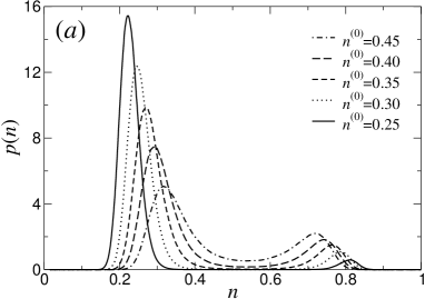
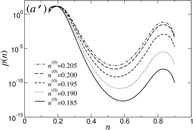
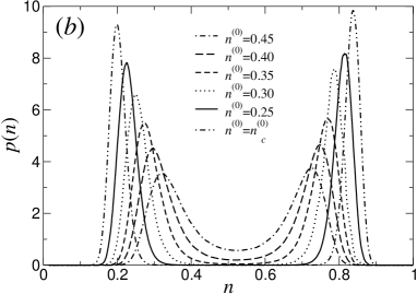
Figure 3: ${\bf(a)}$ Estimates of the form of $p(n)$ for a selection of values of $n^{(0)}$ within the liquid-vapor coexistence region as obtained from the GCE simulation data obtained according to method A. The associated estimates of $r$ are, in order of decreasing $n^{(0)}$: $r=0.4483,0.2682,0.1643,0.0901,0.0379$. ${\bf(a^{\prime})}$ The distributions for a selection of small values of $n^{(0)}$ displayed on a logarithmic scale. ${\bf(b)}$ The corresponding estimates of $p(n)$ obtained according to method B (for which the peak weight ratio is constrained to unity). The associated estimates of $r_{\xi}$ are, in order of decreasing $n^{(0)}$: $r_{\xi}=0.4158,0.2411,0.1477,0.0822,0.0335$. All the plots refer to system size $L=15$.

The form of $p(n)$ obtained using method B is shown in fig. 3(b) for a selection of values of $n^{(0)}$. Here, by virtue of the appropriate tuning of the parameter $\xi$, the vapor and the liquid peaks maintain equal weights throughout the coexistence region. The estimate of the ratio of fractional phase volumes is obtained simply as $r_{\xi}=\xi/(1-\xi)$. We use the subscript $\xi$ here to distinguish this quantity from the probability mass ratio $r$ as extracted from (24), the latter being more directly related to the pressure difference between the phases as explained above.

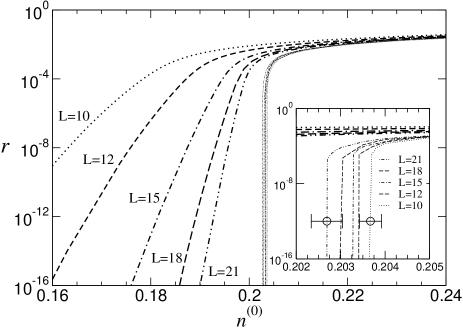
Figure 4: The value of $r$ as estimated from method A (labelled thick curves) and of $r_{\xi}$ from method B (unlabelled, thin curves); both are plotted against parent density $n^{(0)}$. The inset shows in greater detail the results for method B in the vicinity of the cloud point density. An estimate of the statistical errors of the procedure were obtained via a block analysis. The errors for the smallest and largest system size are indicative of the statistical uncertainty of our results.

In fig. 4, we plot the dependence of $r$ on parent density $n^{(0)}$ as obtained from method A for the various system sizes we have studied, alongside the results for $r_{\xi}$ from method B. The curves for method A (thick lines) show a strong $L$-dependence within the metastable coexistence region which borders the cloud point at small $n^{(0)}$. As $n^{(0)}$ is increased, however, and the cloud point is approached, the curves cross over to their $L$-independent limit values in the coexistence region.

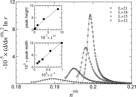
Figure 5: Points show the estimated second derivative $-(\partial/\partial n^{(0)})^{2}\ln r$ obtained within method A. The solid lines superimposed on these data points are scaled fits of the form (16). Insets show the $L$-dependence of the peak width and height plotted in terms of the predicted scaling variable and accompanied by a least squares fit.

Looking in more detail at the finite-size scaling properties of the curves for $r(n^{(0)})$ from method A, the analysis of sec. II.1 shows that the cloud point region is associated with a peak in the second derivative $-(\partial/\partial n^{(0)})^{2}\ln r$. In Fig. 5 we plot this quantity for the various systems sizes studied. Superimposed on each plot is a suitably scaled form of the predicted universal master curve, (16). The non-universal scale factors for the height and the width of the master curves implicit in the fitting shown are plotted in the insets against the predicted scaling variables $L^{2d}$ and $L^{-d}$ respectively (cf. sec. II.1). Clearly there is good agreement with the predictions for both the general shape of the peak and the scaling of its width and height. Some discrepancies between the observed and measured peak shape are apparent on the low density side, well away from the peak maximum, particularly for the smaller system sizes. These are presumably attributable to the breakdown of the validity of the linear expansion in the density difference used in the derivation of (16).

The estimates of $r_{\xi}(n^{(0)})$ deriving from application of method B, as shown in Fig. 4, exhibit a qualitatively different behavior. As the density is increased from the cloud point, one observes a rapid, near-vertical increase in $\ln r_{\xi}$ from a large negative value (where $r_{\xi}$ is essentially zero) to values of $O(1)$. There is only a weak dependence of this behaviour on the system size (see inset of fig. 4). Within this method the cloud point density can thus be directly read off as the lowest density at which an equal-peak-weight solution exists to the numerical procedure described in Sec. II.2. We note that, as expected, $r$ from method A and $r_{\xi}$ from method B converge to similar values for parent densities well within the coexistence region.

Fig. 6 compares for the two methods the finite-size behaviour of the cloud point density estimates. In the case of method A, the estimate for a given $L$ derives from the position of the peak in the second derivative plot (fig. 5). Fig. 6 confirms that (as predicted) these estimates deviate from their limiting value by a correction O$(L^{-d}\ln L)$. A least-square fit yields $n_{\rm cl}^{(0)}=0.20266(12)$ as the best estimate of the cloud point density (see also inset). In the case of method B, the cloud point is estimated as the lowest value of $n^{(0)}$ for which an equal-peak-weight solution for $p(n)$ can be found. The finite-size corrections to this estimate are expected to be exponentially small in the system size and our results (fig. 6(b)) are consistent with this, yielding a cloud point estimate $n_{\rm cl}^{(0)}=0.2028(1)$. Indeed the corrections appear to be so small that even for the smallest system size studied ($L=10$) the estimate of the cloud point density obtained using method B deviates from the limiting value by just $0.5\%$. This compares with a relative deviation of approximately $10\%$ for method A.

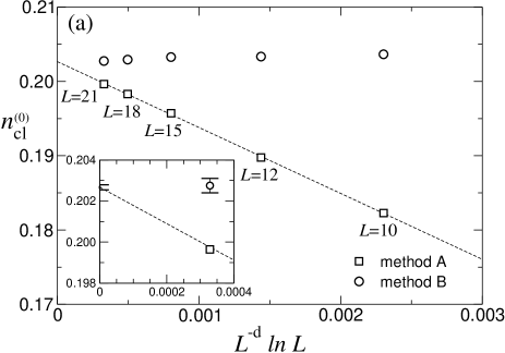
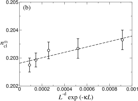
Figure 6: Finite-size scaling of the cloud point estimates deriving from methods A and B. (a) The data for both methods are plotted against the predicted scaling variable for method A. The dashed line is a least squares fit to the estimates from method A and the inset shows a magnified view of the region of large $L$. (b) The estimates deriving from method B, plotted against $L^{-d}\exp(-\kappa L)$ with $\kappa=8.988\times 10^{-3}$. Except where error bars are shown, statistical uncertainties are smaller than the symbol sizes.

IV Conclusions

We summarize. We have presented and tested two distinct finite-size scaling strategies for estimating coexistence properties and cloud points in polydisperse fluids within a grand canonical ensemble framework. Both are, of course, also directly applicable to multicomponent mixtures of many discrete species. The first approach, “method A” takes the natural step of constraining the ensemble average of the density distribution $\rho(\sigma)$ to match the prescribed parent form. However, in order to satisfy the lever rule, this necessarily leads to unequal peak weights in the order parameter distribution function $p(n)$. For systems of finite size, this translates to a finite pressure difference between the coexisting phases, which in turn engenders finite-size corrections to estimates of the cloud point density which are powers of the system size.

The second approach, “method B” strictly imposes equal peak weights for $p(n)$, and hence pressure equality in systems of finite size. The coexistence properties of the desired parent are obtained by appropriately weighting the relative contributions of the coexisting phases to the overall density distribution in such a way that the lever rule is satisfied. We have detailed how to determine this weight factor operationally and shown that method B has finite-size corrections to the coexistence properties which are exponentially small in the system size. As such, and notwithstanding the need to determine the phase weighting factor $\xi$, method B is clearly superior to method A. It can be regarded as a generalization to multicomponent mixtures of the well known equal peak weight criterion BorKot92 developed in the context of monodisperse systems by Borgs and coworkers.

- (1) J.J. Salacuse and G. Stell, J. Chem. Phys. 77, 3714 (1982).
- (2) R.G. Larson, The Structure and Rheology of Complex fluids (Oxford University Press, New York, 1999).
- (3) P. Chaikin in Soft and Fragile Matter, M.E. Cates and M.R. Evans (eds.), IOP publishing, London, 2000.
- (4) P. Sollich, J. Phys. Condens. Matter 14, R79 (2002).
- (5) For each parent density within the cloud curve there is a unique coexistence curve, not shown in fig. 2; see ref. e_g_my_review .
- (6) N. B. Wilding, Phys. Rev. E 52, 602 (1995).
- (7) N.B. Wilding, P. Sollich and M. Fasolo, Phys. Rev. Lett. 95, 155701 (2005).
- (8) N.B. Wilding, J. Chem. Phys. 119, 12163 (2003); N.B. Wilding and P. Sollich, J. Chem. Phys. 116, 7116 (2002).
- (9) C. Borgs and W. Janke, Phys. Rev. Lett. 68, 1738 (1992); C. Borgs and R. Kotecky, Phys. Rev. Lett. 68, 1734 (1992).
- (10) A. Speranza and P. Sollich, J. Chem. Phys. 118, 5213 (2003).
- (11) H.W.J. Bloete, E. Luijten and J.R. Heringa, J. Phys. A 28, 6289 (1995).
- (12) N.B. Wilding, M. Fasolo and P. Sollich, J. Chem. Phys. 121, 6887 (2004).
- (13) B.A. Berg and T. Neuhaus, Phys. Rev. Lett. 68, 9 (1992).