Coherent exciton transport in dendrimers and continuous-time quantum walks

Abstract

We model coherent exciton transport in dendrimers by continuous-time quantum walks (CTQWs). For dendrimers up to the second generation the coherent transport shows perfect recurrences, when the initial excitation starts at the central node. For larger dendrimers, the recurrence ceases to be perfect, a fact which resembles results for discrete quantum carpets. Moreover, depending on the initial excitation site we find that the coherent transport to certain nodes of the dendrimer has a very low probability. When the initial excitation starts from the central node, the problem can be mapped onto a line which simplifies the computational effort. Furthermore, the long time average of the quantum mechanical transition probabilities between pairs of nodes show characteristic patterns and allow to classify the nodes into clusters with identical limiting probabilities. For the (space) average of the quantum mechanical probability to be still or again at the initial site, we obtain, based on the Cauchy-Schwarz inequality, a simple lower bound which depends only on the eigenvalue spectrum of the Hamiltonian.

I Introduction

In recent years dendrimers have been an active field of research, both experimentally and theoretically, see, e.g.  reference Vögtle (1998) or the Special Issue of Journal of Luminescence on the optical properties of dendrimers.jlu (2005) Dendrimers are hyperbranched macromolecules with a very regular structure. Among a series of very interesting and crossdisciplinary applications like drug delivery, dendrimers have been theoretically investigated as light harvesting antennae.Mukamel (1997); Jiang and Aida (1997); Bar-Haim and Klafter (1998); Flomenbom et al. (2005) Apart from these theoretical works, there has been also a huge experimental effort to probe transport processes.Kopelman et al. (1997); Shortreed et al. (1997); Lupton et al. (2001); Varnavski et al. (2002a, b) Here, dendrimers are synthesized in a self-similar fashion by hierarchically growing the dendrimer from a core.Bharathi et al. (1995) Depending on the site of the light absorbing states, the transport of these excitations can be very efficient in some cases but also very inefficient in others. At high temperatures the transport is incoherent and can be described by a hopping process.Shortreed et al. (1997) However, there is also experimental evidence for coherent interchromophore transport processes within the dendrimer.Varnavski et al. (2002a, b) When modeling the transport, one usually assumes that the excitations are localized on the building blocks of the dendrimer, i.e., either on the chromophores or the segments connecting the chromophores. The latter leads to a different topology usually referred to as being a (finite) Husimi cactus.Poliakov et al. (1999)

There is a long-standing study of exciton transport in molecular aggregates, not only in polymer physics Kenkre and Reineker (1982) but also in atomic Shore (1990) and in solid state physics.Davydov (1962); Haken (1976) In solid state physics, a dendrimer of infinite generation is known as the Bethe lattice. The incoherent exciton transport in dendrimers can be efficiently modelled by random walks, see, for instance, Heijs et al. (2004); Vlaming et al. (2005); Blumen et al. (2005). Here, the underlying topology of the dendrimer determines the dynamics of the exciton motion and the transport is described by a master (rate) equation.

In this paper we will consider only the coherent transport, and we will model the dynamics by Schrödinger’s equation. Interestingly, this is formally closely related to the master equation approach, where the transfer over the system is given by the connectivity matrix ${\bf A}$ of the dendrimer,Mülken and Blumen (2005a, b); Mülken et al. (2005); Mülken and Blumen (2006) vide infra. This is also in close relation to Hückel’s (or LCAO, linear combination of atomic orbitals) theory,McQuarrie (1983) where the elements of the secular matrix are given by ${\bf A}$.

II Coherent exciton transport on graphs

We model the coherent transport of excitons on graphs by so-called continuous-time quantum walks (CTQWs) which are the quantum mechanical analog of continuous-time random walks (CTRWs).

A graph is a collection of connected nodes and to every graph there exists a corresponding connectivity matrix ${\bf A}=(A_{ij})$, which is a discrete version of the Laplace operator. The non-diagonal elements $A_{ij}$ equal $-1$ if nodes $i$ and $j$ are connected by a bond and $0$ otherwise. The diagonal elements $A_{ii}$ equal the number of bonds which exit from node $i$, i.e., $A_{ii}$ equals the functionality $f_{i}$ of the node $i$.

Classically, a CTRW is governed by a master equation for the conditional probability, $p_{k,j}(t)$, to find the CTRW at time $t$ at node $k$ when starting at node $j$.Weiss (1994); van Kampen (1990) The transfer matrix of the walk, ${\bf T}=(T_{kj})$, is related to the connectivity matrix by ${\bf T}=-\gamma{\bf A}$, where we assume for simplicity the transmission rate $\gamma$ of all bonds to be equal and we set $\gamma\equiv 1$.

CTQWs are obtained by identifying the Hamiltonian of the system with the (classical) transfer operator (matrix), ${\bf H}=-{\bf T}$.Farhi and Gutmann (1998); Childs et al. (2002); Mülken and Blumen (2005a) The whole accessible Hilbert space is spanned by the basis vectors $|j\rangle$ associated with the nodes $j$ of the graph. A state $|j\rangle$ starting at time $t_{0}$ evolves in time as $|j(t)\rangle={\bf U}(t,t_{0})|j\rangle$, where ${\bf U}(t,t_{0})=\exp(-i{\bf H}(t-t_{0}))$ is the quantum mechanical time evolution operator (we have set $m\equiv 1$ and $\hbar\equiv 1$).

The transition amplitude $\alpha_{k,j}(t)$ from state $|j\rangle$ at time $0$ to state $|k\rangle$ at time $t$ reads then $\alpha_{k,j}(t)=\langle k|{\bf U}(t,0)|j\rangle$ and obeys Schrödinger’s equation. Denoting the orthonormalized eigenstates of the Hamiltonian ${\bf H}=-{\bf T}$ by $|q_{n}\rangle$, such that $\sum_{n}|q_{n}\rangle\langle q_{n}|=\boldsymbol{1}$, the quantum mechanical transition probability is

$$\pi_{k,j}(t)\equiv|\alpha_{k,j}(t)|^{2}=\left|\sum_{n}\langle k|e^{-i\lambda_{n}t}|q_{n}\rangle\langle q_{n}|j\rangle\right|^{2}.$$ (1)

Note that classically $\sum_{k}p_{k,j}(t)=1$, whereas quantum mechanically $\sum_{k}|\alpha_{k,j}(t)|^{2}=1$ holds.

III Topology & connectivity of dendrimers

In the following we will consider dendrimers of generations $G$ whose functionality is $3$, i.e. all internal nodes of the dendrimer have $3$ bonds, whereas the outermost nodes have only one bond. The stucture of such dendrimers is exemplified in Fig. 1 for dendrimers of generations $G=2$ and $G=3$. Note that the number of nodes belonging to the $g$-th generation ($g\geq 1$) is $3\cdot 2^{g-1}$ and that it grows exponentially with $g$. Moreover, the total number of nodes in the dendrimer of generation $G$ is $N=3\cdot 2^{G}-2$.

Figure 1: Dendrimers of generation $G=2$ (left) and $G=3$ (right).

The connectivity matrix of these dendrimers has a very simple structure. One has $A_{ii}=3$ for all the nodes in the first $G-1$ generations and $A_{ii}=1$ for the nodes in generation $G$. The bonds are represented by the off-diagonal matrix elements $A_{ij}$. Here, every node in generation $g\geq 1$ is connected to two consecutively numbered nodes in generation $g+1$ and to one node in generation $g-1$.

The eigenmodes of such dendrimers were studied in.Cai and Chen (1997) There, for the dendrimers of generations $G=1$ and $G=2$, the eigenvalues and eigenvectors of ${\bf A}$ were explicitly calculated. The eigenvectors determine the eigenmodes of the dendrimer, see e.g. Fig. 3 of Cai and Chen (1997). It was further shown that there are $G+1$ nondegenerate eigenvalues, one of which is always $\lambda_{0}=0$. We used these results to check that our numerical diagonalization for the small dendrimers is correct.

IV Transport on dendrimers

In the following section we present results for coherent exciton transport on dendrimers. The results were obtained by numerically determining the eigenvalues and eigenvectors of the corresponding connectivity matrix, using the standard software package MATLAB.

IV.1 Dynamics of an excitation starting at the center

We start by focusing on an excitation which starts at the central node $1$. For a $G=3$ dendrimer, Fig. 2 shows snapshots of the temporal development of transition probabilities. The nodes are numbered according to Fig.1. In this way the nodes $2-4$ belong to generation $g=1$, the nodes $5-10$ to $g=2$, and the nodes $11-22$ to $g=3$. Here, the excitation spreads over the whole dendrimer and already after a short period of time, $t\approx 1.5$, there is a considerable probability to be at the outermost nodes, which is larger than the probabilities to be at nodes belonging to other generations. The initial “speed” of the exciton is calculated based on the number of bonds (i.e. the chemical distance) between the initial node and one of the outermost nodes, divided by the time to reach that node. Here, we have $3/1.5=2$. As we will show below, the dynamics of an excitation starting at the central node $1$ over the dendrimer can be mapped onto a line. For an infinite line, the transition probabilities can be expressed by Bessel functions of the first kind.Mülken and Blumen (2005b) From this the speed can be calculated; it is at all times equal to $2$. For finite lines, the initial speed is still equal to $2$. Thus our results here are in accordance with what can be expected for waves propagating through a regular graph.

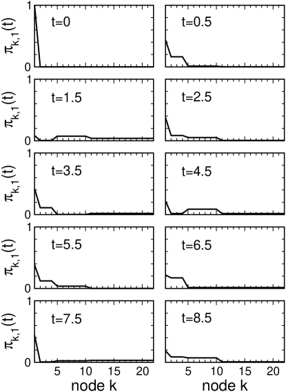
Figure 2: Snapshots of the transition probability for a $G=3$ dendrimer at different times $t$. The initial excitation is at the central node.

Remarkably, for the $G=2$ dendrimer the transition probabilities are fully periodic when the coherent excitation starts from the central node $1$ (the same holds for the $G=1$ dendrimer, too). In this case we obtain, based on the analytically determined eigenvalues and eigenvectors that all $\pi_{k,1}(t)$ have the following, periodic form:

$$\pi_{k,1}(t)=\left|\sum_{n}e^{-i\lambda_{n}t}\langle k|q_{n}\rangle\langle q_{n}|1\rangle\right|^{2}$$

$$=a^{(k)}_{0}+a^{(k)}_{1}\cos(2t)+a^{(k)}_{2}\cos(3t)+a^{(k)}_{3}\cos(5t).$$ (2)

Note that due to rotational symmetry, the transition probabilities from the central node to nodes belonging to the same generation are equal. Because of this we only have to list three different transition probabilities. We hence choose, exemplarily, the nodes $1$, $2$, and $10$, for which we find the coefficients

$$a^{(1)}_{0}=\frac{21}{50}\ ,\ a^{(1)}_{1}=\frac{1}{10}\ ,\ a^{(1)}_{2}=\frac{2}{5}\ ,\ a^{(1)}_{3}=\frac{2}{25}$$

$$a^{(2)}_{0}=\frac{49}{450}\ ,\ a^{(2)}_{1}=\frac{1}{30}\ ,\ a^{(2)}_{2}=-\frac{4}{45}\ ,\ a^{(2)}_{3}=-\frac{4}{75}$$

$$a^{(10)}_{0}=\frac{19}{450}\ ,\ a^{(10)}_{1}=-\frac{1}{30}\ ,\ a^{(10)}_{2}=-\frac{1}{45}\ ,\ a^{(10)}_{3}=\frac{1}{75}.$$

If follows that there is a perfect revival of the initial state for each $t=2n\pi$ where $n\in\mathbb{N}$. At $t=(2n-1)\pi$ the main part of the excitation is equally distributed among the nodes of the outermost generation. This revival of the initial probability distribution resembles results obained for continuous Kinzel (1995); Grossmann et al. (1997) and discrete quantum carpets.Iwanow et al. (2005); Mülken and Blumen (2005b) For discrete quantum carpets, the revival is only perfect for small cycles of length $N=1,2,3,4,$ and $6$. When the cycles become larger, there are only partial revivals of the initial state. The same can be observed for dendrimers of generation $G\geq 3$, as will become clear in the following.

IV.2 Mapping onto a line

Due to the rotational symmetry, the dynamical problem of a dendrimer initially excited at its center $1$ can be mapped onto a linear segment. In the classical, CTRW case, this result has been widely used, see Ref. Bar-Haim and Klafter (1998). For a CTQW on a graph consisting of two Cayley trees this has been done in, e.g., Childs et al. (2002); Mülken and Blumen (2005a). For each generation with $g\geq 1$ we introduce linear combinations of states

$$|g\rangle\equiv\frac{1}{\sqrt{3\cdot 2^{g-1}}}\sum_{k\in g}|k\rangle.$$ (3)

The state of generation $0$, $|g_{0}\rangle$, is identical to that of the central node $|1\rangle$. A CTQW through the generations is now governed by a new Hamiltonian $\tilde{\bf H}$ which is defined by

$$\tilde{H}_{gg^{\prime}}=\langle g|{\bf H}|g^{\prime}\rangle.$$ (4)

Given ${\bf H}$ and the construction of the generation states $|g\rangle$, $\tilde{\bf H}$ is a real and tridiagonal matrix whose elements obey $\tilde{H}_{gg^{\prime}}=\tilde{H}_{g^{\prime}g}$ and are given by

$$\tilde{H}_{gg} = \langle g|{\bf H}|g\rangle=f_{g}\ ,$$ (5)

$$\tilde{H}_{g,g\pm 1} = \langle g|{\bf H}|g\pm 1\rangle=\frac{\sqrt{2^{\mp 1}}}{3\cdot 2^{g-1}}\sum_{k\in g}\sum_{j\in g\pm 1}\langle k|{\bf H}|j\rangle$$ (6)

$$= \begin{cases}-\sqrt{3}&\mbox{for}\quad\tilde{H}_{01}=\tilde{H}_{10}\\ -\sqrt{2}&\mbox{else}.\end{cases}$$

Here, $f_{g}$ is the functionality of the nodes in generation $g$ and all other elements of $\tilde{\bf H}$ are zero. In this way the original eigenvalue problem which grows exponentially with $G$ has been reduced to an eigenvalue problem which grows only linearly with $G$. The $G+1$ eigenvalues of the new matrix $\tilde{\bf H}$ are the nondegenerate eigenvalues of the original matrix ${\bf H}$. In terms of eigenmodes, these are the modes of the full dendrimer, where, in a classical picture,Cai and Chen (1997) nodes belonging to the same generation move in the same direction.

Now, the transition amplitude between different generations can be written as $\langle g|\exp(-i\tilde{\bf H}t)|g_{0}\rangle$ . It is easy to show that the transition probabilities for a line of $3$ nodes obtained from the $G=2$ dendrimer are, see Eq.(2),

$$\left|\langle g|\exp(-i{\bf H}t)|g_{0}\rangle\right|^{2}=\sum_{k\in g}\pi_{k,1}(t).$$ (7)

The cumulative transition probabilities for the $G=2$ and the $G=3$ dendrimer to go from one generation of the dendrimer to another one when starting at $g=0$ are shown in Fig. 3. For generations $G\geq 3$, we do not find perfect revivals of the initial probability anymore.

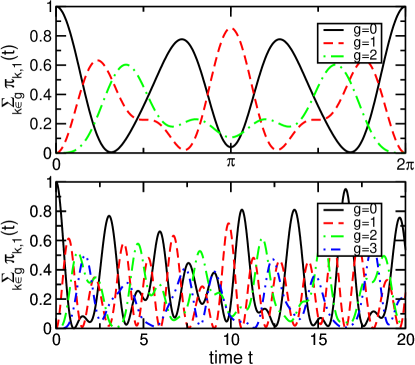
Figure 3: (Color online). Cumulative transition probabilities that a coherent excitation starting at the central node is at time $t$ at a node of generation $g$. We present the situation for dendrimers of generations (a) $G=2$ and (b) $G=3$. Note the complete revival at $t=2\pi$ for the $G=2$ dendrimer.

IV.3 Dynamics of excitations starting off-center

If the initial excitation is placed at one of the nodes of the outermost generation $g=G$ of the dendrimer, the picture changes. Snapshots of the transition probability for a $G=3$ graph where the excitation starts at the outermost node $22$ are shown in Fig. 4. Even classically the propagation through the dendrimer gets to be much slower than in the previous case, see e.g. Bar-Haim et al. (1997); Rana and Gangopadhyay (2003); Heijs et al. (2004). Nevertheless, eventually the excitation will classically propagate through the whole graph and in the long time limit the probability will be equipartitioned among all nodes.

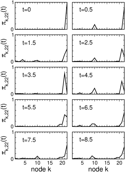
Figure 4: Snapshots of the transition probability for a $G=3$ dendrimer at different times $t$. The excitation starts at the outermost node $22$.

Quantum mechanically this effect is even more dramatic. For the times shown in Fig. 4, the main fraction of $\pi_{k,j}(t)$ stays in a small region closely connected by bonds to the initial node $j$, and the transfer to other sites is highly unlikely. For the $G=3$ dendrimer shown in Fig. 1, the excitation is located with very high probability on the initial node $22$ and on the nodes $21$ and $10$. On the time scales shown in Fig. 4, the probability for nodes outside the branch (consisting of the nodes $1,4,9,10,19,20,21,$ and $22$) to be excited is very low .

As we show in the following section, also at long times the limiting probability for the excitation to reach the other branches of the dendrimer stays very low.

IV.4 Long time limit

Quantum mechanically the temporal development is symmetric to inversion; this prevents $\pi_{k,j}(t)$ from having a definite limit for $t\to\infty$. In order to compare the classical long time probability with the quantum mechanical one, one usually uses the limiting probability (LP) distribution Aharonov et al. (2001)

$$\chi_{k,j}\equiv\lim_{T\to\infty}\frac{1}{T}\int_{0}^{T}dt\ \pi_{k,j}(t),$$ (8)

which can be rewritten by using the orthonormalized eigenstates of the Hamiltonian, $|q_{n}\rangle$, as Mülken et al. (2005)

$$\chi_{k,j} = \lim_{T\to\infty}\frac{1}{T}\int_{0}^{T}dt\ \left|\sum_{n}\langle k|e^{-i{\bf H}t}|q_{n}\rangle\langle q_{n}|j\rangle\right|^{2}$$ (9)

$$= \sum_{n,m}\delta_{\lambda_{n},\lambda_{m}}\langle k|q_{n}\rangle\langle q_{n}|j\rangle\langle j|q_{m}\rangle\langle q_{m}|k\rangle.$$

Some eigenvalues of $\bf H$ might be degenerate, so that the sum in Eq. (9) can contain terms belonging to different eigenstates $|q_{n}\rangle$ and $|q_{m}\rangle$.

We can use the Cauchy-Schwarz inequality Abramowitz and Stegun (1972)

$$\left|\int_{0}^{T}dt\ f(t)g(t)\right|^{2}\leq\left(\int_{0}^{T}dt\ |f(t)|^{2}\right)\left(\int_{0}^{T}dt\ |g(t)|^{2}\right)$$ (10)

to obtain a lower bound for the LP. With $f(t)\equiv\alpha_{k,j}(t)$ and $g(t)\equiv 1$, the time integral in Eq. (8) fulfills the inequality

$$\int_{0}^{T}dt\ |\alpha_{k,j}(t)|^{2}\geq\frac{1}{T}\left|\int_{0}^{T}dt\ \alpha_{k,j}(t)\right|^{2}.$$ (11)

This results in

$$\chi_{k,j}\geq\lim_{T\to\infty}\left|\frac{1}{T}\int_{0}^{T}dt\ \sum_{n}\langle k|e^{-i\lambda_{n}t}|q_{n}\rangle\langle q_{n}|j\rangle\right|^{2}.$$ (12)

The only term in the sum over $n$ in Eq. (12) which survives after integration and taking the limit $T\to\infty$ is the one with $\lambda_{0}=0$. In terms of eigenmodes, the eigenstate corresponding to $\lambda_{0}$ is the one for which in a classical picture the dendrimer moves as a whole in one direction. The corresponding eigenvector can be written as $|q_{0}\rangle=1/\sqrt{N}\sum_{j=1}^{N}|j\rangle$. Since the states $|j\rangle$ form a complete, ortho-normalized basis set, i.e. $\langle k|j\rangle=\delta_{kj}$, we get $\langle k|q_{0}\rangle=\langle q_{0}|j\rangle=1/\sqrt{N}$ and therefore, with Eq. (12),

$$\chi_{k,j}\geq\left|\langle k|q_{0}\rangle\langle q_{0}|j\rangle\right|^{2}=\frac{1}{N^{2}}.$$ (13)

Classically, the LP is equipartitioned among all the nodes, i.e. $\lim_{t\to\infty}p_{k,j}(t)=1/N$ for all nodes. Quantum mechanically this is not the case. However, for regular graphs like rings and for initial conditions localized on one node, the quantum mechanical LPs are almost equipartitioned, i.e., there are only a few nodes whose LPs differ from the rest.Mülken and Blumen (2006) For more complex structures, the LPs display large variations, depending on the nodes, as we proceed to demonstrate.

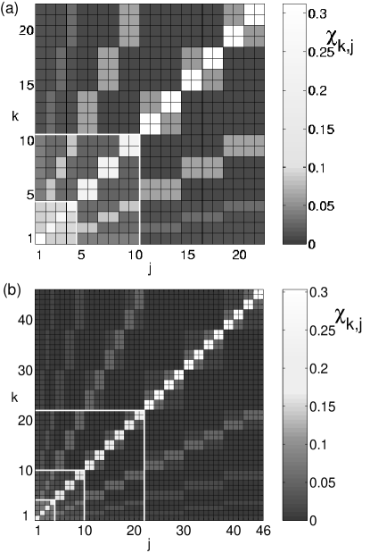
Figure 5: Limiting probabilities for dendrimers with (a) $G=3$ and (b) $G=4$. The white lines indicate the limiting distributions for the dendrimers of generations smaller than $G$.

Figure 5 shows the LPs $\chi_{k,j}$ as a contour plot where the axes are labeled by the nodes $k=1,\cdots,N$ and $j=1,\cdots,N$. Bright shadings correspond to high values of the LP, whereas dark shadings correspond to low LPs. The diagonal has high values, meaning that excitations starting at any node $j$ have a high LP to be at node $j$ again. Note that all values of $\chi_{k,j}$ are clearly larger than the lower bound given in Eq. (13), which is $(1/22)^{2}$ for the $G=3$ dendrimer and $(1/46)^{2}$ for the $G=4$ dendrimer.

The structures of the LP distributions of dendrimers are self-similar generation after generation. The white lines in Fig. 5 are a guide to the eye, indicating this fact.

Furthermore, different nodes $k$ and $l$ may have the same LP, $\chi_{k,j}=\chi_{l,j}$. We hence combine all the nodes having (up to our numerical precision, $10^{-10}$) the same LP into a cluster. Note, however, that the separation of the nodes into clusters depends on the initially excited node, namely on $j$. For an excitation starting at the center (node $1$), the clusters correspond exactly to the different generations of the dendrimer. In the general case, when starting from a non-central node, we still find from Fig. 5 that nodes belonging to the same cluster also belong to the same generation (the converse is not necessarily true).

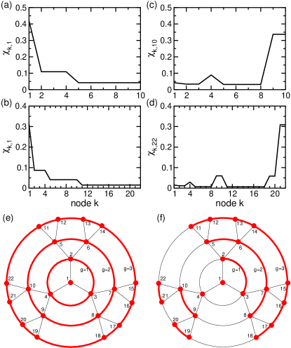
Figure 6: (Color online). Upper two panels: Limiting probabilities for the $G=2$ (top row) and the $G=3$ (bottom row) dendrimer when the excitation starts from the central node $1$ [(a) and (b)] and from one of the outermost nodes [(c) from node $10$ and (d) from node $22$].
Lower panel: Groups of nodes (clusters) having the same limiting probability $\chi_{k,j}$ for a dendrimer of generation $G=3$. In (e) the excitation starts from node $1$ and in (f) from node $22$. Nodes connected by thick (red) lines belong to the same cluster.

We now focus on the two special cases of initial excitations given in the previous sections. Figure 6 presents the LP distributions for the $G=2$ and $G=3$ dendrimers; in both cases the excitation starts either at the central node $1$ or at one of the outermost nodes (node $10$ for $G=2$ and node $22$ for $G=3$).

Having the initial excitation at the central node results in a totally symmetric LP distribution, i.e. in each generation all nodes have the same LP. In this case we can again simplify the problem by considering only the cumulative probabilities. The LP given in Eq. (9) simplifies, because the cumulative probabilities contain only nondegenerate eigenvalues, i.e.

$$\chi_{g,g^{\prime}}=\sum_{n}\left|\langle g|\tilde{q}_{n}\rangle\right|^{2}\left|\langle\tilde{q}_{n}|g^{\prime}\rangle\right|^{2}.$$ (14)

Here, the $|\tilde{q}_{n}\rangle$ are the eigenstates of the reduced Hamiltonian $\tilde{\bf H}$, which does not have degenerate eigenvalues. For the totally recurrent case of an excitation starting at the center of the $G=2$ dendrimer, the LP distribution follows directly from Eq. (2) as

$$\chi_{k,1}=a_{0}^{(k)}.$$ (15)

Note that for an excitation starting at the center the number of different clusters equals $G+1$.

For an excitation starting from one of the outermost nodes, the LPs are less regular. However, also in this case the LPs cluster. Figure 6(f) shows the situation for the $G=3$ dendrimer when starting from node $j=22$. Here, nodes belonging to the same cluster are connected by thick (red) lines. The cluster structure beyond the central node $1$ can be understood on simple symmetry grounds. The structure on the side of the initial node, however, is more complex. Here, nodes $22$ and $21$ have the same LP and form one cluster. The same holds (remarkably) for nodes $9$ and $10$ (another cluster) and for nodes $19$ and $20$ (yet another cluster).

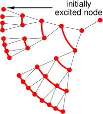
Figure 7: (Color online). Clusters of the same limiting probability $\chi_{k,j}$ in the branch with the initial excitation for a dendrimer of generation $G$. Nodes connected by thick (red) lines belong to the same cluster.

For larger dendrimers, while the general cluster pattern is preserved, some details change. Figure 7 shows the situation for a dendrimer of dimension $G=5$, for an excitation starting at a peripheral node. Again we indicate clusters by connecting nodes by thick (red) lines. A change to be noticed is that for $G\geq 5$ the initially excited node does not form anymore a cluster with its next-nearest node of the same generation. It appears as if such two nodes belong to the same cluster only when the dendrimer has $G\leq 4$. Thus the total number of clusters is $N_{C}\equiv(G^{2}+G+6)/2$ for $G\geq 5$ and $N_{C}-1$ for $G\leq 4$. Moreover, the study of the dendrimer with $G=6$ shows an analogous situation to our findings for $G=5$.

IV.5 Averaged probabilities

One interesting question to ask is, what is the probability, $\pi_{j,j}(t)$, to be at the initial site after some time $t$? As shown above, for the $G=2$ dendrimer $\pi_{k,1}(t)$ and hence $\pi_{1,1}(t)$ are periodic. However, for larger dendrimers and/or different initial conditions this does not have to be the case.

Classically, there exists a simple expression for the average probability to be still or again at the initially excited node. One has (see e.g. Ref. Blumen et al. (2005)):

$$\overline{p}(t)\equiv\frac{1}{N}\sum_{j=1}^{N}p_{j,j}(t)=\frac{1}{N}\sum_{n=1}^{N}\ \exp\big{(}-\lambda_{n}t\big{)}.$$ (16)

This result is quite remarkable, since it depends only on the eigenvalue spectrum of the connectivity matrix ${\bf A}$ but not on the eigenvectors.

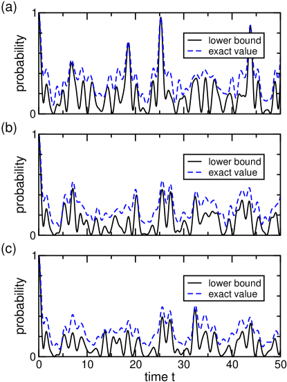
Figure 8: (Color online). Comparison of the averaged probability to be still or again at the initial node with the lower bound given in Eq. (20) for generations (a) $G=2$, (b) $G=3$, and (c) $G=4$.

Quantum mechanically, the average is given by

$$\overline{\pi}(t)\equiv\frac{1}{N}\sum_{j=1}^{N}\pi_{j,j}(t).$$ (17)

By using the Cauchy-Schwarz inequality we obtain a lower bound for $\overline{\pi}(t)$,

$$\overline{\pi}(t)=\frac{1}{N}\sum_{j=1}^{N}|\alpha_{j,j}|^{2}\frac{1}{N}\sum_{l=1}^{N}1\geq\left|\frac{1}{N}\sum_{j}\alpha_{j,j}\right|^{2}.$$ (18)

With Eq. (1) we have

$$\sum_{j}\alpha_{j,j}=\sum_{j}\sum_{n}e^{-it\lambda_{n}}\langle q_{n}|j\rangle\langle j|q_{n}\rangle=\sum_{n}e^{-it\lambda_{n}},$$ (19)

and therefore

$$\overline{\pi}(t)\geq\frac{1}{N^{2}}\sum_{n,m}\ \exp\big{[}-i(\lambda_{n}-\lambda_{m})t\big{]}.$$ (20)

In analogy to the classical case, the lower bound in Eq. (20) depends only on the eigenvalues and not on the eigenvectors of ${\bf A}$. Note that for a CTQW on a simple regular network with periodic boundary conditions the lower bound in Eq. (20) becomes exact.Blumen et al. (2006); Volta et al. (2006)

Figure 8 shows the exact value of the average probability $\overline{\pi}(t)$ as well as the lower bound given in Eq. (20) for dendrimers of three different generations. One notes immediately that the fluctuations of the lower bound are larger that the ones of the exact value. However, the qualitative agreement between the two curves is remarkable: The positions in time of the extrema of the lower bound and of the exact curve almost coincide. Especially the strong maxima of $\overline{\pi}(t)$ are well reproduced by the lower bound.

In fact, fluorescence spectroscopy experiments like, e.g., the ones of Varnavski et al.Varnavski et al. (2002a, b) allow, in principle, to distinguish whether the transport is rather classical or rather quantum mechanical. In order to identify excitonic coherence, Lupton et al. compared a coupled harmonic oscillator model to photoluminescence spectra.Lupton et al. (2002b) Another suggestion is the one by Heijs et al., in which pump-probe and fluorescence experiments determine the efficiency of the excitation transfer,Heijs et al. (2004) from which one can infer the underlying transport mechanism. We close by noting that such models are, as a rule, quite idealized, so that one must be careful in relating the models to the experimental findings.

V Conclusions

In conclusion, we have modelled the coherent exciton transport by continuous-time quantum walks. The transport is exclusively determined by the topology of the dendrimer, i.e. by its connectivity matrix. For the $G=2$ dendrimer the transport is completely recurrent when the central node is initially excited. In this case the quantum mechanical transition probabilities are fully periodic. For larger dendrimers and/or different initial conditions we observe only partial recurrences.

To compare these results to those of the classical (incoherent) case, we calculated the long time average of the transition probabilities. Depending on the initial conditions, these show characteristic patterns. Furthermore, the limiting probability distributions can be characterized by clusters of nodes having the same limiting probabilities.

Furthermore, we calculated a lower bound for the average probability to be still or again at the initial node after some time $t$. This lower bound depends only on the eigenvalues of ${\bf A}$ and agrees qualitatively well with the exact value; especially the maxima of $\overline{\pi}(t)$ are well reproduced by the lower bound.

References

- Vögtle (1998) F. Vögtle, ed., Dendrimers (Springer, Berlin, 1998).
- jlu (2005) J. Lumin. 111, Issue 4 (2005).
- Mukamel (1997) S. Mukamel, Nature 388, 425 (1997).
- Jiang and Aida (1997) D.-J. Jiang and T. Aida, Nature 388, 454 (1997).
- Bar-Haim and Klafter (1998) A. Bar-Haim and J. Klafter, J. Lumin. 76&77, 197 (1998).
- Flomenbom et al. (2005) O. Flomenbom, R. J. Amir, D. Shabat, and J. Klafter, J. Lumin. 111, 315 (2005).
- Kopelman et al. (1997) R. Kopelman, M. Shortreed, Z.-Y. Shi, W. Tan, Z. Xu, J. S. Moore, A. Bar-Haim, and J. Klafter, Phys. Rev. Lett. 78, 1239 (1997).
- Shortreed et al. (1997) M. R. Shortreed, S. F. Swallen, Z.-Y. Shi, W. Tan, Z. Xu, C. Devadoss, J. S. Moore, and R. Kopelman, J. Phys. Chem. B 101, 6318 (1997).
- Lupton et al. (2001) J. M. Lupton, R. Beavington, P. L. Burn, I. D. W. Samuel, and H. Bässler, Synth. Met. 121, 1703 (2001).
- Varnavski et al. (2002a) O. Varnavski, I. D. W. Samuel, L.-O. P lsson, R. Beavington, P. L. Burn, and T. G. III, J. Chem. Phys. 116, 8893 (2002a).
- Varnavski et al. (2002b) O. P. Varnavski, J. C. Ostrowski, L. Sukhomlinova, R. J. Twieg, G. C. Bazan, and T. G. III, J. Am. Chem. Soc. 124, 1736 (2002b).
- Bharathi et al. (1995) P. Bharathi, U. Patel, T. Kawaguchi, D. J. Pesak, and J. S. Moore, Macromolecules 28, 5955 (1995).
- Poliakov et al. (1999) E. Y. Poliakov, V. Chernyak, S. Tretiak, and S. Mukamel, J. Chem. Phys. 110, 8161 (1999).
- Kenkre and Reineker (1982) V. M. Kenkre and P. Reineker, Exciton Dynamics in Molecular Crystals and Aggregates (Springer, Berlin, 1982).
- Shore (1990) B. W. Shore, The Theory of Coherent Atomic Excitation (Wiley, New York, 1990).
- Davydov (1962) A. S. Davydov, Theory of Molecular Excitons (McGraw-Hill, New York, 1962).
- Haken (1976) H. Haken, Quantum Field Theory of Solids (North-Holland, Amsterdam, 1976).
- Heijs et al. (2004) D.-J. Heijs, V. A. Malyshev, and J. Knoester, J. Chem. Phys. 121, 4884 (2004).
- Vlaming et al. (2005) S. M. Vlaming, D. J. Heijs, and J. Knoester, J. Lumin. 111, 349 (2005).
- Blumen et al. (2005) A. Blumen, A. Volta, A. Jurjiu, and T. Koslowski, J. Lumin. 111, 327 (2005).
- Mülken and Blumen (2005a) O. Mülken and A. Blumen, Phys. Rev. E 71, 016101 (2005a).
- Mülken and Blumen (2005b) O. Mülken and A. Blumen, Phys. Rev. E 71, 036128 (2005b).
- Mülken et al. (2005) O. Mülken, A. Volta, and A. Blumen, Phys. Rev. A 72, 042334 (2005).
- Mülken and Blumen (2006) O. Mülken and A. Blumen, Phys. Rev. A (2006), in press.
- McQuarrie (1983) D. A. McQuarrie, Quantum Chemistry (Oxford University Press, Oxford, 1983).
- Weiss (1994) G. H. Weiss, Aspects and Applications of the Random Walk (North-Holland, Amsterdam, 1994).
- van Kampen (1990) N. van Kampen, Stochastic Processes in Physics and Chemistry (North-Holland, Amsterdam, 1990).
- Farhi and Gutmann (1998) E. Farhi and S. Gutmann, Phys. Rev. A 58, 915 (1998).
- Childs et al. (2002) A. M. Childs, E. Farhi, and S. Gutmann, Quantum Information Processing 1, 35 (2002).
- Cai and Chen (1997) C. Cai and Z. Y. Chen, Macromolecules 30, 5104 (1997).
- Kinzel (1995) W. Kinzel, Phys. Bl. 51, 1190 (1995).
- Grossmann et al. (1997) F. Grossmann, J.-M. Rost, and W. P. Schleich, J. Phys. A 30, L277 (1997).
- Iwanow et al. (2005) R. Iwanow, D. A. May-Arrioja, D. N. Christodoulides, G. I. Stegeman, Y. Min, and W. Sohler, Phys. Rev. Lett. 95, 053902 (2005).
- Bar-Haim et al. (1997) A. Bar-Haim, J. Klafter, and R. Kopelman, J. Am. Chem. Soc. 119, 6197 (1997).
- Rana and Gangopadhyay (2003) D. Rana and G. Gangopadhyay, J. Chem. Phys. 118, 434 (2003).
- Aharonov et al. (2001) D. Aharonov, A. Ambainis, J. Kempe, and U. Vazirani, in Proceedings of ACM Symposium on Theory of Computation (STOC’01) (ACM Press, New York, 2001), p. 50.
- Abramowitz and Stegun (1972) M. Abramowitz and I. A. Stegun, eds., Handbook of Mathematical Functions (Dover, New York, 1972).
- Blumen et al. (2006) A. Blumen, V. Bierbaum, and O. Mülken, Physica A (2006), submitted.
- Volta et al. (2006) A. Volta, O. Mülken, and A. Blumen (2006), in preparation.
- Lupton et al. (2002b) J. M. Lupton, I. D. W. Samuel, P. L. Burn, and S. Mukamel, J. Phys. Chem. B 106, 7647 (2002b).