Two-dimensional Heisenberg antiferromagnet in a transverse field

Abstract

We investigate the magnetic reorientation in a two-dimensional anisotropic antiferromagnet due to a transverse magnetic field. Using a many-body Green’s function approach, we show that the magnetization component perpendicular to the applied field (and along the easy-axis of the antiferromagnet) initially increases with increasing field strength. We show that this unexpected result arises from the suppression of quantum and thermal fluctuations in the antiferromagnet. Above the Néel temperature, this effect leads to a reappearance of a magnetic moment along the easy-axis.

I Introduction

The magnetic properties of two-dimensional (2D) antiferromagnets (AFM) have been extensively studied in the past. TaI91 ; IKK99 ; CRT03 ; ZhN98 ; ZhC99 ; PMB99 Examples of 2D AFMs that have been recently investigated include the manganites which exhibit a colossal magnetoresistance,JTC94 the vanadates,MAT01 and the undoped parent compounds of the high-temperature superconductors.BGJ88 The latter are a prime example of weakly anisotropic 2D AFMs due to their small in-plane anisotropy and an even smaller interlayer coupling between neighboring CuO₂-planes. A finite anisotropy is necessary to stabilize the long-range magnetic order in 2D magnets at finite temperatures.MeW66 Even a rather weak anisotropy induces an ordering temperature of the same magnitude as the isotropic exchange. Lin64 The properties of the above materials have been intensely studied theoretically within the framework of the Heisenberg model. TaI91 ; IKK99 ; CRT03 ; BGJ88 ; DmK04 ; HSL05 ; BBG98 ; Din90 In particular, the magnetization of the isotropic 2D AFM as function of an applied magnetic field have been studied within spin-wave theory.ZhN98 ; ZhC99 ; PMB99

In this communication we study the properties of a 2D anisotropic AFM with spin $S=1/2$ on a square lattice in a transverse magnetic field perpendicular to the easy axis of the anisotropy. To this end, we develop a many-body Green’s function method Tya67 that is based on the equation-of-motion formalism. Our results are two-fold. First, the staggered AFM magnetization along the easy axis increases with increasing strength of the transverse magnetic field. This effect is quite unexpected since the field is directed perpendicular to the magnetization component. We find, however, that the presence of a weak transverse field leads to the suppression of quantum and thermal fluctuations in the AFM, the former being responsible for the decrease of the zero temperature sublattice magnetization from its saturation value, $S=1/2$. While a similar behavior has been predicted for one-dimensional (1D) AFM spin chains,DmK04 its relation to our results is at present unclear due to the qualitatively different nature of spin excitations in 1D and 2D systems. Second, the AFM ordered spins take a noncollinear canted orientation for any non-zero transverse field, inducing a non-zero magnetization component parallel to the applied field. Note that this behavior is qualitatively different from that of a 2D AFM in a longitudinal magnetic field parallel to the easy axis.CRT03 ; HSL05 In the latter, a canted spin configuration can only be reached via a phase transition into the so-called spin-flop-phase.

II Theory

We consider the anisotropic (XXZ-) Heisenberg Hamiltonian

$$\mathcal{H}=\frac{1}{2}\sum_{\mathord{\langle}ij\mathord{\rangle}}\,\Big{[}J\;\mathbf{S}_{i}\,\mathbf{S}_{j}+D\,S_{i}^{z}\,S_{j}^{z}\Big{]}-B_{x}\,\sum_{i}\,S_{i}^{x}\,,$$ (1)

where $\mathbf{S}_{i}$ is the spin operator with spin quantum number $S=1/2$ located on sites $i$ of a square lattice, and $J>0$ is the isotropic exchange coupling between nearest neighbor (nn) spin pairs $i$ and $j$. The easy-axis is modeled by an exchange anisotropy $D>0$ along the $z$-axis. We take the transverse magnetic field $\mathbf{B}=(B_{x},0,0)$ to be aligned along the $x$-axis, perpendicular to the easy axis. Similar results to the ones discussed below are expected for a single-ion anisotropy, although its physical origin differs from the exchange anisotropy considered in this study.FrK03

In order to compute the temperature- and field-dependence of the AFM’s sublattice magnetization $\mathbf{m}_{i}(T,B_{x})$, we employ a many-body Green’s function approach, which is based on the equation-of-motion formalism.Tya67 The non-collinear magnetic structure which occurs in the presence of a non-zero transverse magnetic field requires that two non-vanishing magnetization components have to be considered. This can be done either in the original spin coordinate system,FJK00 which however is analytically and numerically demanding due to the occurring zero-eigenvalue problem.FrK05 Therefore, we apply an approach identical to the one recently used to investigate the field-induced spin reorientation of 2D anisotropic ferromagnets, SKN05 ; PPS05 and to study the noncolllinear magnetization of 2D isotropic antiferromagnets.ZhN98 ; ZhC99 ; PMB99 In this approach, the spins of each sublattice $i$ are rotated locally by angles $\theta_{i}$ in such a way that in the rotated frame (primed spin operators) only a single non-vanishing component of the sublattice magnetization remains, i.e., $m_{i}(T)=\mathord{\langle}{S_{i}^{z}}^{\prime}\mathord{\rangle}\neq 0$ and $\mathord{\langle}{S_{i}^{x}}^{\prime}\mathord{\rangle}=\mathord{\langle}{S_{i}^{y}}^{\prime}\mathord{\rangle}=0$. The symmetry of the present case simplifies the calculation considerably by assuming equal magnitudes of the sublattice magnetization, $m(T,B_{x})=|{\bf m}_{1}(T,B_{x})|=|{\bf m}_{2}(T,B_{x})|$, and canting angles $\theta_{1}(T)=\theta(T)$ and $\theta_{2}(T)=\pi-\theta(T)$ with respect to the easy axis.

Specifically, we consider the following commutator Green’s functions in energy space,

$$G_{ij}^{\pm}(\omega)=\mathord{\langle}\mathord{\langle}{S_{i}^{\pm}}^{\prime};{S_{j}^{-}}^{\prime}\mathord{\rangle}\mathord{\rangle}_{\omega}\,,$$ (2)

which we compute by the conventional equation-of-motion approach. We approximate higher-order Green’s functions by using the Tyablikov decoupling for $i\neq k$,Tya59

$$\mathord{\langle}\mathord{\langle}{S_{i}^{z}}^{\prime}\,{S_{k}^{\pm}}^{\prime};{S_{j}^{-}}^{\prime}\mathord{\rangle}\mathord{\rangle}_{\omega}\sim\mathord{\langle}{S_{i}^{z}}^{\prime}\mathord{\rangle}\mathord{\langle}\mathord{\langle}{S_{k}^{\pm}}^{\prime};{S_{j}^{-}}^{\prime}\mathord{\rangle}\mathord{\rangle}_{\omega}=m_{i}(T)\;G_{kj}^{\pm}(\omega)\;.$$ (3)

For 2D ferromagnets with a small anisotropy it has been shown that the Tyablikov decoupling (or random-phase approximation, RPA) yields almost quantitative results specifically for the magnetization and susceptibilities,HFK02 whereas the resulting free energy and the specific heat are less well described.JIR04 For systems with spin quantum number $S=1/2$ the magnetization can now be obtained from

$$m(T)=1/2-\frac{1}{N}\;\sum_{\mathbf{k}}\mathord{\langle}{S_{1}^{-}}^{\prime}{S_{1}^{+}}^{\prime}\mathord{\rangle}(\mathbf{k})\;,$$ (4)

where $N$ is the number of lattice sites, and the momentum sum runs over the full Brillouin zone. The equal-time correlation function $\mathord{\langle}{S_{1}^{-}}^{\prime}{S_{1}^{+}}^{\prime}\mathord{\rangle}(\mathbf{k})$ is obtained after Fourier transformation into momentum space from Eq.(2) via the spectral theorem.Tya67 Note that here the indices $i,j=1,2$ refer to the two sublattices. We obtain

$$\mathord{\langle}{S_{1}^{-}}^{\prime}\,{S_{1}^{+}}^{\prime}\mathord{\rangle}(\mathbf{k}) = \frac{m(T)}{2}\;\bigg{[}\frac{a+b(\mathbf{k})}{\varepsilon_{1}(\mathbf{k})}\;\coth\bigg{(}\frac{\beta\varepsilon_{1}(\mathbf{k})}{2}\bigg{)}$$ (5)

$$+\frac{a-b(\mathbf{k})}{\varepsilon_{2}(\mathbf{k})}\;\coth\bigg{(}\frac{\beta\varepsilon_{2}(\mathbf{k})}{2}\bigg{)}-2\bigg{]}\;,$$

where

$$a = B_{x}\,\sin\theta(T)$$ (6)

$$+ \!\!q\,m(T)\,\big{[}J+D-(2\,J+D)\,\sin^{2}\theta(T)\big{]}\,,$$

$$b(\mathbf{k}) = -m(T)\,\gamma(\mathbf{k})\,(J+D/2)\,\sin^{2}\theta(T)\,,$$ (7)

$$c(\mathbf{k}) = m(T)\,\gamma(\mathbf{k})\,\big{[}J-(J+D/2)\,\sin^{2}\theta(T)\big{]}\,,$$ (8)

$$\varepsilon_{1,2}^{2}(\mathbf{k}) = [a\pm b(\mathbf{k})]^{2}-c^{2}(\mathbf{k})\,.$$ (9)

$$\gamma(\mathbf{k}) = 2\,(\cos k_{x}+\cos k_{y})\,.$$ (10)

Here, $q=4$ is the number of nearest neighbor sites, and the lattice constant $a_{0}$ is set to unity. The excitations of the system are represented by two branches of spin waves whose dispersions are given by $\varepsilon_{1,2}(\mathbf{k})$. For $\mathbf{B}=0,\theta=0$ the Néel temperature $T_{N}$ is given by

$$T_{N} = \frac{1}{4}\;\left(\frac{1}{N}\,\sum_{\mathbf{k}}\frac{\overline{a}}{\overline{a}^{2}-(J\gamma(\mathbf{k}))^{2}}\right)^{-1}$$ (11)

$$\approx \pi\,J\Big{/}\ln\Big{(}\frac{J\,\pi^{2}}{q\,D}\Big{)}\;,$$

with $\overline{a}=q\,(J+D)$. Note that the “anomalous” Green’s function $G_{ij}^{-}(\omega)$ appears due to the canted nature of the spin configuration in a transverse field. Its appearance implies that in addition to the spin-flip term ${S^{-}}^{\prime}{S^{+}}^{\prime}$ also a term of the form ${S^{-}}^{\prime}{S^{-}}^{\prime}$ is present in the Hamiltonian.TaI91 ; Mil89 As a consequence, the spin precession around the equilibrium direction is no longer spherical but elliptical. Also, the consideration of $G_{ij}^{-}(\omega)$ guarantees that the Mermin-Wagner theorem is fulfilled for an easy-plane magnet ($D<0$).

In order to obtain the individual components of the magnetization, we need to compute the magnetization angle $\theta_{0}(T,B_{x})$. free The latter can be obtained from the observation that in the rotated frame in equilibrium no torque is exerted on the magnetization $\mathord{\langle}{S_{i}^{z}}^{\prime}\mathord{\rangle}$, i.e., ${S_{i}^{z}}^{\prime}$ is a constant of the motion, and $d\mathord{\langle}{S_{i}^{z}}^{\prime}\mathord{\rangle}/dt=0$. This requirement, in turn, is equivalent to the condition that the Green’s function $G_{ij}^{z}(\omega)=\mathord{\langle}\mathord{\langle}{S_{i}^{z}}^{\prime};{S_{j}^{-}}^{\prime}\mathord{\rangle}\mathord{\rangle}_{\omega}$ vanishes, as has been shown for the field-induced spin reorientation of a ferromagnetic monolayer.PPS05 Computing this Green’s function by using the same treatment as for the $G_{ij}^{\pm}(\omega)$- Green’s functions, i.e., by application of the Tyablikov decoupling, one finds

$$\hskip 28.45274pt\sin\theta_{0}(T,B_{x})=$$ (12)

$$\begin{cases}\frac{\displaystyle B_{x}}{\displaystyle q\,m(T,B_{x})\,(2J+D)}\;,\quad&B_{x}<q\,m(T,B_{x})\,(2J+D)\;,\\ \hskip 42.67912pt1\;,&\hskip 28.45274pt\mathrm{otherwise}\;.\end{cases}$$

This method to determine the angle $\theta_{0}(T,B_{x})$ was successfully applied by Schwieger et al. SKN05 and by Pini et al. PPS05  for the case of the field-induced spin reorientation of a 2D ferromagnet.

For $T=0$ we have compared this approach with the one where $\theta_{0}(0,B_{x})$ is determined from the minimum of the internal energy $E(0,\theta)=\mathord{\langle}\mathcal{H}\mathord{\rangle}$, and found satisfactory agreement. In fact, the relation Eq.(12) for $\theta_{0}(T,B_{x})$ is identical to the one calculated from the free energy $F_{\mathrm{MFA}}(T,\theta)$ within a single-site mean field approximation. This approximation is easily obtained within our theoretical approach by neglecting the spin-flip term $S_{i}^{+}S_{j}^{-}$ in Eq.(1), or putting $\gamma(\mathbf{k})=0$ in Eqs.(7)-(9).free

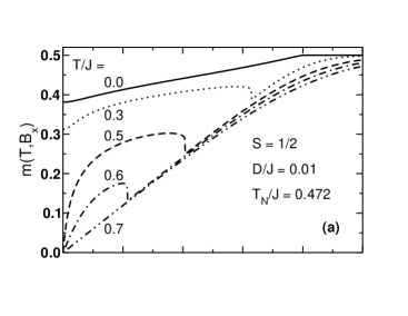
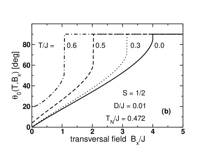
Figure 1: (a) Magnetization $m(T,B_{x})$ and (b) equilibrium angle $\theta_{0}(T,B_{x})$ as functions of the transversal field $B_{x}$ for different temperatures $T$ below and above the Néel temperature $T_{N}$. The temperatures and interactions are given in units of the isotropic exchange $J$. We have assumed a spin quantum number $S=1/2$ and an anisotropy $D/J=0.01$.

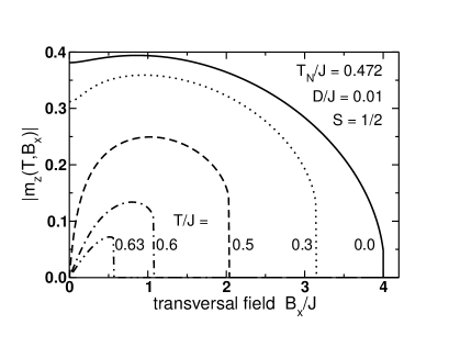
Figure 2: Staggered magnetization component $|m_{z}(T,B_{x})|$ along the easy axis as function of the transversal field $B_{x}$ for different temperatures $T$. For the other denotations we refer to Fig. 1.

III Results

Unless stated otherwise, we consider in the following a weak anisotropy $D/J=0.01$, yielding a sublattice magnetization of $m(T=0,B_{x}=0)=0.381$ at $T=0$. A magnetic anisotropy is necessary since for an isotropic system (i.e., for $D=B_{x}=0$), our approach satisfies the Mermin-Wagner-theorem MeW66 ; Tya67 and we have $m\equiv 0$ at $T\not=0$. For the isotropic 2D AFM ($D=0$) on a square lattice we obtain $m(T=0,B_{x}=0)\sim 0.36$, which compares reasonably well with the commonly accepted value of $0.307$. BBG98 The latter value is also obtained within the Holstein-Primakoff-approximation. The Néel temperature $T_{N}$ for $D/J=0.01$ is calculated to be $T_{N}/J=0.472$, while a quantum Monte Carlo calculation yields a larger transition temperature of $T_{N}/J=0.590$ for the same system.Din90 In Fig. 1 we present the magnitude of the magnetization, $m(T,B_{x})$, and the equilibrium angle, $\theta_{0}(T,B_{x})$, as a function of the transverse field $B_{x}$ for temperatures $T$ below and above $T_{N}$. For all temperatures, the magnetization $m(T,B_{x})$ increases when $B_{x}$ is increased from zero. At the same time, $\theta_{0}(T,B_{x})$ also increases with increasing $B_{x}$, indicating that the magnetization is rotated towards the direction of the transverse field. Moreover, for $T<T_{N}$, the angle $\theta_{0}(T,B_{x})$ deviates from zero for infinitesimally small $B_{x}$, implying that the rotation of the staggered moment does not require a critical field strength, in contrast to the spin-flop transition associated with the application of a longitudinal magnetic field.CRT03 ; HSL05 Note that for $T>T_{N}$, the limit $B_{x}\to 0$ leads to a non-zero angle $\theta_{0}(T,B_{x})<\pi/2$. This implies that a non-zero $|m_{z}(T,B_{x})|$ is induced by the transverse field, and that the component of the induced magnetization parallel to the transverse field increases faster than the component parallel to the easy axis. For $T/J>0.64$ the behavior corresponds to the magnetization of an isotropic AFM.ZhN98

The reorientation field $B_{R}(T)=4m(T,B_{R})(2J+D)$ is the smallest field at which the magnetization is parallel to the direction of the magnetic field, i.e., $\theta_{0}(T,B_{R})=\pi/2$. Both $m(T,B_{x})$ and $\theta_{0}(T,B_{x})$ exhibit a discontinuous behavior at the reorientation field. Specifically, $m(T,B_{x})$ jumps at $B_{R}(T)$ to a smaller value and increases with further increasing $B_{x}>B_{R}(T)$. At the same time, the angle $\theta_{0}(T,B_{x})$ jumps from $\theta<\pi/2$ to $\pi/2$ at $B_{R}$. Presently we cannot judge whether this discontinuous behavior is ‘real’ or an artefact of the approximations used above.

The staggered magnetization component $|m_{z}(T,B_{x})|$ along the easy ($z$-) axis as computed from $m(T,B_{x})$ and $\theta_{0}(T,B_{x})$ is shown in Fig. 2 as function of $B_{x}$. Though this magnetization component is perpendicular to the applied field, we find that it also increases when $B_{x}$ is increased from zero. This behavior is quite unexpected since the rotation of $\mathbf{m}(T,B_{x})$ into the direction of the transverse field should lead to a decrease in $|m_{z}(T,B_{x})|$. After passing through a maximum, $|m_{z}(T,B_{x})|$ discontinuously vanishes at the reorientation field $B_{R}(T)$. At the same time, the magnetization component $m_{x}(T,B_{x})$ along the magnetic field increases linearly with $B_{x}$, and saturates for $B_{x}>B_{R}(T)$. As mentioned, for $T>T_{N}$ a non-zero $B_{x}$ induces a finite $|m_{z}(T,B_{x})|$ which increases continuously from $|m_{z}|=0$ in the disordered (paramagnetic) state for $B_{x}=0$, exhibits a maximum, and then vanishes at the reorientation field. Moreover, in the limit $J=0$, i.e., for a purely ‘Ising’-like exchange $D$ where the transversal magnetization components are missing, we obtain that $|m_{z}(T,B_{x})|$ does not exhibit a maximum, but decreases monotonically.

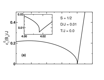
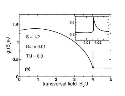
Figure 3: (a) Energy gap $\varepsilon_{1}^{0}(B_{x})$ and (b) spinwave stiffness $g_{1}(B_{x})$, cf. Eqs.(12,14), of the magnon dispersion relation $\varepsilon_{1}(B_{x})$ as function of the transversal field $B_{x}$ for $T=0$. The insets show the behaviors of $\varepsilon_{1}^{0}(B_{x})$ and $g_{1}(B_{x})$ near the reorientation field $B_{R}(0)/J\sim 4.0162$. For the other denotations we refer to Fig. 1.

The increase of $|m_{z}|$ for small $B_{x}$ can be attributed to the suppression of quantum and thermal fluctuations, whose strength depends on the form of the magnon excitations spectrum. At $T=0$, quantum fluctuations lead to a reduction of the staggered magnetization $|m_{z}|$ from its saturation value given by $S=1/2$. In order to investigate the strength of quantum fluctuations, we consider the magnon dispersion, $\varepsilon_{1,2}(\mathbf{k})$ as a function of the transverse field $B_{x}$ at $T=0$. Near the center of the Brillouin zone at ${\bf k}=0$ we expand the dispersion to obtain

$$\varepsilon_{1,2}(\mathbf{k})=\varepsilon_{1,2}^{0}(B_{x})+g_{1,2}(B_{x})\,\mathbf{k}^{2}\;,$$ (13)

where $\varepsilon_{1,2}^{0}$ is the energy gap (‘mass’) and $g_{1,2}$ the spinwave stiffness of the dispersion. For fields smaller than the reorientation field $B_{R}(0)$, we find

$$\varepsilon_{1}^{0}(B_{x}) = \sqrt{\frac{D}{2J+D}\;\Big{[}(4m)^{2}\,(2J+D)^{2}-B_{x}^{2}\Big{]}}\;,$$ (14)

$$\varepsilon_{2}^{0}(B_{x}) = \sqrt{(4m)^{2}\,D\,(2J+D)+B_{x}^{2}}\;.$$ (15)

In Fig. 3 we present $\varepsilon_{1}^{0}(B_{x})$ and $g_{1}(B_{x})$ for the lower-energy magnon branch. Both quantities increase as $B_{x}$ is increased from zero and exhibit a maximum at $B_{x}/J\sim 0.85$ which coincides with the location of the maximum in $|m_{z}|$. The increase of the excitation gap and of the spin stiffness reduce the strength of fluctuations, and are thus directly responsible for the increase in $|m_{z}|$. A decreasing anisotropy $D/J$ yields a smaller gap, which increases the strength of the fluctuations, and as a result, the maximum of $|m_{z}(0,B_{x})|$ becomes more pronounced. For $B_{x}\to B_{R}(0)$ the dispersion softens,PPS05 however, the gap retains a small but still finite value at the reorientation field $B_{R}(0)$. At the same time $g_{1}(B_{x})$ exhibits a pronounced spike. These features are responsible for the discontinuous behavior of the magnetization at the reorientation field discussed above. Note that for $T>T_{N}$ and for a finite $B_{x}$ the dispersions $\varepsilon_{1,2}(T,B_{x})$ do not become ‘soft’ but exhibit as expected a gap even when the magnetization is completely aligned with the transverse field, i.e., for $\theta_{0}(T,B_{x})=\pi/2$.

The increase of $|m_{z}(T,B_{x})|$ at small $B_{x}$ is pronounced for systems where quantum fluctuations are most important, i.e., for a small spin quantum number $S$ and for a low spatial dimensionality. Our calculations show that with increasing $S$ the relative maximum of $|m_{z}(T,B_{x})|$ becomes smaller, and is not present at all for $S=\infty$, i.e., for classical spins.

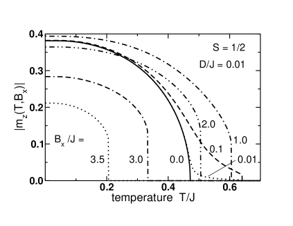
Figure 4: Staggered magnetization component $|m_{z}(T,B_{x})|$ along the easy axis as function of the temperature for different $B_{x}$. For the other denotations we refer to Fig. 1.

In Fig. 4, we plot $|m_{z}(T,B_{x})|$ as a function of the temperature for various magnetic fields. We define the temperature at which $|m_{z}|$ vanishes as the reorientation temperature $T_{R}(B_{x})$, with $T_{R}(B_{x}=0)=T_{N}$. Note that already a weak magnetic field leads to a $T_{R}$ that is significantly larger than $T_{N}$. With further increasing $B_{x}$ the reorientation temperature decreases and vanishes for $B_{x}/J>4.02$.

In the remainder of this Section we will briefly mention related results that were obtained in other systems and by using different theoretical approaches. A maximum of $|m_{z}(T,B_{x})|$ has recently been obtained for an anisotropic AFM Heisenberg chain.DmK04 Here $|m_{z}(T,B_{x})|$ increases from the paramagnetic state $|m_{z}|=0$, since such a chain does not exhibit an ordered state, and corresponds thus to temperatures $T>T_{N}$ for the 2D AFM as investigated in this study. Solving the latter system with a single-spin mean-field approximation, no maximum of $|m_{z}(T,B_{x})|$ is obtained, since the transversal spin terms $S_{i}^{x}\,S_{j}^{x}+S_{i}^{y}\,S_{j}^{y}$ of Eq.(1), which cause the obtained behavior, are neglected by this method. Nevertheless, if these terms are taken into account to some extent, such as within a two-spin mean-field approximation (Oguchi theory Ogu55 ), the properties of $|m_{z}(T,B_{x})|$ are qualitatively reproduced. Finally, a maximum of $|m_{z}(T,|B_{z}|,B_{x})|$ is also obtained for an antiferromagnetically coupled Heisenberg spin pair, a system which can be solved exactly. In this case, for $B_{x}=0$ a finite magnetic order is induced by a small staggered magnetic field $|B_{z}|$ along the $z$-axis.

IV Conclusion

We have studied the magnetization of a 2D square-lattice anisotropic (XXZ-) AFM in a transverse magnetic field. A many-body Green’s function approach has been applied, which is known to yield a good description of the magnetization for the case of a ferromagnetic monolayer.JIR04 The fact that our theoretical approach yields values for the sublattice magnetization at $\mathbf{B}=0$ and the Néel temperature that are similar to those obtained in quantum Monte Carlo calculations Din90 supports the validity of the theoretical method also for the 2D AFM.

We showed that the staggered magnetization $|m_{z}(T,B_{x})|$ along the easy-axis perpendicular to the field increases for small $B_{x}$ and exhibits a maximum before vanishing at the reorientation field. For $T>T_{N}$, we demonstrate that the transverse field induces a non-zero magnetization $|m_{z}(T,B_{x})|$ which is perpendicular to the applied field. We argue that the increase of $|m_{z}(T,B_{x})|$ for small $B_{x}$ arises from changes in the magnon excitation spectrum, which in turn leads to a suppression of thermal and quantum fluctuations.

The described behavior of the staggered magnetization of a 2D AFM in a transverse field can possibly be observed by, e.g., x-ray magnetic linear dichroism (XMLD), since this method is sensitive to the magnitude of the magnetization components.Laa98 An interesting question is whether a finite magnetization component along the easy-axis for temperatures slightly above $T_{N}$ as induced by a transverse magnetic field can be measured, cf. Figs. 2,4.

Note that typical magnetic fields of a few Teslas yield Zeeman energies much smaller than the exchange, $B_{x}\ll J$. Hence, when such a transverse field is applied to the AFM, the canting angle will be small. In contrast, if the AFM is coupled to an ordered ferromagnet (FM), the intrinsic field due to the strong interlayer exchange coupling at the AFM/FM interface is considerably larger. The resulting angle $\theta_{0}(T,B_{x})$ could then be sufficiently large such that the results presented above are observable. A particular interest in such FM – AFM interfaces has revived lately in relation to the exchange bias effect.NoS99

Useful discussions with K. D. Schotte are gratefully acknowledged. P. J. J. likes to thank the IPCMS in Strasbourg, France, for the hospitality, and the Deutsche Forschungsgemeinschaft, Sfb 290, for financial support. D.K.M acknowledges financial support from the Alexander von Humboldt Foundation.

References

- (1) T. Tamaribuchi and M. Ishikawa, Phys. Rev. B 43, R1283 (1991).
- (2) V. Yu. Irkhin, A. A. Katanin, and M. I. Katsnelson, Phys. Rev. B 60, 1082 (1999).
- (3) A. Cuccoli, T. Roscilde, V. Tognetti, R. Vaia, and P. Verrucchi, Phys. Rev. B 67, 104414 (2003).
- (4) M. E. Zhitomirsky and T. Nikuni, Phys. Rev. B 57, 5013 (1998).
- (5) M. E. Zhitomirsky and A.L. Chernyshev, Phys. Rev. Lett. 82, 4536 (1999).
- (6) D. Petitgrand, S. V. Maleyev, Ph. Bourges, and A.S. Ivanov, Phys. Rev. B 59, 1079 (1999); A. V. Syromyatnikov and S. V. Maleyev, Phys. Rev. B 65, 012401 (2002).
- (7) S. Jin, T. H. Tiefel, M. McCormack, R. A. Fastnacht, R. Ramesh, and L. H. Chen, Science 264, 413 (1994).
- (8) R. Melzi, S. Aldrovandi, F. Tedoldi, P. Carretta, P. Millet, and F. Mila, Phys. Rev. B 64, 024409 (2001).
- (9) R. J. Birgeneau et al., Phys. Rev. B 38, 6614 (1988); E. Manousakis, Rev. Mod. Phys. 63, 1 (1991).
- (10) N. D. Mermin and H. Wagner, Phys. Rev. Lett. 17, 1133 (1966).
- (11) M. E. Lines, Phys. Rev. 133, A841 (1964); M. Bander and D. L. Mills, Phys. Rev. B 38, R12015 (1988); R. P. Erickson and D. L. Mills, Phys. Rev. B 43, R11527 (1991).
- (12) D. V. Dmitriev and V. Ya. Krivnov, Phys. Rev. B 70, 144414 (2004).
- (13) M. Holtschneider, W. Selke, and R. Leidl, Phys. Rev. B 72, 064443 (2005).
- (14) B. B. Beard, R. J. Birgeneau, M. Greven, and U. J. Wiese, Phys. Rev. Lett. 80, 1742 (1998); J. K. Kim and M. Troyer, Phys. Rev. Lett. 80, 2705 (1998).
- (15) H. Q. Ding, J. Phys.: Condens. Matter 2, 7979 (1990); S. S. Aplesnin, Phys. Stat. Sol. B 207, 491 (1998).
- (16) S. V. Tyablikov, Methods in the quantum theory of magnetism, Plenum Press, New York, 1967; W. Nolting, Quantentheorie des Magnetismus, vol.2, B. G. Teubner, Stuttgart, 1986.
- (17) P. Fröbrich and P. J. Kuntz, Europ. Phys. J. B 32, 445 (2003).
- (18) P. Fröbrich, P. J. Jensen, and P. J. Kuntz, Europ. Phys. J. B 13, 477 (2000); P. Fröbrich, P. J. Jensen, P. J. Kuntz, and A. Ecker, Europ. Phys. J. B 18, 579 (2000).
- (19) P. Fröbrich and P. J. Kuntz, J. Phys.: Condens. Matter 17, 1167 (2005).
- (20) S. Schwieger, J. Kienert, and W. Nolting, Phys. Rev. B 71, 024428 (2005).
- (21) M. G. Pini, P. Politi, R. L. Stamps, Phys. Rev. B 72, 014454 (2005).
- (22) S. V. Tyablikov, Ukr. Mat. Zh. 11, 287 (1959).
- (23) P. Henelius, P. Fröbrich, P. J. Kuntz, C. Timm, and P. J. Jensen, Phys. Rev. B 66, 094407 (2002).
- (24) I. Junger, D. Ihle, J. Richter, and A. Klümper, Phys. Rev. B 70, 104419 (2004).
- (25) D. L. Mills, Phys. Rev. B 40, 11153 (1989).
- (26) Usually the equilibrium angle should be determined by minimizing the free energy as obtained by the Green’s function approach. Unfortunately, since within the Tyablikov decoupling behaves unphysically at elevated temperatures,JIR04 this approach cannot be applied here.
- (27) T. Oguchi, Progr. Theor. Phys. 13, 148 (1955).
- (28) G. van der Laan, Phys. Rev. B 57, 5250 (1998); J. Lüning, F. Nolting, A. Scholl, H. Ohldag, J. W. Seo, J. Fompeyrine, J.-P. Locquet, and J. Stöhr, Phys. Rev. B 67, 214433 (2003).
- (29) For recent reviews see, e.g.: J. Nogués and I. K. Schuller, J. Magn. Magn. Mater. 192, 203 (1999); M. Kiwi, ibid. 234/3, 584 (2001); R. L. Stamps, J. Phys. D: Appl. Phys. 33, R247 (2000).