Screening in the two-dimensional electron gas with spin-orbit coupling

Abstract

We study screening properties of the two-dimensional electron gas with Rashba spin-orbit coupling. Calculating the dielectric function within the random phase approximation, we describe the new features of screening induced by spin-orbit coupling, which are the extension of the region of particle-hole excitations and the spin-orbit-induced suppression of collective modes. The required polarization operator is calculated in an analytic form without any approximations. Carefully deriving its static limit, we prove the absence of a small-$q$ anomaly at zero frequency. On the basis of our results at finite frequencies we establish the new boundaries of the particle-hole continuum and calculate the SO-induced lifetime of collective modes such as plasmons and longitudinal optical phonons. According to our estimates, these effects can be resolved in inelastic Raman scattering. We evaluate the experimentally measurable dynamic structure factor and establish the range of parameters where the described phenomena are mostly pronounced.

I Introduction

Fundamental issues of interaction effects in the two-dimensional electron gas (2DEG) are at the center of discussions since the early days of its fabrication AFS . Quite generally, screening described by the dielectric function forms the basis for understanding a variety of static and dynamic many-body effects in electron systems Mahan . The dielectric function of the 2DEG was computed a long time ago by Stern Stern within the random phase approximation (RPA). Different quasiparticle and collective (plasma) properties deduced from those expressions were confirmed experimentally soon after ATS . Recent experiments measuring plasmon dispersion, retardation effects, and damping Nagao ; Kuk ; West unambiguously show the importance of correlations between electrons.

More recently, the possibility of manipulating spin in 2DEG by nonmagnetic means has generated a lot of activity ZFS . The key ingredient is the Rashba spin-orbit (SO) couplingBR tunable by an applied electric field Nitta . A recent example of SO-induced phenomena which has attracted much attention is the spin-Hall effect SHE .

In this context the study of interplay between electron-electron correlations and SO coupling in 2DEG becomes an important problem. In the preceding papers it has been already discussed how SO coupling affects static screeningRaikh , plasmon dispersion and its attenuationMCE ; MH ; wang , and Fermi-liquid parametersSL . However, the approaches of these papers as well as of many other papers on Rashba spin-orbit coupling are based on various approximations. We can outline the most popular ones: a linearization of spectrum, also known as $\xi$-approximation; an expansion in SO coupling parameter up to the lowest nonvanishing contribution; reshuffling the order of momentum integration and evaluation of the zero-frequency limit in the polarization operator; a combination of any of those approximations. In our opinion, their accuracy is not comprehensively discussed. Since its lack might seriously affect a description of SO-induced phenomena, this issue should be thoroughly investigated.

In the present paper, we study the effects of the dynamic screening in 2DEG with Rashba SO coupling described by the RPA dielectric function in the whole range of momenta and frequencies. The main part of our paper is devoted to the analytic evaluation of the polarization operator, which does not employ any approximations. The knowledge of the dielectric function allows us to predict new features in the directly observable dynamic structure factor. In particular, we observe a SO-induced extension of the particle-hole excitation region and calculate the SO-induced broadening of the collective excitations such as plasmons and longitudinal optical (LO) phonons. We obtain the values of lifetimes that lie in the range of parameters experimentally accessible by now in the inelastic Raman scattering measurements.

On the basis of our analytic results, we also revisit the earlier approaches, estimating their accuracy and establishing the limits of their applicability. Although the approximations mentioned above usually work well for a conventional 2DEG (without SO coupling), we demonstrate that in case of the Rashba spectrum they should be applied with caution. In our paper we discuss the subtle features of the 2DEG with a SO coupling warning about this. Special attention is focused on a derivation of a zero-frequency (static) limit of the polarization operator. We present an analytic result, which, however, does not contain an anomaly at small momenta predicted in Ref. Raikh, .

The paper is organized as follows. In Sec. II we introduce the main definitions and notations. In Sec. III we present a detailed analytic calculation of the polarization operator $\Pi(q,\omega)$ and discuss the most important modifications generated by SO coupling. We also derive an asymptotic value of ${\rm Im}\Pi(q,\omega)$ at small $q$ and compare it to the approximate expressions known beforeMCE ; MH . In Sec. IV we implement a thorough analytic derivation of the static limit $\lim_{\omega\to 0}\Pi(q,\omega)$ and make a conclusion about the absence of an anomaly at small momenta. In Sec. V we study the directly observable dynamic structure factor and evaluate SO-induced plasmon broadening. The latter effect also causes a modification of the energy-loss function that is estimated as well. In Sec. VI we calculate the lifetime of LO phonons generated by SO coupling.

II Basic Definitions

We consider a 2DEG with SO coupling of the Rashba type BR described by the single-particle Hamiltonian,

$$H=\frac{{\bf k}^{2}}{2m^{*}}+\alpha_{R}{\bf n}(\mbox{\boldmath$\sigma$}\times{\bf k}),$$ (1)

where ${\bf n}$ is a unit vector normal to the plane of 2DEG and $\hbar=1$. The dispersion relation is SO split into two subbands labeled by $\mu=\pm$,

$$\epsilon_{{\bf k}}^{\mu}=\frac{k^{2}}{2m^{*}}+\mu\alpha_{\mathrm{R}}k\equiv\frac{(k+\mu k_{R})^{2}}{2m^{*}}-\frac{k_{R}^{2}}{2m^{*}}.$$ (2)

These subbands have the distinct Fermi momenta $k_{\mu}=k_{F}-\mu k_{R}$ and the same Fermi velocity $v_{F}=k_{F}/m^{*}$. Here we denote $k_{R}=m^{*}\alpha_{R}$ and $k_{F}=\sqrt{2m^{*}E_{F}+k_{R}^{2}}$, and assume that $2k_{R}<k_{F}$.

The effective Coulomb interaction is $V^{eff}_{q\omega}=V_{q}/\varepsilon_{q\omega}$, where $V_{q}=2\pi e^{2}/(q\varepsilon_{\infty})$, and $\varepsilon_{\infty}$ is the (high-frequency) dielectric constant of medium. The dielectric function $\varepsilon_{q\omega}={\rm Re}\,\varepsilon_{q\omega}+i{\rm Im}\,\varepsilon_{q\omega}$ describes effects of dynamic screening, and in the random phase approximation (RPA) it is given by Mahan

$$\varepsilon_{q\omega}=1-V_{q}\Pi_{q\omega},$$ (3)

where $\Pi_{q\omega}$ is a polarization operator. In the presence of SO coupling, the latter is a sum

$$\Pi_{q\omega}=\sum_{\chi,\mu=\pm}\Pi_{q\omega}^{\chi,\mu}$$ (4)

of contributions

$$\Pi^{\chi,\mu}_{q\omega}=\lim_{\delta\to 0}\int\frac{d^{2}{\bf k}}{(2\pi)^{2}}\,\,\frac{n_{F}(\epsilon_{{\bf k}}^{\mu})-n_{F}(\epsilon_{{\bf k}+{\bf q}}^{\chi\mu})}{\omega+i\delta+\epsilon_{{\bf k}}^{\mu}-\epsilon_{{\bf k}+{\bf q}}^{\chi\mu}}{\cal F}^{\chi}_{{\bf k},{\bf k}+{\bf q}},$$ (5)

where the indices $\chi=+$ and $\chi=-$ correspond to the intersubband and intrasubband transitions, respectively. The form factors

$${{\cal F}}^{\chi}_{{\bf k},{\bf k}+{\bf q}}=\frac{1}{2}[1+\chi\cos(\phi_{{\bf k}}-\phi_{{\bf k}+{\bf q}})]$$ (6)

originate from the rotation to the eigenvector basis, and

$$\cos(\phi_{{\bf k}}-\phi_{{\bf k}+{\bf q}})=\frac{|{\bf k}|+x|{\bf q}|}{|{\bf k}+{\bf q}|},$$

$$x=\cos(\phi_{{\bf k}}-\phi_{{\bf q}})\equiv\cos\phi.$$ (7)

Throughout the paper we will use the dimensionless units $y=k_{R}/k_{F}$, $z=q/2k_{F}$, $v=k/k_{F}$, and $w=m^{*}\omega/2k_{F}^{2}$.

III Polarization operator at arbitrary frequency

III.1 Evaluation of the polarization operator

For a calculation of (5) it is useful to shift ${\bf k}\to{\bf k}-{\bf q}$ in those terms of (5) that contain $n_{F}(\epsilon_{{\bf k}+{\bf q}}^{\chi\mu})$. At the same time we can shift the integration angle $\phi\to\phi+\pi$ in the same terms due to the momentum isotropy of the spectrum (2). Conveniently regrouping all contributions in Eq. (4), we cast it into the form

$$\Pi_{q\omega}=\sum_{\mu,\lambda=\pm}\Pi_{q\omega,\lambda}^{\mu},$$ (8)

where

$$\Pi_{q\omega,\lambda}^{\mu}=\lim_{\delta\to 0}\int\frac{d^{2}{\bf k}}{(2\pi)^{2}}n_{F}(\epsilon_{{\bf k}}^{\mu})$$ (9)

$$\times\left[\frac{{\cal F}^{+}_{{\bf k},{\bf k}+{\bf q}}}{\epsilon_{{\bf k}}^{\mu}-\epsilon_{{\bf k}+{\bf q}}^{\mu}+\lambda(\omega+i\delta)}+\frac{{\cal F}^{-}_{{\bf k},{\bf k}+{\bf q}}}{\epsilon_{{\bf k}}^{\mu}-\epsilon_{{\bf k}+{\bf q}}^{-\mu}+\lambda(\omega+i\delta)}\right],$$

and the index $\lambda$ effectively labels the contributions from the different (“in” and “out”) Fermi functions.

In the limit of zero temperature we obtain

$$\Pi_{q\omega,\lambda}^{\mu}=\frac{1}{8\pi^{2}}\lim_{\delta\to 0}\int_{0}^{k_{F}-\mu k_{R}}kdk\int_{0}^{2\pi}d\phi$$ (10)

$$\times\left[\frac{1+\cos(\phi_{{\bf k}}-\phi_{{\bf k}+{\bf q}})}{\epsilon_{{\bf k}}^{\mu}-\epsilon_{{\bf k}+{\bf q}}^{\mu}+\lambda(\omega+i\delta)}+\frac{1-\cos(\phi_{{\bf k}}-\phi_{{\bf k}+{\bf q}})}{\epsilon_{{\bf k}}^{\mu}-\epsilon_{{\bf k}+{\bf q}}^{-\mu}+\lambda(\omega+i\delta)}\right].$$

After the intermediate steps (97), (98) we cast (10) into the form

$$-\frac{1}{\nu}{\rm Im}\Pi_{q\omega,\lambda}^{\mu} = \int_{0}^{1-\mu y}vg_{i}(v,z,w,y)dv,$$ (11)

$$-\frac{1}{\nu}{\rm Re}\Pi_{q\omega,\lambda}^{\mu} = \int_{0}^{1-\mu y}vf_{i}(v,z,w,y)dv,$$ (12)

where $\nu\equiv\nu_{2D}=m^{*}/(2\pi)$ is the density of states in 2DEG per each spin component; the indices $i=1,2,3,4$ correspond to $\{\mu,\lambda\}=\{-,+\},\{+,+\},\{-,-\},\{+,-\}$, and the functions $g_{i}$, $f_{i}$ are defined by

$$g_{i} = \frac{\lambda C_{i}}{2}\int_{0}^{2\pi}d\phi\,\,{\rm sign}(2vzx-\mu yv+2(z^{2}-\lambda w))$$ (13)

$$\qquad\times(x+\delta_{i})\,\,\delta(x^{2}+\beta_{i}x+\gamma_{i}),$$

$$f_{i} = \frac{C_{i}}{2\pi}\int_{0}^{2\pi}d\phi\frac{x+\delta_{i}}{x^{2}+\beta_{i}x+\gamma_{i}},$$ (14)

with the coefficients

$$C_{i} = \frac{v-\mu y}{2v^{2}z},\quad\delta_{i}=\frac{(z^{2}-\lambda w)-\mu yv}{(v-\mu y)z},$$

$$\beta_{i} = \frac{2(z^{2}-\lambda w)-\mu y(v+\mu y)}{vz},$$

$$\gamma_{i} = \frac{(z^{2}-\lambda w)^{2}-\mu yv(z^{2}-\lambda w)-z^{2}y^{2}}{v^{2}z^{2}}.$$ (15)

In (13) the Dirac delta function is denoted by $\delta(\ldots)$, as usual.

The equation $x^{2}+\beta_{i}x+\gamma_{i}=0$ has the roots labeled by $\sigma=\pm$,

$$\lambda_{i\sigma}=\frac{\mu y(v+\mu y)-2(z^{2}-\lambda w)+\sigma y\sqrt{(v+\mu y)^{2}+4\lambda w}}{2vz}.$$ (16)

The roots $\lambda_{1\sigma}$ and $\lambda_{2\sigma}$ are always real, while $\lambda_{3\sigma}$ and $\lambda_{4\sigma}$ become complex in the ranges $y-2\sqrt{w}<v<y+2\sqrt{w}$ and $-y-2\sqrt{w}<v<-y+2\sqrt{w}$, respectively.

All integrals in (11) and (12) receive a contribution from those ranges of $v$ where $\lambda_{i\sigma}$ are real. Additionally, the integrals $\int vf_{3,4}dv$ receive a contribution from the ranges with complex $\lambda_{3,4\sigma}$. In order to take into account both types of contribution, we represent the function $f_{i}=f_{i}^{I}+f_{i}^{II}$ as a sum of $f_{i}^{I}=f_{i}\Theta(\beta_{i}^{2}-4\gamma_{i})$ and $f_{i}^{II}=f_{i}\Theta(4\gamma_{i}-\beta_{i}^{2})$. Obviously, $f_{1,2}^{II}\equiv 0$.

Let us also introduce ${\rm Re}\Pi^{I}$ and ${\rm Re}\Pi^{II}$ that are obtained by integrating the functions $\sum_{i}vf_{i}^{I}$ and $\sum_{i}vf_{i}^{II}$, respectively. Thus, the full real part of the polarization operator is given by the sum of the two, i.e.,

$${\rm Re}\Pi={\rm Re}\Pi^{I}+{\rm Re}\Pi^{II}.$$ (17)

Note that in the limit $w\to 0$ all the roots $\lambda_{i\sigma}$ become real, and it might seem that ${\rm Re}\Pi^{II}$ vanishes in the static limit. However, it is not the case, and ${\rm Re}\Pi^{II}$ does give a finite contribution as $w\to 0$. We will discuss this point in a deep detail in the next section.

For $\beta_{i}^{2}>4\gamma_{i}$ we have

$$\delta(x^{2}+\beta_{i}x+\gamma_{i})=\frac{\delta(x-\lambda_{i+})+\delta(x-\lambda_{i-})}{\lambda_{i+}-\lambda_{i-}},$$ (18)

$$\frac{x+\delta_{i}}{x^{2}+\beta_{i}x+\gamma_{i}}=\frac{1}{\lambda_{i+}-\lambda_{i-}}\left(\frac{\lambda_{i+}+\delta_{i}}{x-\lambda_{i+}}-\frac{\lambda_{i-}+\delta_{i}}{x-\lambda_{i-}}\right).$$ (19)

Using the integrals (104) and (105) we establish that $g_{i}=\sum_{\sigma}g_{i\sigma}$, $f_{i}^{I}=\sum_{\sigma}f_{i\sigma}^{I}$, and

$$g_{i\sigma}=\frac{\lambda C_{i}}{\lambda_{i+}-\lambda_{i-}}\frac{\lambda_{i\sigma}+\delta_{i}}{\sqrt{1-\lambda_{i\sigma}^{2}}}\Theta(1-|\lambda_{i\sigma}|)$$

$$\times \Theta((v+\mu y)^{2}+4\lambda w)\,\,{\rm sign}(y+\sigma\sqrt{(v+\mu y)^{2}+4\lambda w}),$$

$$f_{i\sigma}^{I}=-\frac{\sigma C_{i}}{\lambda_{i+}-\lambda_{i-}}\frac{\lambda_{i\sigma}+\delta_{i}}{\sqrt{\lambda_{i\sigma}^{2}-1}}\Theta(|\lambda_{i\sigma}|-1){\rm sign}(\lambda_{i\sigma}).$$ (21)

For $\beta_{i}^{2}<4\gamma_{i}$ we have

$$-\frac{1}{\nu}{\rm Re}\Pi^{II}=\int_{{\cal D}_{-}}vf_{3}^{II}dv+\int_{{\cal D}_{+}}vf_{4}^{II}dv,$$ (22)

where ${\cal D}_{\mp}$ are defined in the following way:

$$y^{2}>4w : \,\,{\cal D}_{-}=[y-2\sqrt{w},y+2\sqrt{w}],$$ (23)

$$4w>y^{2}\cap 1>4w : \,\,{\cal D}_{-}=[0,y+2\sqrt{w}],$$ (24)

$$4w>1 : \,\,{\cal D}_{-}=[0,1+y],$$ (25)

and

$$y^{2}>4w : \,\,{\cal D}_{+}=\emptyset,$$ (26)

$$4w>y^{2}\cap 1>4w : \,\,{\cal D}_{+}=[0,-y+2\sqrt{w}],$$ (27)

$$4w>1 : \,\,{\cal D}_{+}=[0,1-y].$$ (28)

Applying the table integral (106), we obtain

$$f_{3,4}^{II}(v,z,w,y) = \frac{1}{2z\sqrt{(v_{1}^{\mu}-v)(v-v_{2}^{\mu})}}$$

$$\times \frac{\sqrt{P_{\mu}(v)}+\sqrt{Q_{\mu}(v)}}{\sqrt{\left(\sqrt{P_{\mu}(v)}+\sqrt{Q_{\mu}(v)}\right)^{2}-4y^{2}z}},$$

where

$$P_{\mu}(v) = (z+\mu y)(v-v_{2}^{\mu})(v_{3}^{\mu}-v),$$ (30)

$$Q_{\mu}(v) = (z-\mu y)(v-v_{1}^{\mu})(v_{4}^{\mu}-v),$$ (31)

$$v_{1,2}^{\mu} = -\mu y\pm(z+w/z),$$ (32)

$$\quad v_{3,4}^{\mu} = \pm z+\frac{w}{\mu y\pm z},$$ (33)

and the indices $\mu=-$ and $\mu=+$ correspond to $f_{3}^{II}$ and $f_{4}^{II}$, respectively.

The numerical evaluation of (22) can be performed with a controlled and sufficiently high accuracy, since the functions (III.1) may diverge only near the actual integration edges $-\mu y\pm 2\sqrt{w}$. On the other hand, one can try to find an analytic expression for (22). An alternative representation of $f_{3,4}^{II}$, which is equivalent to (III.1) and more suitable for further analytic evaluation, is introduced in Appendix B.

As for ${\rm Im}\Pi=-\nu\sum_{i=1}^{4}\int_{0}^{1-\mu y}vg_{i}dv$ and ${\rm Re}\Pi^{I}=-\nu\sum_{i=1}^{4}\int_{0}^{1-\mu y}vf_{i}^{I}dv$, their analytic evaluation is presented below. Making a change of variables,

$$\tau=\frac{1}{2}\left[-\mu(v+\mu y)+\sigma\sqrt{(v+\mu y)^{2}+4\lambda w}\right],$$ (34)

we establish the relations (99)-(103), and thus deduce

$$-\frac{1}{\nu}{\rm Im}\Pi = \sum_{\sigma,\mu}\sigma\int_{\tau_{\sigma+}(y)}^{\tau_{\sigma+}(\mu)}d\tau{\cal L}^{+}(\tau)$$

$$- \Theta(1-4w)\sum_{\mu}\int_{\tau_{+-}(\mu)}^{\tau_{--}(\mu)}d\tau{\cal L}^{-}(\tau)$$

$$+ 2\Theta(y^{2}-4w)\int_{\tau_{--}(y)}^{\tau_{+-}(y)}d\tau{\cal L}^{-}(\tau),$$

and

$$-\frac{1}{\nu}{\rm Re}\Pi^{I} = \sum_{\sigma,\mu}\int_{\tau_{\sigma+}(y)}^{\tau_{\sigma+}(\mu)}d\tau{\cal R}^{+}(\tau)$$

$$+ \Theta(1-4w)\sum_{\sigma,\mu}\int_{-\mu\tau_{++}(0)}^{\tau_{\sigma-}(\mu)}d\tau{\cal R}^{-}(\tau)$$

$$+ 2\Theta(y^{2}-4w)\sum_{\sigma}\int_{\tau_{\sigma-}(y)}^{\tau_{-+}(0)}d\tau{\cal R}^{-}(\tau),$$

where

$$\tau_{1,2} = \pm w/z,\quad\tau_{3,4}=-y\pm z,$$ (37)

$$\tau_{\sigma\lambda}(x) = \frac{1}{2}\left[-x+\sigma\sqrt{x^{2}+4\lambda w}\right],$$ (38)

$${\cal L}^{\pm}(\tau) = {\cal L}(\tau)\,\,{\rm sign}(\tau^{2}+y\tau\pm w),$$ (39)

$${\cal R}^{\pm}(\tau) = {\cal R}(\tau)\,\,{\rm sign}(\tau z\mp w(\tau+y)/z),$$ (40)

$${\cal L}(\tau) = \frac{1}{2z}\frac{(\tau-\tau_{3})(\tau-\tau_{4})}{\sqrt{\prod_{k=1}^{4}(\tau-\tau_{k})}}\Theta\left(\prod_{k=1}^{4}(\tau-\tau_{k})\right),$$ (41)

$${\cal R}(\tau)\! = \!\frac{1}{2z}\frac{(\tau-\tau_{3})(\tau-\tau_{4})}{\sqrt{-\prod_{k=1}^{4}(\tau-\tau_{k})}}\Theta\!\left(\!-\!\prod_{k=1}^{4}(\tau-\tau_{k})\!\!\right)$$ (42)

Figure 1: The domains ${\cal A}$, ${\cal B}$, ${\cal C}$, ${\cal D}$ [see Eqs.(43)-(46)] corresponding to the different orderings of the roots (37).

In Fig. 1, the quarter-plane $(z>0,w>0)$ is divided into the domains ${\cal A}=\{(z,w)|w<z(z-y)\}$, ${\cal B}=\{(z,w)|w>z(z-y)\cap w<z(z+y)\cap w>z(y-z)\}$, ${\cal C}=\{(z,w)|w>z(z+y)\}$, ${\cal D}=\{(z,w)|w<z(y-z)\}$, which are specified by an ordering of the roots $\tau_{k}$ (37):

$${\cal A} : \quad\tau_{4}<\tau_{2}<\tau_{1}<\tau_{3},$$ (43)

$${\cal B} : \quad\tau_{4}<\tau_{2}<\tau_{3}<\tau_{1},$$ (44)

$${\cal C} : \quad\tau_{2}<\tau_{4}<\tau_{3}<\tau_{1},$$ (45)

$${\cal D} : \quad\tau_{4}<\tau_{3}<\tau_{2}<\tau_{1}.$$ (46)

In each domain one should compare $\tau_{k}$ and $\tau_{\sigma\lambda}(x)$ in order to establish actual limits of integration in (III.1) and (III.1). After that, it becomes possible to write down ${\rm Im}\Pi$ and ${\rm Re}\Pi^{I}$ in an explicit form. We refer to the Appendix C where the necessary expressions for establishing the explicit form of (III.1) are presented. Similar expressions for (III.1) can be easily derived from Ref. gradst, .

III.2 SO-induced extension of the particle-hole excitation region

Let us analyze the most important modifications to the polarization operator induced by SO coupling. First of all, we are interested in establishing the new boundaries of a particle-hole continuum (or Landau damping region), which is defined by the condition ${\rm Im}\Pi\neq 0$. They can be determined from a simple consideration of extremes of the denominators in (5). On the basis of this purely kinematic argument, it is easy to establish that due to SO coupling there appears a new wedge-shaped region of damping (shown in Fig. 2). It is bounded by the two parabolas $-(z-y)^{2}-(z-y)=w_{4}(z)<w<w_{1}(z)=(z+y)^{2}+(z+y)$ and attached to the boundary $w_{0}(z)=z^{2}+z$ of the conventional particle-hole continuum (obtained in the absence of SO coupling according to Ref. Stern, ). Another boundary $w=z^{2}-z$ of the latter transforms into $w=(z-y)^{2}-(z-y)$ for nonzero $y$ (this occurs at $z>1$, and therefore it is not shown in Fig. 2).

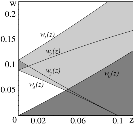
Figure 2: SO-induced extension of the particle-hole continuum shown for $y=0.1$. It is bounded from above by parabola $w_{1}(z)$ [Eq. (49)] and bounded from below by the parabola $w_{4}(z)$ [Eq. (52)] and by the parabola $w_{0}(z)=z^{2}+z$ of the conventional particle-hole (Landau damping) region. The small darkened triangle indicates the region where the approximation $\sigma(z,w)\approx\sigma(0,w)$ is applicable.

An extension of the particle-hole continuum reflects an opened possibility for transitions between SO-split subbands. Therefore one can expect new SO-induced effects of damping of various collective excitations (plasmons, LO phonons) in the new regions of damping. These issues will be discussed in the subsequent sections. Below we present ${\rm Im}\Pi$ in explicit form for the values $w>w_{0}(z)$, i.e., above the boundary $w_{0}(z)$ of the conventional particle-hole continuum. Since $w_{0}(z)>z^{2}+yz$, we deal with the case of the roots’ ordering (45) corresponding to the domain ${\cal C}$. Assuming that $y$ does not exceed the value $\frac{2-\sqrt{2}}{2}\approx 0.3$, we deduce from (III.1),

$$- \frac{1}{\nu}{\rm Im}\Pi=-\Theta(w_{2}(z)-w)\Theta(w-w_{4}(z))\int_{-z-y}^{z-y}\!\!d\tau{\cal L}(\tau)$$

$$- \Theta(w_{1}(z)-w)\Theta(w-w_{2}(z))\int_{-z-y}^{\frac{1}{2}[1-\sqrt{1+4w}]}\!\!d\tau{\cal L}(\tau)$$

$$+ \Theta(w_{3}(z)-w)\Theta(w-w_{4}(z))\int_{-z-y}^{\frac{1}{2}[\sqrt{1-4w}-1]}\!\!\!d\tau{\cal L}(\tau).$$

Applying the table integral (C) for $x_{1}=\tau_{1}$, $x_{a}=x_{2}=\tau_{3}$, $x_{b}=x_{3}=\tau_{4}$, and $x_{4}=\tau_{2}$, we obtain the analytic expression

$$- \!\!\frac{1}{\nu}{\rm Im}\Pi=-\Theta(w_{2}(z)-w)\Theta(w-w_{4}(z))A(z-y)$$

$$- \!\!\Theta(w_{1}(z)-w)\Theta(w-w_{2}(z))A(\frac{1}{2}[1-\sqrt{1+4w}])$$

$$+ \!\!\Theta(w_{3}(z)-w)\Theta(w-w_{4}(z))A(\frac{1}{2}[\sqrt{1-4w}-1]),$$

where

$$w_{1}(z) = (z+y)^{2}+(z+y),$$ (49)

$$w_{2}(z) = (z-y)^{2}-(z-y),$$ (50)

$$w_{3}(z) = -(z+y)^{2}+(z+y),$$ (51)

$$w_{4}(z) = -(z-y)^{2}-(z-y),$$ (52)

and

$$A(x) = \frac{1}{2z}\sqrt{\frac{w-zx}{w+zx}[z^{2}-(x+y)^{2}]}+\frac{k}{4z\sqrt{w}}\times$$ (53)

$$\times [((w/z-y)^{2}-z^{2})F(\varphi(x),k)$$

$$-((w/z+z)^{2}-y^{2})E(\varphi(x),k)$$

$$+2y(w/z-y-z)\Pi(\varphi(x),n,k)].$$

The argument $\varphi(x)$ and the parameters $k$ and $n$ of the elliptic functions $F$, $E$ and $\Pi$ are defined in the following way:

$$\varphi(x) = \arcsin\sqrt{\frac{(x+z+y)(w/z-y+z)}{2(zx+w)}},$$ (54)

$$k = \frac{2\sqrt{w}}{\sqrt{(w/z+z)^{2}-y^{2}}},\quad n=\frac{2z}{w/z+z-y}.$$ (55)

Note that $\varphi(-z-y)=0$ and $\varphi(z-y)=\frac{\pi}{2}$, and hence $A(z-y)$ is expressed in terms of the complete elliptic integrals $F(\frac{\pi}{2},k)$, $E(\frac{\pi}{2},k)$, and $\Pi(\frac{\pi}{2},n,k)$.

III.3 Comparison with the approximate result

It is also worthwhile to compare our exact result (III.2) with an approximation for small $z$ commonly used in the literature (cf., e.g., Refs. MCE, ; MH, ; SL, ). It neglects the square of the transferred momentum $q^{2}$ in the denominator of (5), and therefore leads to the kinematic extension of the conventional particle-hole continuum to a strip $y-y^{2}<w<y+y^{2}$ parallel to the $z$ axis. This approximation can be effectively expressed in the form

$$\Pi(q,\omega)\approx-i\frac{q^{2}}{e^{2}\omega}\sigma(0,\omega),$$ (56)

and considered as stemming from the identity

$$\Pi(q,\omega)=-i\frac{q^{2}}{e^{2}\omega}\sigma(q,\omega),$$ (57)

with $\sigma(q,\omega)$ replaced by $\sigma(0,\omega)$. The optical conductivity $\sigma(0,\omega)\equiv\sigma_{\omega}$ can be easily found MCE . For example, its real part equals

$${\rm Re}\sigma_{\omega}=\frac{e^{2}}{16\pi}\Theta(y^{2}-|w-y|).$$ (58)

Thus, Eq. (56) yields

$$-\frac{1}{\nu}{\rm Im}\Pi\approx\frac{4\pi z^{2}}{e^{2}w}{\rm Re}\sigma_{\omega}=\frac{\pi z^{2}}{4w}\Theta(y^{2}-|w-y|).$$ (59)

We would like to argue that the approximation (59) works well only in a quite small region restricted by the conditions $w_{3}(z)<w<w_{2}(z)$ (see Fig. 2). Since the parabolas $w_{2}(z)$ and $w_{3}(z)$ intersect at $z=\frac{1}{2}[1-\sqrt{1-4y^{2}}]\approx y^{2}$, this region is represented by a small triangle between the points $(0,y-y^{2})$, $(0,y+y^{2})$, $(y^{2},y)$. Inside this triangle $-{\rm Im}\Pi/\nu$ is entirely determined by $-A(z-y)$. Observing that $k^{2}\approx 2n\approx 4z^{2}/w$ for small $z<y^{2}$ and expanding the complete elliptic integrals with respect to $z$, we find an asymptotic value,

$$-A(z-y)\approx\frac{\pi z^{2}}{4w},$$ (60)

which coincides with (59), except for the domain of applicability.

In Fig. 3 we compare the curves $16\pi{\rm Re}[\sigma(z_{c},w)]/e^{2}$ calculated at the different values of $z_{c}$ and $y=0.1$, and plotted as a function of $w$. The unit-step between $y-y^{2}=0.09$ and $y+y^{2}=1.01$ corresponds to the optical conductivity (58), which is recovered at $z_{c}=0$. One can observe that for $z\ll y^{2}$ the approximation $\sigma(z,w)\approx\sigma(0,w)$ leading to (59) works quite well, while for $z\gg y^{2}$ it completely breaks down.

Figure 3: The real part of conductivity for the values of $z_{c}=0.0$, $0.025$, $0.005$, $0.01$, $0.02$, $0.03$, $0.04$ calculated at $y=0.1$. The unit step corresponds to $z_{c}=0$. The dashed line corresponds to $z_{c}=y^{2}=0.01$, which is the limiting value for the applicability of the approximation $\sigma(z,w)\approx\sigma(0,w)$.

IV Static limit of the polarization operator

IV.1 Careful derivation of the static limit

In this section we derive the static limit

$$\lim_{w\to 0}{\rm Re}\Pi(z,w)=\lim_{w\to 0}{\rm Re}\Pi^{I}(z,w)+\lim_{w\to 0}{\rm Re}\Pi^{II}(z,w).$$ (61)

After Eq. (17) we have already made an observation that $\lim_{w\to 0}{\rm Re}\Pi^{II}(z,w)$ might seem to vanish. Below we prove that, in fact, it does not vanish, but rather produces a finite and a very important contribution to $\lim_{w\to 0}{\rm Re}\Pi(z,w)$ for small $z<y$.

Let us first identify the quantity $\lim_{w\to 0}{\rm Re}\Pi^{I}(z,w)$. One can see that if we put $w=0$ in (16), all the roots $\lambda_{i\sigma}$ become real for all values of the integration variable $v$. Tracing back the derivation of the expression (14), it is easy to see that $\lim_{w\to 0}{\rm Re}\Pi^{I}(z,w)$ is obtained, in fact, from the definition (cf. Ref. Raikh, )

$$\widetilde{\Pi}_{q,\omega+i\delta=0}=\sum_{\chi,\mu=\pm}\int\frac{d^{2}{\bf k}}{(2\pi)^{2}}\,\,\frac{n_{F}(\epsilon_{{\bf k}}^{\mu})-n_{F}(\epsilon_{{\bf k}+{\bf q}}^{\chi\mu})}{\epsilon_{{\bf k}}^{\mu}-\epsilon_{{\bf k}+{\bf q}}^{\chi\mu}}{\cal F}^{\chi}_{{\bf k},{\bf k}+{\bf q}}.$$ (62)

We would like to emphasize that, in general, $\widetilde{\Pi}_{q,\omega+i\delta=0}$ is not always the same as $\lim_{\omega\to 0}\Pi_{q\omega}$, and there might occur a specific situation when

$$\lim_{\omega\to 0}\Pi_{q\omega}\neq\widetilde{\Pi}_{q,\omega+i\delta=0}.$$ (63)

Once $\lim_{w\to 0}{\rm Re}\Pi^{II}(z,w)$ is nonzero, the subtle property (63), for example, holds for the 2DEG with Rashba SO coupling described by the Hamiltonian (1).

The correct static limit is, of course, given by $\lim_{\omega\to 0}\Pi_{q\omega}$. However, it is very tempting to put $\omega=0$ from the very beginning. In principle, one can do that. But then, in order to protect oneself from a possible mistake, it is necessary to keep small $\delta\neq 0$ until the very end, even during a calculation of a real part of the polarization operator. More formally, the sequences of operations,

$$\lim_{\omega\to 0}\int d^{2}{\bf k}\lim_{\delta\to 0}\left(\cdots\right)\quad{\rm and}\quad\lim_{\delta\to 0}\int d^{2}{\bf k}\lim_{\omega\to 0}\left(\cdots\right)$$ (64)

always lead to a correct static limit, while the sequence

$$\int d^{2}{\bf k}\lim_{\omega,\delta\to 0}\left(\cdots\right)$$ (65)

might give in some specific cases an unphysical result breaking causality and violating analytic properties of a (retarded) response function.

Let us rigorously prove the statements which have been made previously. In studying the limit $w\to 0$ of ${\rm Re}\Pi={\rm Re}\Pi^{I}+{\rm Re}\Pi^{II}$ it is sufficient to consider how we approach the axis $w=0$ from the domains ${\cal D}$ and ${\cal A}$ (see Fig. 1) that cover the ranges of momenta $z\in(0,y)$ and $z\in(y,+\infty)$, respectively, as $w\to 0$. In turn, the domains ${\cal C}$ and ${\cal B}$ in this limit shrink to the points $z=0$ and $z=y$, and therefore their consideration is not important for our current purpose.

Let us first consider ${\rm Re}\Pi^{I}$ in the domain ${\cal D}$ at very small $w$. In the range of integration $[\tau_{2},\tau_{1}]$ we can replace

$${\cal R}^{\pm}(\tau)\approx{\cal R}_{1}(\tau)\,\,{\rm sign}(\tau\mp wy/z^{2})=\mp{\cal R}_{1}(\tau),$$ (66)

where

$${\cal R}_{1}(\tau)=\frac{1}{2z}\frac{\sqrt{y^{2}-z^{2}}}{\sqrt{(w/z)^{2}-\tau^{2}}}.$$ (67)

Meanwhile, in the range of integration $[\tau_{4},\tau_{3}]$ we have

$${\cal R}^{\pm}(\tau)\approx{\cal R}_{2}(\tau)=-\frac{1}{2z\tau}\sqrt{z^{2}-(\tau+y)^{2}}.$$ (68)

We observe that $\tau_{++}(-)=-\tau_{-+}(+)\approx 1$, $\tau_{++}(+)=-\tau_{-+}(-)\approx w$, $\tau_{++}(y)\approx w/y$, $\tau_{-+}(y)\approx-y$; $\tau_{+-}(-)=-\tau_{--}(+)\approx 1$, $\tau_{--}(-)=-\tau_{+-}(+)\approx w$, $\tau_{+-}(y)\approx-w/y$, $\tau_{--}(y)\approx-y$; $\tau_{++}(0)=-\tau_{-+}(0)=\sqrt{w}$. Taking into account that $z<y$, we carefully arrange the limits of integration, and thus obtain

$$- \frac{1}{\nu}\lim_{w\to 0}{\rm Re}\Pi^{I}=$$ (69)

$$= \left(\int_{-y}^{z-y}+\int_{-y}^{-z-y}+\int_{z-y}^{-z-y}+2\int_{-y}^{z-y}\right)d\tau{\cal R}_{2}(\tau)$$

$$- \lim_{w\to 0}\left(\int_{w/y}^{w/z}+\int_{w/y}^{w}+\int_{-w/z}^{-w}\right)d\tau{\cal R}_{1}(\tau)$$

$$+ \lim_{w\to 0}\left(\int_{w/z}^{w}+\int_{-w/z}^{-w}+2\int_{-w/y}^{-w/z}\right)d\tau{\cal R}_{1}(\tau)$$

$$= 2\left(\int_{-y}^{z-y}\!\!+\int_{-y}^{-z-y}\right)d\tau{\cal R}_{2}(\tau)-\lim_{w\to 0}4\int_{w/y}^{w/z}\!\!d\tau{\cal R}_{1}(\tau)$$

$$= -\int_{0}^{z}\frac{2\tau\sqrt{z^{2}-\tau^{2}}d\tau}{z(\tau^{2}-y^{2})}-\int_{z/y}^{1}\frac{2\sqrt{y^{2}-z^{2}}d\tau}{z\sqrt{1-\tau^{2}}}$$

$$= 2-\frac{\pi}{z}\sqrt{y^{2}-z^{2}},$$

by virtue of the table integral (A).

Let us now consider ${\rm Re}\Pi^{I}$ in the domain ${\cal A}$ at very small $w$. Taking into account that now $z>y$, we obtain

$$- \frac{1}{\nu}\lim_{w\to 0}{\rm Re}\Pi^{I}=\lim_{w\to 0}\left(\int_{w/y}^{\min(1,z-y)}+\int_{w/y}^{\max(w,w/z)}\right.$$ (70)

$$- \int_{-y}^{-\max(w,w/z)}-\int_{-y}^{-\min(1,z+y)}+\int_{\sqrt{w}}^{\min(1,z-y)}$$

$$+ \int_{\sqrt{w}}^{\max(w,w/z)}-\int_{-\sqrt{w}}^{-\max(w,w/z)}-\int_{-\sqrt{w}}^{-\min(1,z+y)}$$

$$- \left.2\int_{-w/y}^{-\sqrt{w}}-2\int_{-y}^{-\sqrt{w}}\right)d\tau{\cal R}(\tau)$$

$$= \lim_{w\to 0}\left(\int_{w/y}^{\max(w,w/z)}-\int_{-w/y}^{-\max(w,w/z)}-\int_{-y}^{-\min(1,z+y)}\right.$$

$$+ \left.\int_{\sqrt{w}}^{\min(1,z-y)}-\int_{-y}^{-\sqrt{w}}\right)d\tau 2{\cal R}(\tau).$$

In the first and the second integrals of the last part of (70), we can replace

$${\cal R}(\tau)\approx{\cal\tilde{R}}_{1}(\tau)=-\frac{1}{2z}\frac{\sqrt{z^{2}-y^{2}}}{\sqrt{\tau^{2}-(w/z)^{2}}},$$ (71)

while in the third integral

$${\cal R}(\tau)\approx{\cal R}_{2}(\tau)\,\,{\rm sign(\tau)}.$$ (72)

The fourth and fifth integrals require a more careful consideration. We note that for small $w$ there holds the inequality $\sqrt{w}>w/z$, which allows us to neglect $w$ in ${\cal R}(\tau)$. Therefore these two integrals can be rewritten as

$$2\lim_{w\to 0}\left(\int_{-y}^{\min(1,z-y)}-\int_{-\sqrt{w}}^{\sqrt{w}}\right)d\tau{\cal R}_{2}(\tau)$$

$$=2\int_{-y}^{\min(1,z-y)}d\tau{\cal R}_{2}(\tau),$$ (73)

where the integral on the rhs of (73) is understood in the sense of principal value.

Thus we obtain for $z>y$

$$- \frac{1}{\nu}\lim_{w\to 0}{\rm Re}\Pi^{I}=-\int_{z/y}^{\max(1,z)}\frac{2\sqrt{z^{2}-y^{2}}d\tau}{z\sqrt{\tau^{2}-1}}$$

$$- \!\!\int_{0}^{\min(1-y,z)}\frac{\sqrt{z^{2}-\tau^{2}}d\tau}{z(\tau+y)}-\int_{0}^{\min(1+y,z)}\frac{\sqrt{z^{2}-\tau^{2}}d\tau}{z(\tau-y)}.$$

It is easy to calculate this expression using the table integral (A). The result is expressed in (109) and (A).

Let us now consider the static limit of ${\rm Re}\Pi^{II}$. In Appendix D we show that it equals

$$-\frac{1}{\nu}\lim_{w\to 0}{\rm Re}\Pi^{II}=\frac{\pi\sqrt{y^{2}-z^{2}}}{z}\Theta(y-z).$$ (75)

We note that this term is nonzero only for $z<y$ (or $q<2k_{R}$). One can observe that (75) is exactly canceled by the counterterm from (69).

Collecting all contributions and introducing $\sin\psi=y/z$ for $y<z$ and $\sin\psi_{\pm}=(1\pm y)/z$ for $1\pm y<z$, we present the static limit of the polarization operator in the form

$$- \frac{1}{\nu}{\rm Re}\Pi(z,0)=2\,\,\Theta(1-y-z)+\Theta(y-|z-1|)\,\,(1+\frac{\pi}{2}\sin\psi)-2\,\Theta(z-1)\,{\rm arccosh}z\,\cos\psi$$ (76)

$$+ \sum_{\mu=\pm}\Theta(z-(1+\mu y))\left(1+\mu\psi_{\mu}\sin\psi-\cos\psi_{\mu}-2\cos\psi\ln\frac{1+z\sin(\psi_{\mu}-\mu\psi)}{2\sqrt{2z}\cos\frac{1}{2}\psi_{\mu}\cos\frac{1}{2}\psi}\right),$$

where ${\rm Re}\Pi(z,0)\equiv\lim_{w\to 0}{\rm Re}\Pi(z,w)$. In what follows we also use the abbreviations ${\rm Re}\Pi^{I}(z,0)$ and ${\rm Re}\Pi^{II}(z,0)$ for $\lim_{w\to 0}{\rm Re}\Pi^{I}(z,w)$ and $\lim_{w\to 0}{\rm Re}\Pi^{II}(z,w)$.

IV.2 Analysis of Eq. (76)

Let us analyze the expression (76). For the values $z<1-y$ we obtain ${\rm Re}\Pi(z,0)=-2\nu$, which ensures the fulfillment of the compressibility sum rule. For $z>1-y$, ${\rm Re}\Pi(z,0)$ deviates from the value $-2\nu$.

Figure 4: The behavior of $-{\rm Re}\Pi(z,0)/\nu$ near $z=1$ for $y=0.1$ (solid line) and $y=0$ (dotted line). The difference between the two curves is shown in the inset.

For $y=0$, Eq. (76) reproduces the conventional result of Stern, Stern

$$-\frac{1}{\nu}{\rm Re}\Pi_{y=0}(z,0)=2-2\sqrt{1-1/z^{2}}\Theta(z-1).$$ (77)

In Fig. 4 we compare $-{\rm Re}\Pi(z,0)/\nu$ for $y=0.1$ and $y=0$. We demonstrate that $-{\rm Re}\Pi_{y\neq 0}(z,0)/\nu$ is always larger than $-{\rm Re}\Pi_{y=0}(z,0)/\nu$, although the difference between the two curves (shown in the inset) is quite small. In particular, the maximal value of $-{\rm Re}\Pi(z,0)/\nu$ at $z=1$ scales with $y$ like

$$-\frac{1}{\nu}{\rm Re}\Pi(1,0)\approx 2+\frac{2\sqrt{2}}{3}y^{3/2},$$ (78)

while at large $z$ the asymptotic behavior of (76) is $\sim\frac{1+y^{2}}{z^{2}}$.

An important test of our results is provided by the Kramers-Kronig relations and the sum rules. For example, using the analytic expressions for ${\rm Re}\Pi(z,0)$ and ${\rm Im}\Pi(z,w)$ we have checked the zero-frequency Kramers-Kronig relation

$${\rm Re}\Pi(z,0) = \frac{2}{\pi}\int_{0}^{\infty}\frac{dw}{w}\,\,{\rm Im}\,\Pi(z,w).$$ (79)

The actual limits of the integration are finite and given by the boundaries of the particle-hole continuum. This has allowed us to confirm (79) numerically with a sufficiently good accuracy (the deviation is $\leq 10^{-6}$ even for a quite simple routine).

Figure 5: The behavior of $-{\rm Re}\Pi(z,0)/\nu$ (solid line) and $-{\rm Re}\Pi^{I}(z,0)/\nu$ (dashed line) near $z=y$ for $y=0.1$.

It is instructive to compare ${\rm Re}\Pi(z,0)$ and ${\rm Re}\Pi^{I}(z,0)$,

$$-\frac{1}{\nu}{\rm Re}\Pi^{I}(z,0)=-\frac{1}{\nu}{\rm Re}\Pi(z,0)-\frac{\pi\sqrt{y^{2}-z^{2}}}{z}\Theta(y-z).$$ (80)

It is obvious that ${\rm Re}\Pi$ does not have any anomaly at $z=y$ (cf. Ref. Raikh, ), while ${\rm Re}\Pi^{I}$ does have it (see Fig. 5). One can also observe that ${\rm Re}\Pi^{I}$ diverges in the limit $z\to 0$ and changes the sign at some value of $z$. Therefore, it cannot be regarded itself as a correct static limit. Otherwise, it would have violated the compressibility sum rule and generated an instability of the medium by virtue of SO coupling.

Thus, we have demonstrated that in order to obtain the correct static limit of the polarization operator for the 2DEG with Rashba SO coupling it is crucially important to follow the thorough definition that implies (64), but not (65). Otherwise, the contribution ${\rm Re}\Pi^{II}(z,0)$ is missing. Being the difference between ${\rm Re}\Pi(z,0)$ and ${\rm Re}\Pi^{I}(z,0)$, it shows up for $z<y$ (or $q<2k_{R}$), and disappears only when $k_{R}$ goes to zero. Therefore, for the conventional 2DEG ($k_{R}=0$) there is no difference between $\Pi_{q,0}$ and $\widetilde{\Pi}_{q,0}$ [and between (64) and (65) as well]. So the property (63) is a peculiar feature of the 2DEG with $k_{R}\neq 0$. We suppose that it might be related to the singularity of the spectrum (2) at $k=0$.

IV.3 Effective interaction: modification of the Friedel $2k_{F}$-oscillations

Let us conveniently rewrite the RPA expression (3) for the dielectric function in terms of $\tilde{r}_{s}=\frac{r_{s}}{2\sqrt{2}}$,

$$\varepsilon(z,w)=1-\frac{\tilde{r}_{s}}{z\nu}\Pi(z,w),$$ (81)

where $r_{s}=\frac{\sqrt{2}m^{*}e^{2}}{k_{F}\varepsilon_{\infty}}$ is the 2D Wigner-Seitz parameter. The latter controls the accuracy of RPA, which becomes better with decreasing $r_{s}$. In the limit $w\to 0$, Eq. (81) describes the static screening of the Coulomb interaction. It is well-known Stern that the singular behavior of the derivative,

$$-\frac{1}{\nu}\frac{d}{dz}\Pi_{y=0}(z,0)\big{|}_{z=1+\alpha}\approx-\sqrt{\frac{2}{\alpha}},$$ (82)

at $z=1+\alpha$ with small $\alpha>0$ gives rise to the Friedel oscillations of a screening potential, their leading asymptotic term being

$$V_{osc}^{y=0}(\rho)=-\frac{2e^{2}k_{F}}{\varepsilon_{\infty}}\cdot\frac{2\tilde{r}_{s}e^{-2k_{F}d}}{[\varepsilon_{y=0}(1,0)]^{2}}\frac{\sin 2k_{F}\rho}{(2k_{F}\rho)^{2}},$$ (83)

where $\rho=\sqrt{x_{1}^{2}+x_{2}^{2}}$, and $d$ is a distance from a probe charge to the 2DEG plane. The SO modification to (83) follows from

$$-\frac{1}{\nu}\frac{d}{dz}\Pi(z,0)\approx-\sqrt{\frac{2}{\alpha}}\cdot\sqrt{1-y^{2}},$$ (84)

and results in

$$V_{osc}(\rho)=-\frac{2e^{2}k_{F}}{\varepsilon_{\infty}}\cdot\frac{2\tilde{r}_{s}e^{-2k_{F}d}}{[\varepsilon_{y=0}(1,0)]^{2}}\frac{\sin 2k_{F}\rho}{(2k_{F}\rho)^{2}}Q(y),$$ (85)

where the factor

$$Q(y)=\sqrt{1-y^{2}}\left[\frac{\varepsilon_{y=0}(1,0)}{\varepsilon(1,0)}\right]^{2}$$ (86)

is always smaller than $1$. It means that due to the SO coupling the amplitude of the Friedel oscillations is diminished (cf. Ref. Raikh, ), although the amount of such decrease is quite small ($\sim 0.5\%$ for $y=0.07$ and $r_{s}=0.2$). We note that due to (78) it is possible to approximate

$$\left[\frac{\varepsilon_{y=0}(1,0)}{\varepsilon(1,0)}\right]^{2}\approx 1-\frac{4\sqrt{2}y^{3/2}}{3(1+2\tilde{r}_{s})}.$$ (87)

Rigourously speaking, it is necessary to take into account in (85) the dependence of $k_{F}$ on $k_{R}$ as well.

The second derivative $\frac{d^{2}}{dz^{2}}\Pi(z,0)$ also diverges at the points $z=1\pm y+0^{+}$, thus contributing to the subleading asymptotic terms of the oscillating potential Raikh .

V Structure factor and SO-induced damping of plasmons

An important quantity which either can be directly observed or enters into expressions for other observable quantities is the structure factor Mahan

$$S(z,w)=-{\rm Im}\left[1/\varepsilon(z,w)\right].$$ (88)

It depends on the Wigner-Seitz parameter $r_{s}$ and contains information about both particle-hole excitations and collective excitations (plasmons). The spectrum of the latter is found from the equation ${\rm Re}\,\varepsilon=0$. For the conventional 2DEG it can be derived on the basis of Ref. Stern, and equalsSingwi

$$w_{pl}(z)=\frac{z(z+2\tilde{r}_{s})}{2\tilde{r}_{s}}\sqrt{\frac{4\tilde{r}_{s}^{2}+4\tilde{r}_{s}z^{3}+z^{4}}{z(z+4\tilde{r}_{s})}}\Theta(z^{*}-z),$$ (89)

where the endpoint of the spectrum $z^{*}$ is the real positive root of the equation $z^{2}(z+4\tilde{r}_{s})=4\tilde{r}_{s}^{2}$. Provided ${\rm Im}\,\varepsilon=0$, the plasmon spectrum is undamped, and the structure factor is $\delta$-peaked at $w=w_{pl}(z)$,

$$S_{pl}(z,w)=\alpha(z)\delta(w-w_{pl}(z)),$$ (90)

with the weight factor $\alpha(z)=\pi[{\rm Re}\,\partial\varepsilon/\partial w|_{w=w_{pl}(z)}]^{-1}$, given by

$$\alpha(z)=\frac{\pi\sqrt{z}[16\tilde{r}_{s}^{4}-z^{4}(z+4\tilde{r}_{s})^{2}]}{2\tilde{r}_{s}\sqrt{(4\tilde{r}_{s}^{2}+4\tilde{r}_{s}z^{3}+z^{4})(z+4\tilde{r}_{s})^{3}}}.$$ (91)

The plasmon spectrum can be visualized on a contour plot of $S(z,w)$ by adding an artificial infinitesimal damping $\delta$ to ${\rm Im}\,\varepsilon$. It becomes very helpful when an exact analytic expression similar to (89) is not known.

In the presence of SO coupling, the structure factor depends on $y$ as well. Solving approximately the equation ${\rm Re}\,\varepsilon=0$ at $y\neq 0$, we can establish how the plasmon spectrum is modified by SO coupling. In fact, we observe that the SO modification of (89) is quite small. Later on, we will comment on how small it is, and explain why this effect is not really important (cf. Ref. wang, ).

A much more important effect is a damping of plasmons generated by SO coupling. As it has been already discussed, SO coupling extends the continuum of the particle-hole excitations up to the new boundaries shown in Fig. 2. Therefore, the plasmon spectrum is expected to acquire a finite width, whenever it enters into the SO-induced region of damping.

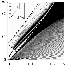
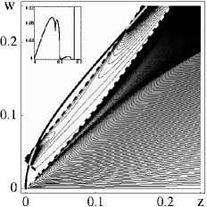
Figure 6: Contour plots of $S(z,w)$ showing the SO-induced wedge-shaped damping region (bounded by the dashed lines). The plasmon mode is depicted by the bold line. Insets show the cross-sections $S(z=0.1,w)$ as a function of $w$. Left panel: $y\!=\!0.07$, $r_{s}\!=\!0.2$. Right panel: $y\!=\!0.04$, $r_{s}\!=\!0.6$.

In Fig. 6 we show the contour-plots of the structure factor $S(z,w)$ depicting the plasmon spectrum by the bold line, in black, where ${\rm Im}\,\varepsilon=0$ (undamped plasmon, the structure factor is $\delta$-peaked) and in gray, where ${\rm Im}\,\varepsilon\neq 0$ (SO-damped plasmon, the structure factor has a finite height and width). Depending on the values of $r_{s}$ and $y$, the two different cases are possible: (I) the plasmon enters only once into the SO-induced damping region (left panel); (II) it enters twice, escaping for a while after the first entrance (right panel).

Within the conventional boundaries $w=z^{2}\pm z$ of the particle-hole continuum, the structure factor $S(z,w)$ is modified by SO coupling only slightly and can be approximated by the conventional expressionsStern .

In the SO-induced region of damping, $S(z,w)$ is very well approximated by the Lorentzian function describing the SO-damped plasmon with the width $\gamma(z)$,

$$S(z,w)_{SO-damp\,\,pl}=\frac{\alpha(z)}{\pi}\frac{\gamma(z)}{(w-w_{pl}(z))^{2}+\gamma^{2}(z)},$$ (92)

where $w_{pl}(z)$ and $\alpha(z)$ are supposed to be practically independent of $y$ and therefore given by (89) and (91), while

$$\gamma(z)=\frac{\alpha(z)}{\pi}{\rm Im}\,\varepsilon(z,w_{pl}(z))$$ (93)

essentially depends on $y$ via ${\rm Im}\,\varepsilon\neq 0$. In Fig. 7 we present the enlarged plot with the cross section $S(z=0.1,w)$ from the inset of the left panel of Fig. 6 and compare it with the approximate $S(0.1,w)_{SO-damp\,\,pl}$ given by (92). The inset of Fig. 7 shows both curves on a more fine scale. Comparing the positions of their peaks, we conclude that the shift of the plasmon dispersion due to SO coupling from $w_{pl}(z)$ (89) is one or two orders of magnitude smaller than $\gamma(z)$ [unless $\gamma(z)=0$], and therefore can hardly be resolved experimentally. The almost equal height of the peaks confirms that (91) is also a very good approximation for the weight factor at $y\neq 0$.

Figure 7: The cross section $S(z=0.1,w)$ (solid line) compared to the approximation $S(z=0.1,w)_{SO-damp\,\,pl}$ (dashed line). Parameters: $y\!=\!0.07$, $r_{s}\!=\!0.2$.

Let us find the values of $y$ and $r_{s}$ that correspond to the typical cases (I) and (II) shown in the left and right panels of Fig. 6, respectively. For this purpose, it is necessary to establish when the curves $w_{1}(z)$ (49) and $w_{pl}(z)$ (89) touch each other. The result is represented in Fig. 8, where the plane $(y,r_{s})$ is divided into the corresponding domains I and II. Changing $y$ and $r_{s}$, we can tune the relative position of the SO-induced particle-hole continuum and the plasmon spectrum. The insets show $\overline{\gamma}(z)=\gamma(z)\times 10^{4}$ for the values of parameters the same as in Fig. 6: (I) $y=0.07$, $r_{s}=0.2$; (II) $y=0.04$, $r_{s}=0.6$. The function $\gamma(z)$ is defined for $z\leq z^{*}$ and vanishes where the plasmon is undamped.

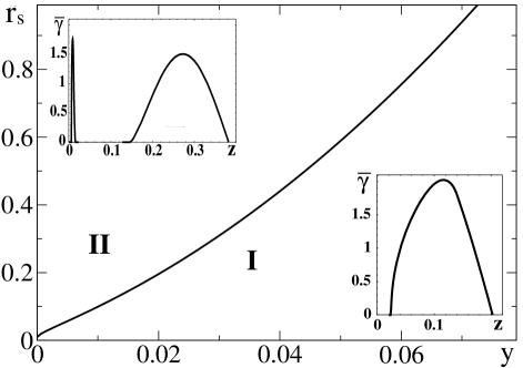
Figure 8: The plane $(y,r_{s})$ is divided into the domains I and II, where the plasmon has one or two undamped pieces, respectively (cf. Fig. 6). Insets show SO-induced plasmon width $\overline{\gamma}(z)=\gamma(z)\times 10^{4}$ for the same parameters as in Fig. 6.

A direct measurement of SO-induced plasmon width can be provided by means of inelastic light (Raman) scattering (see, e.g., Ref. Raman, ). Experimentally it is possible to measure the structure factor in the range $q=0-2\times 10^{7}$m^-1 which corresponds to the range of $z=0-0.1$ (for $r_{s}\sim 1$). Keeping $z$ at a fixed value and varying $y$ and $r_{s}$, one should observe different patterns of $S(z,w)$ with either damped or undamped plasmon, like those shown in the insets to Fig. 6, where the sections of $S(z,w)$ at constant $z=0.1$ are presented. In order to estimate realistic parameters, we focus on InAs-based 2DEG, where the strength of Rashba coupling $\alpha_{R}$ has quite large values up to $\sim 3\times 10^{-11}$eVm (Ref. large, ) and prevails over the Dresselhaus term Ganichev . Most of experiments deal with the 2DEG’s densities ranging from $n=0.7\times 10^{16}$m^-2 (Ref. Engels, ) to $n=2.4\times 10^{16}$m^-2 (Ref. Nitta, ). Taking $\varepsilon_{\infty}\approx 12$ and $m^{*}\approx 0.03m_{e}$, we obtain the range of $y$ from 0.04 to 0.075 and the range of $r_{s}$ from 0.38 to 0.3. These values belong to the domain I in Fig. 8, where the SO-damping of the plasmon is especially important. Choosing the value of $\gamma\sim 10^{-4}$, we establish that $2\tau_{pl}=\hbar/(4\gamma E_{F})$ is of the order of 10 ps. This can, in principle, be resolved experimentally, since the Raman measurements done in II-VI quantum wells Jus give a finite lifetime of the plasmon mode with the typical value $2\tau_{pl}\sim 0.3$ ps. We also point out that the II-VI compounds (e.g., HgTe) represent an even more promising candidate for observation of the discussed effects since the reported SO coupling strength is comparatively largeMol .

Plasmon broadening may be also caused by thermal effects. We use the results for 2DEG at finite temperature Fetter in order to estimate the relative contributions of SO-induced and thermal damping. The former dominates over the latter below some characteristic temperature that is about 90 K for the parameters of Ref. large, . This estimate is made at constant $z=0.1$. Note that the thermal damping strongly depends on the values of $r_{s}$ and temperature, whereas the SO-induced damping has quite a weak $r_{s}$ dependence (e.g., compare the insets in Fig. 8). This may provide a guide for an experimental separation of these two sources of broadening.

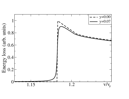
Figure 9: The plasmon contribution to the energy-loss function at $y=0$ (dashed line) compared with the SO-damped plasmon contribution at $y=0.07$ (solid line). For the both curves $r_{s}=0.2$.

A finite lifetime of plasmons would modify the energy-loss function. The energy loss per unit length for a particle moving toward a plane with 2DEG with velocity $v$ is given by

$$-\frac{dW}{dx}=C\left(\frac{v_{F}}{v}\right)\int_{0}^{\infty}zdz\int_{0}^{v/v_{F}}\frac{uS(z,uz)du}{\sqrt{(v/v_{F})^{2}-u^{2}}},$$ (94)

where $C=16\pi^{2}e^{2}n/\varepsilon_{\infty}$. In the presence of SO coupling, the most essential modification is expected in the plasmon sector. In Fig. 9 we plot the plasmon contributions $(-dW/dx)_{pl}$ for $y=0$ and $y=0.07$ as a function of $v/v_{F}$. Both curves are calculated at $r_{s}=0.2$ and normalized by the peak value of $(-dW/dx)_{pl}$ at $y=0$. We observe that the sharp peak is smoothed down and the steplike behavior becomes more smeared with increasing SO coupling strength.

VI SO-induced damping of LO phonons

Our results for the structure factor allow us to predict that the other collective mode, longitudinal optical (LO) phonon, will also experience a pronounced SO-induced damping. Its dispersion and lifetime can be obtained from the renormalized propagator that is expressed in RPA as JS

$$D(q,\omega)=\frac{2\omega_{LO}}{\omega^{2}-\omega^{2}_{LO}-2\omega_{LO}M_{q}^{2}\Pi_{q\omega}/\varepsilon_{q\omega}},$$ (95)

where $M_{q}^{2}=\textstyle{\frac{1}{2}}\kappa V_{q}\omega_{LO}$, and $\kappa=1-\varepsilon_{\infty}/\varepsilon_{0}$ is a material parameter. On the basis of this expression, we can establish that the LO-phonon width (normalized by $2k_{F}^{2}/m^{*}$) equals

$$\gamma_{LO}(z)=\frac{\kappa S(z,w)(w_{0}{\rm Re}\,\varepsilon)^{2}}{2w({\rm Re}\,\varepsilon)^{2}+\kappa w_{0}^{2}{\rm Re}(\partial\varepsilon/\partial w)}\bigg{|}_{w=w_{ph}(z)},$$ (96)

where $w_{0}=(m^{*}/2k_{F}^{2})\,\,\omega_{LO}$ and $w_{ph}(z)$ is the renormalized phonon spectrum. Like in the case of plasmons, we may neglect the dependence of $w_{ph}(z)$ on SO coupling, and find the phonon spectrum from the equation $w^{2}=w_{0}^{2}[1+\kappa(({\rm Re}\,\varepsilon)^{-1}-1)]$, where ${\rm Re}\,\varepsilon$ is taken at $y=0$.

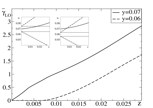
Figure 10: SO-induced damping of the LO phonon $\overline{\gamma}_{LO}(z)=\gamma_{LO}(z)\times 10^{4}$ for $w_{0}=0.07$, $r_{s}=0.4$, $\varepsilon_{\infty}=12$, and $\varepsilon_{0}=15$. Solid and dashed lines correspond to the cases $y=0.07$ ($|w_{0}-y|<y^{2}$) and $y=0.06$ ($|w_{0}-y|>y^{2}$), respectively. Insets show the location of the phonon spectrum (solid line) relative to the SO-induced damping region (dashed lines) and to the strip $y-y^{2}<w<y+y^{2}$ (dotted lines) for $y=0.07$ (left) and $y=0.06$ (right).

The lifetime effects of the LO phonons can be very important for a coupled dynamics of carriers and phonons. An interesting possibility arises when $\omega_{LO}\sim 2\alpha_{R}k_{F}$ (or $w_{0}\sim y$). This, for example, holds in InAs, where the value $\omega_{LO}\approx 28$ meV gives $w_{0}\approx 0.07$. Changing the Rashba coupling strength $\alpha_{R}$ by an applied electric field, one can manipulate the lifetime of an optical phonon, which would result in a modification of transport properties by virtue of the electron-phonon coupling.

In Fig. 10 we show the function $\overline{\gamma}_{LO}(z)=\gamma_{LO}(z)\times 10^{4}$. In our calculations we used the following parameters: $w_{0}=0.07$, $r_{s}=0.4$, $\varepsilon_{\infty}=12$, and $\varepsilon_{0}=15$ (for InAs). Choosing the value $\gamma_{LO}=10^{-4}$, we find that for LO phonons the SO-induced lifetime $2\tau_{LO}$ is of the order of 10 ps as well. We note that the typical lifetime for the LO phonons measured in AlAs and GaAs by the Raman spectroscopy is of the same order LOphonon . One can observe that for $y=0.07$ ($|w_{0}-y|<y^{2}$) the damping is always finite (solid line), while for $y=0.06$ ($|w_{0}-y|>y^{2}$) it becomes nonzero only after some value $z\approx 0.007$ (dashed line). In the two insets we show the relative location of the phonon spectrum (solid line) and of the SO-induced damping region (dashed lines). We also depict the boundaries of the strip $w=y\pm y^{2}$ (dotted lines), and one can see that for $y=0.07$ the phonon spectrum leaves it at the value $z\approx 0.017$ (left inset), while for $y=0.06$ the phonon spectrum never gets inside the strip (right inset). This indicates that the the approximation (59) is insufficient for describing the discussed effect.

VII Conclusion

We have calculated the dielectric function of 2DEG with Rashba SO coupling in RPA at zero temperature. We have described the new features of screening that appear due to SO coupling. In particular, we have discussed in detail the extension of the region of the particle-hole excitations, which leads, in turn, to the additional broadening of the plasmon mode. The same mechanism generates the SO-induced lifetime of the longitudinal optical phonons. Speaking generally, we have seen how SO coupling tends to suppress collective excitations due to the relaxation via intersubband transitions. At the same time, SO coupling does not affect much the position of the collective mode dispersions, and therefore this effect is less important.

Another conclusion that can be derived from our studies is that the 2DEG with Rashba SO coupling requires a more careful treatment as far as various approximations are concerned. Usually they fall into the following categories: (1) the so-called $\xi$-approximation based on the linearization of the spectrum; (2) an expansion of physical quantities in powers of SO-coupling strength before their evaluation; (3) reshuffling the operations of the momentum integration and taking the limit of zero frequency. The examples that indicate that none of these approximations provide a fully reliable result for the system in question are the following: (1) being a version of the $\xi$-approximation, Eq. (56) has a very limited range of applicability; (2) the static polarization operator at small $y$ cannot be obtained by means of the power expansion in $y$, because its maximal value scales as $y^{3/2}$ [see Eq. (78)]; (3) reshuffling the order of operations leads to the unphysical result with violated analytic properties. Although the underlying reason of the failure is not quite clear, the above examples warn against the blind usage of these popular approximations in this system.

Finally, the comparison of our theoretical estimates for SO-induced lifetimes of plasmon and LO-phonons with the values of the recent Raman scattering measurements suggests that the effects described above can be observed experimentally.

VIII Acknowledgements

We are grateful to Dionys Baeriswyl, Gerd Schön, and Emmanuel Rashba for valuable discussions. M.P. was supported by the Deutsche Forschungsgemeinschaft (DFG). V.G. was supported by the Swiss National Science Foundation through Grant No. 20-68047.02.

Appendix A Some technical details of the derivation of $\Pi(q,\omega)$

Intermediate steps that lead from from (10) to (11)-(14) are to express

$$g_{i}(v,z,w,y) = \frac{\lambda}{4}\int_{0}^{2\pi}d\phi\left[\left(1+\frac{v+2zx}{|{\bf v}+2{\bf z}|}\right)\delta(2\lambda w-2z^{2}-2vzx+\mu vy-\mu y|{\bf v}+2{\bf z}|)\right.$$ (97)

$$\left.\qquad+\left(1-\frac{v+2zx}{|{\bf v}+2{\bf z}|}\right)\delta(2\lambda w-2z^{2}-2vzx+\mu vy+\mu y|{\bf v}+2{\bf z}|)\right],$$

$$f_{i}(v,z,w,y) = \int_{0}^{2\pi}\frac{d\phi}{\pi}\frac{vzx+z^{2}-\mu y(zx+v)-\lambda w}{(2vzx+2z^{2}-\mu yv-2\lambda w)^{2}-y^{2}(v^{2}+4z^{2}+4vzx)}.$$ (98)

The change of variables (34) implies

$$v = -\frac{\tau^{2}+y\tau-\lambda w}{\mu\tau},$$ (99)

$$\frac{\sigma dv}{v} = -\mu z\frac{d\tau}{y\tau}(\lambda_{i+}-\lambda_{i-}),$$ (100)

$$\lambda_{i\sigma} = \mu\frac{\tau z-\lambda w(\tau+y)/z}{\tau^{2}+y\tau-\lambda w},$$ (101)

$$\lambda_{i\sigma}^{2}-1 = -\frac{\prod_{k=1}^{4}(\tau-\tau_{k})}{(\tau^{2}+y\tau-\lambda w)^{2}},$$ (102)

$$v^{2}C_{i}(\lambda_{i\sigma}+\delta_{i}) = \frac{y\tau}{2z^{2}}\frac{(\tau-\tau_{3})(\tau-\tau_{4})}{\tau^{2}+y\tau-\lambda w},$$ (103)

where $\lambda_{i\sigma}$ are defined in (16), and $C_{i}$ and $\tau_{k}$ are given by (15) and (37), respectively.

In this Appendix we also quote table integrals that we use in our calculations. They can be either found in Ref. gradst, or elaborated on its basis. We quote the standard integral (104) containing the $\delta$-function as well,

$$\int_{0}^{2\pi}d\phi\delta(a+\cos\phi)=\frac{2}{\sqrt{1-a^{2}}}\Theta(1-|a|),$$ (104)

$$\int_{0}^{2\pi}\frac{d\phi}{a+\cos\phi}=\frac{2\pi}{\sqrt{a^{2}-1}}\Theta(|a|-1){\rm sign}(a),$$ (105)

$$\int_{0}^{2\pi}d\phi\frac{x+\delta}{x^{2}+\beta x+\gamma}=\frac{\pi\sqrt{2}}{\sqrt{(1+\gamma)^{2}-\beta^{2}}}$$ (106)

$$\times\frac{(\delta+1)\sqrt{1-\beta+\gamma}+(\delta-1)\sqrt{1+\beta+\gamma}}{\sqrt{\sqrt{(1+\gamma)^{2}-\beta^{2}}+\gamma-1}},\quad(4\gamma>\beta^{2})$$

$$\int\frac{d\tau}{\tau-a}\frac{\sqrt{a^{2}-1}}{\sqrt{1-\tau^{2}}}$$

$$= 2\arctan\frac{a-\tau+a\sqrt{1-\tau^{2}}}{\tau\sqrt{a^{2}-1}},\quad(|\tau|<1<|a|)$$

$$\int\frac{d\tau}{\tau-a}\frac{\sqrt{1-a^{2}}}{\sqrt{1-\tau^{2}}}$$

$$= {\rm ln}\left|\frac{(a-\tau+a\sqrt{1-\tau^{2}}-\tau\sqrt{1-a^{2}})^{2}}{2a(a-\tau)(1+\sqrt{1-\tau^{2}})}\right|,\quad(|\tau|,|a|<1).$$

Using (A) it is easy to establish that

$$-\int_{z/y}^{\max(1,z)}\frac{2\sqrt{z^{2}-y^{2}}d\tau}{z\sqrt{\tau^{2}-1}}\qquad\qquad$$ (109)

$$=-2\sqrt{1-\frac{y^{2}}{z^{2}}}\left[\Theta(z-1){\rm arccosh}z-{\rm arccosh}\frac{z}{y}\right],$$

and

$$- \int_{0}^{\min(1\mp y,z)}\frac{\sqrt{z^{2}-\tau^{2}}d\tau}{z(\tau\pm y)}=1-\Theta(1\mp y-z)$$

$$\times\left[\sqrt{1-\frac{y^{2}}{z^{2}}}\ln\frac{z+\sqrt{z^{2}-y^{2}}}{y}\pm\frac{\pi y}{2z}\right]$$

$$- \Theta(z-(1\mp y))\left[\sqrt{1-\frac{(1\mp y)^{2}}{z^{2}}}\pm\frac{y}{z}\arcsin\frac{1\mp y}{z}\right.$$

$$+ \left.2\sqrt{1-\frac{y^{2}}{z^{2}}}\ln\frac{1\pm y\sqrt{1-\frac{(1\mp y)^{2}}{z^{2}}}+(1\mp y)\sqrt{1-\frac{y^{2}}{z^{2}}}}{\sqrt{2y\left(1+\sqrt{1-\frac{(1\mp y)^{2}}{z^{2}}}\right)}}\right].$$

Appendix B An alternative representation of $f_{3,4}^{II}$

For $4\gamma_{i}>\beta_{i}^{2}$ ($i=3,4$) the roots of the equation $x^{2}+\beta_{i}x+\gamma_{i}=0$ are complex. Omitting the index $i$ (in order to avoid confusion with imaginary $i$), we write them in the form ($\sigma=\pm$)

$$\lambda_{\sigma}=-\frac{\beta}{2}+i\sigma\sqrt{\gamma-\frac{\beta^{2}}{4}},$$ (111)

and note that $\lambda_{-}=\lambda_{+}^{*}$, $|\lambda_{\sigma}|^{2}=\gamma$. The functions $f_{3,4}^{II}\equiv f$ are then represented by

$$f = -\frac{iC}{2\pi(\lambda_{+}-\lambda_{-})}\sum_{\sigma}{\rm sign}\,(\sigma)\frac{\lambda_{\sigma}+\delta}{\sqrt{\lambda_{\sigma}^{2}-1}}$$ (112)

$$\times \oint_{|z|=1}\left(\frac{dz}{z-z_{\sigma+}}-\frac{dz}{z-z_{\sigma-}}\right),$$

where the secondary roots ($\sigma^{\prime}=\pm$)

$$z_{\sigma\sigma^{\prime}}=\lambda_{\sigma}+\sigma^{\prime}\sqrt{\lambda_{\sigma}^{2}-1}$$ (113)

obey the equation $z_{\sigma\sigma^{\prime}}^{2}-2\lambda_{\sigma}z_{\sigma\sigma^{\prime}}+1=0$. Note the properties $z_{-\sigma^{\prime}}=z_{+\sigma^{\prime}}^{*}$ and $z_{\sigma+}z_{\sigma-}=1$. We also denote $z_{++}=e^{a+ib}$, where $a$ and $b$ are real.

Checking which of the roots $z_{\sigma\sigma^{\prime}}$ lie inside the unit circle $|z|=1$, we find an expression for (112),

$$f = -\frac{C\,{\rm sign}(a)}{\lambda_{+}-\lambda_{-}}\left[\frac{\lambda_{+}+\delta}{\sqrt{\lambda_{+}^{2}-1}}-\frac{\lambda_{-}+\delta}{\sqrt{\lambda_{-}^{2}-1}}\right]$$ (114)

$$= -\frac{C\,{\rm sign}(a)}{{\rm Im}\lambda_{+}}{\rm Im}\frac{\lambda_{+}+\delta}{\sqrt{\lambda_{+}^{2}-1}}.$$

One can notice that it resembles its $f^{I}$-counterpart (21), and therefore a (complex) change of variables similar to (34) would lead to the form of integrand the same as in (III.1). However, the corresponding mapping of the integration contour would assume that an integration variable $\tau$ runs in the complex plane along the circle of the radius $\sqrt{w}$. This would probably require an analytic continuation of the elliptic functions (see Appendix C), which makes very cumbersome an explicit representation of (22).

Appendix C Integrals expressed in terms of elliptic functions

Let us consider the integral

$$I=\int\frac{(x-x_{a})(x-x_{b})}{\sqrt{\prod_{k=1}^{4}(x-x_{k})}}dx,$$ (115)

assuming that $x_{4}<x_{3}<x_{2}<x_{1}$. We introduce the notations $x_{rs}=x_{s}-x_{r}$ and

$$k^{2}=\frac{x_{32}x_{41}}{x_{31}x_{42}}.$$ (116)

Let us consider the intervals where the polynomial $\prod_{k=1}^{4}(x-x_{k})$ is positively defined. For $x<x_{4}$ and $x_{1}<x$ the integral (115) equals

$$I =\pm\sqrt{\frac{(x-x_{1})(x-x_{3})(x-x_{4})}{x-x_{2}}}$$

$$+ \frac{1}{\sqrt{x_{31}x_{42}}}[(2x_{a2}x_{b2}+x_{42}x_{21})F(\varphi,k)-x_{31}x_{42}E(\varphi,k)$$

$$+ x_{21}(2x_{a2}+2x_{b2}-x_{32}-x_{42}+x_{21})\Pi(\varphi,\frac{x_{41}}{x_{42}},k)],$$

where

$$\varphi=\arcsin\sqrt{\frac{x_{42}}{x_{41}}\frac{x-x_{1}}{x-x_{2}}},$$ (118)

and the sign “$+$” has to be chosen for $x_{1}<x$, while the sign “$-$” has to be chosen for $x<x_{4}$.

For $x_{3}<x<x_{2}$

$$I =\sqrt{\frac{(x_{1}-x)(x_{2}-x)(x-x_{3})}{x-x_{4}}}$$

$$+ \frac{1}{\sqrt{x_{31}x_{42}}}[(2x_{a4}x_{b4}-x_{42}x_{43})F(\varphi,k)-x_{31}x_{42}E(\varphi,k)$$

$$+ x_{43}(2x_{a4}+2x_{b4}+x_{43}+x_{42}+x_{41})\Pi(\varphi,\frac{x_{32}}{x_{42}},k)],$$

where

$$\varphi=\arcsin\sqrt{\frac{x_{42}}{x_{32}}\frac{x-x_{3}}{x-x_{4}}}.$$ (120)

The elliptic functions

$$F(\varphi,k) = \int_{0}^{\varphi}\frac{d\alpha}{\sqrt{1-k^{2}\sin^{2}\alpha}},$$ (121)

$$E(\varphi,k) = \int_{0}^{\varphi}d\alpha\sqrt{1-k^{2}\sin^{2}\alpha}\ ,$$ (122)

$$\Pi(\varphi,n,k) = \int_{0}^{\varphi}\frac{d\alpha}{(1-n\sin^{2}\alpha)\sqrt{1-k^{2}\sin^{2}\alpha}},$$ (123)

are defined according to Ref. gradst, .

Appendix D Static limit of ${\rm Re}\Pi^{II}$

We start out from the expressions (22) and (III.1). For small $w<y^{2}/4$, we need to consider only the contribution from the function $f_{3}^{II}$ specified by $\mu=-$, i.e.,

$$-\frac{1}{\nu}\lim_{w\to 0}{\rm Re}\Pi^{II}=\lim_{w\to 0}\int_{y-2\sqrt{w}}^{y+2\sqrt{w}}vf_{3}^{II}(v,z,w,y)dv.$$ (124)

Let us introduce a new integration variable $\xi=\frac{v-y}{2\sqrt{w}}$ in (124). Thus, we make the limits of integration independent of $w$, and at this stage it becomes possible to exchange the operation $\lim_{w\to 0}$ and the integration over $\xi$:

$$-\frac{1}{\nu}\lim_{w\to 0}{\rm Re}\Pi^{II} = \lim_{w\to 0}\int_{-1}^{1}d\xi\phi(\xi,z,w,y)$$ (125)

$$= \int_{-1}^{1}\phi_{0}(\xi,z,y)d\xi,$$

where

$$\phi(\xi,z,w,y) = 2\sqrt{w}(y+2\xi\sqrt{w})$$ (126)

$$\times f_{3}^{II}(y+2\xi\sqrt{w},z,w,y),$$

$$\phi_{0}(\xi,z,y) = \lim_{w\to 0}\phi(\xi,z,w,y).$$ (127)

We observe that

$$\sqrt{P_{-}}=\sqrt{z}|z-y|\left[1-\frac{\xi y}{z(z-y)}\sqrt{w}\right.$$

$$+\left.\frac{z^{2}+(z-y)^{2}-\xi^{2}(y^{2}+4z(z-y))}{2z^{2}(z-y)^{2}}w+O(w^{3/2})\right],\quad$$ (128)

$$\sqrt{Q_{-}}=\sqrt{z}(z+y)\left[1-\frac{\xi y}{z(z+y)}\sqrt{w}\right.$$

$$+\left.\frac{z^{2}+(z+y)^{2}-\xi^{2}(y^{2}+4z(z+y))}{2z^{2}(z+y)^{2}}w+O(w^{3/2})\right].\quad$$ (129)

For $z>y$,

$$\sqrt{P_{-}}+\sqrt{Q_{-}} \approx 2z\sqrt{z},$$ (130)

$$\left(\sqrt{P_{-}}+\sqrt{Q_{-}}\right)^{2}-4y^{2}z \approx 4z(z^{2}-y^{2}),$$ (131)

and therefore $\phi_{0}(\xi,z,y)=0$. For $z<y$,

$$\sqrt{P_{-}}+\sqrt{Q_{-}} \approx 2y\sqrt{z},$$ (132)

$$\left(\sqrt{P_{-}}+\sqrt{Q_{-}}\right)^{2}-4y^{2}z \approx \frac{4y^{4}(1-\xi^{2})}{z(y^{2}-z^{2})}w,$$ (133)

and therefore

$$\phi_{0}(\xi,z,y) = \frac{\sqrt{y^{2}-z^{2}}}{z\sqrt{1-\xi^{2}}}.$$ (134)

When inserted in (125), it yields (75).

References

- (1) T. Ando, A. Fowler, and F. Stern, Rev. Mod. Phys. 54, 437 (1982).
- (2) G. D. Mahan, Many-Particle Physics (Plenum Press, New York, 1990).
- (3) F. Stern, Phys. Rev. Lett. 18, 546 (1967).
- (4) S. J. Allen, Jr., D. C. Tsui, and R. A. Logan, Phys. Rev. Lett. 38, 980 (1977).
- (5) T. Nagao, T. Hildebrandt, M. Henzler, and S. Hasegawa, Phys. Rev. Lett. 86, 5747 (2001).
- (6) C. F. Hirjibehedin, A. Pinczuk, B. S. Dennis, L. N. Pfeiffer, and K. W. West, Phys. Rev. B 65, 161309(R) (2002).
- (7) I.V. Kukushkin, J. H. Smet, S. A. Mikhailov, D. V. Kulakovskii, K. von Klitzing, and W. Wegscheider, Phys. Rev. Lett. 90, 156801 (2003).
- (8) I. Žutić, J. Fabian, and S. Das Sarma, Rev. Mod. Phys. 76, 323 (2004); R. H. Silsbee, J. Phys.: Condens. Matter 16, R179 (2004).
- (9) Y.A. Bychkov and E.I. Rashba, J. Phys. C 17, 6039 (1984).
- (10) J. Nitta, T. Akazaki, H. Takayanagi, and T. Enoki, Phys. Rev. Lett. 78, 1335 (1997); Y. Kato, R.C. Myers, A.C. Gossard, and D.D. Awschalom, Nature 427, 50 (2004).
- (11) S. Murakami, N. Nagaosa, and S. C. Zhang, Science 301, 1348 (2003); J. Sinova et al., Phys. Rev. Lett. 92, 126603 (2004).
- (12) G.-H. Chen and M. E. Raikh, Phys. Rev. B 59, 5090 (1999).
- (13) L.I. Magarill, A.V. Chaplik, and M.V. Éntin, JETP 92, 153 (2001).
- (14) E. G. Mishchenko and B. I. Halperin, Phys. Rev. B 68, 045317 (2003).
- (15) X. F. Wang, Phys. Rev. B 72, 085317 (2005).
- (16) D. S. Saraga and D. Loss, Phys. Rev. B 72, 195319 (2005).
- (17) I. S. Gradshteyn and I. M. Ryzhik, Table of Integrals, Series, and Products (Academic, New York, 1994).
- (18) A. Czachor, A. Holas, S. R. Sharma, and K. S. Singwi, Phys. Rev. B 25, 2144 (1982).
- (19) B. Jusserand et al., Phys. Rev. Lett. 69, 848 (1992).
- (20) D. Grundler, Phys. Rev. Lett. 84, 6074 (2000).
- (21) S. D. Ganichev et al., Phys. Rev. Lett. 92, 256601 (2004).
- (22) G. Engels, J. Lange, Th. Schäpers, and H. Lüth, Phys. Rev. B 55, (R)1958 (1997).
- (23) B. Jusserand et al., Phys. Rev. B 63, 161302 (2001).
- (24) Y. S. Gui, et.al., Phys. Rev. B 70, 115328 (2004).
- (25) A. L. Fetter, Phys. Rev. B 10, 3739 (1974); P. M. Platzman and N. Tzoar, Phys. Rev. B 13, 3197 (1976).
- (26) R. Jalabert and S. Das Sarma, Phys. Rev. B 40, 9723 (1989).
- (27) M. Canonico et al., Phys. Rev. Lett. 88, 215502 (2002).