Basic Types of Coarse-Graining

Abstract

We consider two basic types of coarse-graining: the Ehrenfests’ coarse-graining and its extension to a general principle of non-equilibrium thermodynamics, and the coarse-graining based on uncertainty of dynamical models and $\varepsilon$-motions (orbits). Non-technical discussion of basic notions and main coarse-graining theorems are presented: the theorem about entropy overproduction for the Ehrenfests’ coarse-graining and its generalizations, both for conservative and for dissipative systems, and the theorems about stable properties and the Smale order for $\varepsilon$-motions of general dynamical systems including structurally unstable systems. Computational kinetic models of macroscopic dynamics are considered. We construct a theoretical basis for these kinetic models using generalizations of the Ehrenfests’ coarse-graining. General theory of reversible regularization and filtering semigroups in kinetics is presented, both for linear and non-linear filters. We obtain explicit expressions and entropic stability conditions for filtered equations. A brief discussion of coarse-graining by rounding and by small noise is also presented.

1 Introduction

Almost a century ago, Paul and Tanya Ehrenfest in their paper for scientific Encyclopedia Ehrenfest introduced a special operation, the coarse-graining. This operation transforms a probability density in phase space into a “coarse-grained” density, that is a piece-wise constant function, a result of density averaging in cells. The size of cells is assumed to be small, but finite, and does not tend to zero. The coarse-graining models uncontrollable impact of surrounding (of a thermostat, for example) onto ensemble of mechanical systems.

To understand reasons for introduction of this new notion, let us take a phase drop, that is, an ensemble of mechanical systems with constant probability density localized in a small domain of phase space. Let us watch evolution of this drop in time according to the Liouville equation. After a long time, the shape of the drop may be very complicated, but the density value remains the same, and this drop remains “oil in water.” The ensemble can tend to the equilibrium in the weak sense only: average value of any continuous function tends to its equilibrium value, but the entropy of the distribution remains constant. Nevertheless, if we divide the phase space into cells and supplement the mechanical motion by the periodical averaging in cells (this is the Ehrenfests’ idea of coarse-graining), then the entropy increases, and the distribution density tends uniformly to the equilibrium. This periodical coarse-graining is illustrated by Fig. 1 for one-dimensional (1D) and two-dimensional (2D) phase spaces.

a)

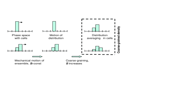
b)

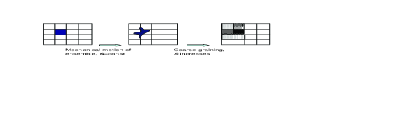
Figure 1: The Ehrenfests’ coarse-graining: two “motion – coarse-graining” cycles in 1D (a, values of probability density are presented by the height of the columns) and one such cycle in 2D (b, values of probability density are presented by hatching density).

Recently, we can find the idea of coarse-graining everywhere in statistical physics (both equilibrium and non-equilibrium). For example, it is the central idea of the Kadanoff transformation, and can be considered as a background of the Wilson renormalization group Wilson and modern renormalisation group approach to dissipative systems RG ; Kun3 . It gave a simplest realization of the projection operators technique Grabert long before this technic was developed. In the method of invariant manifold CMIM ; GorKar the generalized Ehrenfests’ coarse-graining allows to find slow dynamics without a slow manifold construction. It is also present in the background of the so-called equation-free methods KevFree . Applications of the Ehrenfests’ coarse-graining outside statistical physics include simple, but effective filtering Raz . The Gaussian filtering of hydrodynamic equations that leads to the Smagorinsky equations Smag is, in its essence, again a version of the Ehrenfests’ coarse-graining. In the first part of this paper we elaborate in details the Ehrenfests’ coarse-graining for dynamical systems.

The central idea of the Ehrenfests’ coarse-graining remains the same in most generalizations: we combine the genuine motion with the periodic partial equlibration. The result is the Ehrenfests’ chain. After that, we can find the macroscopic equation that does not depend on an initial distribution and describes the Ehrenfests’ chains as results of continuous autonomous motion GKIOeNONNEWT2001 ; GKOeTPRE2001 . Alternatively, we can just create a computational procedure without explicit equations KevFree . In the sense of entropy production, the resulting macroscopic motion is “more dissipative” than initial (microscopic) one. It is the theorem about entropy overproduction. In its general form it was proven in UNIMOLD .

Kinetic models of fluid dynamics become very popular during the last decade. Usual way of model simplification leads from kinetics to fluid dynamics, it is a sort of dimension reduction. But kinetic models go back, and it is the simplification also. Some of kinetic equations are very simple and even exactly solvable. The simplest and most popular example is the free flight kinetics, $\partial f(\mbox{\boldmath$x$},\mbox{\boldmath$v$},t)/\partial t=-\sum_{i}v_{i}\partial f(\mbox{\boldmath$x$},\mbox{\boldmath$v$},t)/\partial x_{i}$, where $f(\mbox{\boldmath$x$},\mbox{\boldmath$v$},t)$ is one-particle distribution function, $x$ is space vector, $v$ is velocity. We can “lift” a continuum equation to a kinetic model, and than approximate the solution by a chain, each link of which is a kinetic curve with a jump from the end of this curve to the beginning of the next link. In this paper, we describe how to construct these curves, chains, links and jumps on the base of Ehrenfests’ idea. Kinetic model has more variables than continuum equation. Sometimes simplification in modeling can be reached by dimension increase, and it is not a miracle.

In practice, kinetic models in the form of lattice Boltzmann models are in use LB2 . The Ehrenfests’ coarse-graining provides theoretical basis for kinetic models. First of all, it is possible to replace projecting (partial equilibration) by involution (i.e. reflection with respect to the partial equilibrium). This entropic involution was developed for the lattice Boltzmann methods in ELB1 . In the original Ehrenfests’ chains, “motion–partial equilibration–motion–…,” dissipation is coupled with time step, but the chains “motion–involution–motion–…” are conservative. The family of chains between conservative (with entropic involution) and maximally dissipative (with projection) ones give us a possibility to model hydrodynamic systems with various dissipation (viscosity) coefficients that are decoupled with time steps.

Large eddy simulation, filtering and subgrid modeling are very popular in fluid dynamics Leray ; Smag ; Germano ; Carati ; LES2005 . The idea is that small inhomogeneities should somehow equilibrate, and their statistics should follow the large scale details of the flow. Our goal is to restore a link between this approach and initial coarse-raining in statistical physics. Physically, this type of coarse-graining is transference the energy of small scale motion from macroscopic kinetic energy to microscopic internal energy. The natural framework for analysis of such transference provides physical kinetics, where initially exists no difference between kinetic and internal energy. This difference appears in the continuum mechanic limit. We proposed this idea several years ago, and an example for moment equations was published in AnsKarlFiltr . Now the kinetic approach for filtering is presented. The general commutator expansion for all kind of linear or non-linear filters, with constant or with variable coefficients is constructed. The condition for stability of filtered equation is obtained.

The upper boundary for the filter width $\Delta$ that guaranties stability of the filtered equations is proportional to the square root of the Knudsen number. $\Delta/L\sim\sqrt{{K\!n}}$ (where $L$ is the characteristic macroscopic length). This scaling, $\Delta/L\sim\sqrt{{K\!n}}$, was discussed in AnsKarlFiltr for moment kinetic equations because different reasons: if $\Delta/L\gg\sqrt{{K\!n}}$ then the Chapman–Enskog procedure for the way back from kinetics to continuum is not applicable, and, moreover, the continuum description is probably not valid, because the filtering term with large coefficient $\Delta/L$ violates the conditions of hydrodynamic limit. This important remark gives the frame for $\eta$ scaling. It is proven in this paper for the broad class of model kinetic equations. The entropic stability conditions presented below give the stability boundaries inside this scale.

Several other notions of coarse-graining were introduced and studied for dynamical systems during last hundred years. In this paper, we shall consider one of them, the coarse-graining by $\varepsilon$-motions ($\varepsilon$-orbits, or pseudo orbits) and briefly mention two other types: coarse-graining by rounding and by small random noise.

$\varepsilon$-motions describe dynamics of models with uncertainty. We never know our models exactly, we never deal with isolated systems, and the surrounding always uncontrollably affect dynamics of the system. This dynamics can be presented as a usual phase flow supplemented by a periodical $\varepsilon$-fattening: after time $\tau$, we add a $\varepsilon$-ball to each point, hence, points are transformed into sets. This periodical fattening expands all attractors: for the system with fattening they are larger than for original dynamics.

Interest to the dynamics of $\varepsilon$-motions was stimulated by the famous work of S. Smale Smeil . This paper destroyed many naive dreams and expectations. For generic 2D system the phase portrait is the structure of attractors (sinks), repellers (sources), and saddles. For generic 2D systems all these attractors are either fixed point or closed orbits. Generic 2D systems are structurally stable. It means that they do not change qualitatively after small perturbations. Our dream was to find a similar stable structure in generic systems for higher dimensions, but S. Smale showed it is impossible: Structurally stable systems are not dense! Unfortunately, in higher dimensions there are regions of dynamical systems that can change qualitatively under arbitrary small perturbations.

One of the reasons to study $\varepsilon$-motions (flow with fattening) and systems with sustained perturbations was the hope that even small errors coarsen the picture and can wipe some of the thin peculiarities off. And this hope was realistic, at least, partially [69] ; Diss ; SloRelMono . The thin peculiarities that are responsible for appearance of regions of structurally unstable systems vanish after the coarse-graining via arbitrary small periodical fattening. All the models have some uncertainty, hence, the features of dynamics that are unstable under arbitrary small coarse-graining are unobservable.

Rounding is a sort of coarse-graining that appears automatically in computer simulations. It is very natural that in era of intensive computer simulation of complex dynamics the coarse-graining by rounding attracted special attention Hub ; Beck ; GrebYor ; Diamond ; Longa ; Binder ; Hoower . According to a very idealized popular dynamic model, rounding might be represented as restriction of shift in given time $\tau$ onto $\varepsilon$-net in phase space. Of courses, the restriction includes some perturbation of dynamics (Fig. 2). The formal definition of rounding action includes a tiling: around any point of the $\varepsilon$-net there is a cell, these cells form a tiling of the phase space, and rounding maps a cell into corresponding point of the $\varepsilon$-net. These cells have equal volumes if there are no special reasons to make their volumes different. If this volume is dynamically invariant then, for sufficiently large time of motion between rounding steps, all the mixing dynamical systems with rounding can be described by an universal object. This is a random dynamical system, the random map of a finite set: any point of the $\varepsilon$-net can be the image of a given point with probability $1/m$ (where $m$ is the number of points in the $\varepsilon$-net). The combinatorial theory of such random graphs is well–developed BBoll .

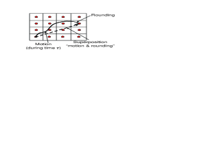
a) b)

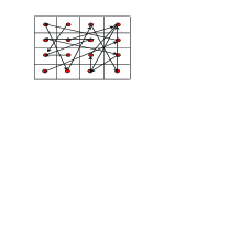
Figure 2: Motion, rounding and “motion with rounding” for a dynamical system (a), and the universal result of motion with rounding: a random dynamical system (b).

After rounding, some unexpected properties of dynamics appear. For example, even for transitive systems with strong mixing significant part of points of the $\varepsilon$-net becomes transient after rounding. Initially, attractor of such a continuous system is the whole phase space, but after rounding attractor of discrete dynamical system on the $\varepsilon$-net includes, roughly speaking, a half of its points (or, more precisely, the expectation of the number of transient points is $m({\rm e}-1)/{\rm e}$, where $m$ is number of points, ${\rm e}=2.7...$). In some circumstances, complicated dynamics has a tendency to collapse to trivial and degenerate behaviour as a result of discretizations Diamond . For systems without conservation of volume, the number of periodic points after discretization is linked to the dimension of the attractor $d$. The simple estimates based on the random map analysis, and numerical experiments with chaotic attractors give $\sim\varepsilon^{-d}$ for the number of periodic points, and $\sim\varepsilon^{-d/2}$ for the scale of the expected period GrebYor ; Hoower . The first of them is just the number of points in $\varepsilon$-net in $d$-dimensional compact, the second becomes clear after the following remark. Let us imagine a random walk in a finite set with $m$ elements (a $\varepsilon$-net). When the length of the trajectory is of order $\sqrt{m}$ then the next step returns the point to the trajectory with probability $\sim 1/\sqrt{m}$, and a loop appears with expected period $\sim\sqrt{m}$ (a half of the trajectory length). After $\sim\sqrt{m}$ steps the probability of a loop appearance is near $1$, hence, for the whole system the expected period is $\sim\sqrt{m}\sim\varepsilon^{-d/2}$.

It is easy to demonstrate the difference between coarse-graining by fattening and coarse-graining by rounding. Let us consider a trivial dynamics on a connected phase space: let the shift in time be identical transformation. For coarse-graining by fattening the $\varepsilon$-motion of any point tends to cover the whole phase space for any positive $\varepsilon$ and time $t\rightarrow\infty$: periodical $\varepsilon$-fattening with trivial dynamics transforms, after time $n\tau$, a point into the sum of $n$ $\varepsilon$-balls. For coarse-graining by rounding this trivial dynamical system generates the same trivial dynamical system on $\varepsilon$-net: nothing moves.

Coarse-graining by small noise seems to be very natural. We add small random term to the right hand side of differential equations that describe dynamics. Instead of the Liouville equation for probability density the Fokker–Planck equation appears. There is no fundamental difference between various types of coarse-graining, and the coarse-graining by $\varepsilon$-fattening includes major results about the coarse-graining by small noise that are insensitive to most details of noise distribution. But the knowledge of noise distribution gives us additional tools. The action functional is such a tool for the description of fluctuations [52] . Let $X^{\varepsilon}(t)$ be a random process “dynamics with $\varepsilon$-small fluctuation” on the time interval $[0,T]$. It is possible to introduce such a functional ${\bf S}[\varphi]$ on functions $x=\varphi(t)$ ($t\in[0,T]$) that for sufficiently small $\varepsilon,\delta>0$

$${\bf P}\{\|X^{\varepsilon}-\varphi\|<\delta\}\approx\exp(-{\bf S}[\varphi]/{\varepsilon}^{2}).$$

Action functional is constructed for various types of random perturbations [52] . Introduction to the general theory of random dynamical systems with invariant measure is presented in LArn .

In following sections, we consider two types of coarse-graining: the Ehrenfests’ coarse-graining and its extension to a general principle of non-equilibrium thermodynamics, and the coarse-graining based on the uncertainty of dynamical models and $\varepsilon$-motions.

2 The Ehrenfests’ Coarse-graining

2.1 Kinetic equation and entropy

Entropy conservation in systems with conservation of phase volume

The Erenfest’s coarse-graining was originally defined for conservative systems. Usually, Hamiltonian systems are considered as conservative ones, but in all constructions only one property of Hamiltonian systems is used, namely, conservation of the phase volume $\mathrm{d}\Gamma$ (the Liouville theorem). Let $X$ be phase space, $v(x)$ be a vector field, $\mathrm{d}\Gamma=\mathrm{d}^{n}x$ be the differential of phase volume. The flow,

$${\mathrm{d}x\over\mathrm{d}t}=v(x),$$ (1)

conserves the phase volume, if ${\rm div}v(x)=0$. The continuity equation,

$$\frac{\partial f}{\partial t}=-\sum_{i}\frac{\partial(fv_{i}(x))}{\partial x_{i}},$$ (2)

describes the induced dynamics of the probability density $f(x,t)$ on phase space. For incompressible flow (conservation of volume), the continuity equation can be rewritten in the form

$$\frac{\partial f}{\partial t}=-\sum_{i}v_{i}(x)\frac{\partial f}{\partial x_{i}}.$$ (3)

This means that the probability density is constant along the flow: $f(x,t+\mathrm{d}t)=f(x-v(x)\mathrm{d}t,t)$. Hence, for any continuous function $h(f)$ the integral

$$H(f)=\int_{X}h(f(x))\,\mathrm{d}\Gamma(x)$$ (4)

does not change in time, provided the probability density satisfies the continuity equation (2) and the flow $v(x)$ conserves the phase volume. For $h(f)=-f\ln f$ integral (4) gives the classical Boltzmann–Gibbs–Shannon (BGS) entropy functional:

$$S(f)=-\int_{X}f(x)\ln(f(x))\,\mathrm{d}\Gamma(x).$$ (5)

For flows with conservation of volume, entropy is conserved: $\mathrm{d}S/\mathrm{d}t\equiv 0$ .

Kullback entropy conservation in systems with regular invariant distribution

Suppose the phase volume is not invariant with respect to flow (1), but a regular invariant density $f^{*}(x)$ (equilibrium) exists:

$$\sum_{i}\frac{\partial(f^{*}(x)v_{i}(x))}{\partial x_{i}}=0.$$ (6)

In this case, instead of an invariant phase volume $\mathrm{d}\Gamma$, we have an invariant volume $f^{*}(x)\,\mathrm{d}\Gamma$. We can use (6) instead of the incompressibility condition and rewrite (2):

$$\frac{\partial(f(x,t)/f^{*}(x))}{\partial t}=-\sum_{i}v_{i}(x)\frac{\partial(f(x,t)/f^{*}(x))}{\partial x_{i}}.$$ (7)

The function $f(x,t)/f^{*}(x)$ is constant along the flow, the measure $f^{*}(x)\,\mathrm{d}\Gamma(x)$ is invariant, hence, for any continuous function $h(f)$ integral

$$H(f)=\int_{X}h(f(x,t)/f^{*}(x))f^{*}(x)\,\mathrm{d}\Gamma(x)$$ (8)

does not change in time, if the probability density satisfies the continuity equation. For $h(f)=-f\ln f$ integral (8) gives the Kullback entropy functional Kull :

$$S_{K}(f)=-\int_{X}f(x)\ln\left(\frac{f(x)}{f^{*}(x)}\right)\,\mathrm{d}\Gamma(x).$$ (9)

This situation does not differ significantly from the entropy conservation in systems with conservation of volume. It is just a kind of change of variables.

General entropy production formula

Let us consider the general case without assumptions about phase volume invariance and existence of a regular invariant density (6). In this case, let a probability density $f(x,t)$ be a solution of the continuity equation (2). For the BGS entropy functional (5)

$$\frac{\mathrm{d}S(f)}{\mathrm{d}t}=\int_{X}f(x,t){\rm div}v(x)\,\mathrm{d}\Gamma(x),$$ (10)

if the left hand side exists. This entropy production formula can be easily proven for small phase drops with constant density, and then for finite sums of such distributions with positive coefficients. After that, we obtain formula (10) by limit transition.

For a regular invariant density $f^{*}(x)$ (equilibrium) entropy $S(f^{*})$ exists, and for this distribution $\mathrm{d}S(f)/\mathrm{d}t=0$, hence,

$$\int_{X}f^{*}(x){\rm div}v(x)\,\mathrm{d}\Gamma(x)=0.$$ (11)

Entropy production in systems without regular equilibrium

If there is no regular equilibrium (6), then the entropy behaviour changes drastically. If volume of phase drops tends to zero, then the BGS entropy (5) and any Kullback entropy (9) goes to minus infinity. The simplest example clarifies the situation. Let all the solutions converge to unique exponentially stable fixed point $x=0$. In linear approximation $\mathrm{d}x/\mathrm{d}t=Ax$ and $S(t)=S(0)+t\,{\rm tr}A.$ Entropy decreases linearly in time with the rate ${\rm tr}A$ (${\rm tr}A={\rm div}v(x)$, ${\rm tr}A<0$), time derivative of entropy is ${\rm tr}A$ and does not change in time, and the probability distribution goes to the $\delta$-function $\delta(x)$. Entropy of this distribution does not exist (it is “minus infinity”), and it has no limit when $f(x,t)\rightarrow\delta(x)$.

Nevertheless, time derivative of entropy is well defined and constant, it is ${\rm tr}A$. For more complicated singular limit distributions the essence remains the same: according to (10) time derivative of entropy tends to the average value of ${\rm div}v(x)$ in this limit distribution, and entropy goes linearly to minus infinity (if this average in not zero, of course). The order in the system increases. This behaviour could sometimes be interpreted as follows: the system is open and produces entropy in its surrounding even in a steady–state. Much more details are in review Ruelle .

Starting point: a kinetic equation

For the formalization of the Ehrenfests’ idea of coarse-graining, we start from a formal kinetic equation

$$\frac{\mathrm{d}f}{\mathrm{d}t}=J(f)$$ (12)

with a concave entropy functional $S(f)$ that does not increase in time. This equation is defined in a convex subset $U$ of a vector space $E$.

Let us specify some notations: $E^{T}$ is the adjoint to the $E$ space. Adjoint spaces and operators will be indicated by ^T, whereas the notation ^∗ is earmarked for equilibria and quasi-equilibria.

We recall that, for an operator $A:E_{1}\to E_{2}$, the adjoint operator, $A^{T}:E_{1}^{T}\to E_{2}^{T}$ is defined by the following relation: for any $l\in E_{2}^{T}$ and $\varphi\in E_{1}$, $l(A\varphi)=(A^{T}l)(\varphi)$.

Next, $D_{f}S(f)\in E^{T}$ is the differential of the functional $S(f)$, $D^{2}_{f}S(f)$ is the second differential of the functional $S(f)$. The quadratic functional $D^{2}_{f}S(f)(\varphi,\varphi)$ on $E$ is defined by the Taylor formula,

$$S(f+\varphi)=S(f)+D_{f}S(f)(\varphi)+\frac{1}{2}D_{f}^{2}S(f)(\varphi,\varphi)+o(\|\varphi\|^{2}).$$ (13)

We keep the same notation for the corresponding symmetric bilinear form, $D_{f}^{2}S(f)(\varphi,\psi)$, and also for the linear operator, $D_{f}^{2}S(f):E\to E^{T}$, defined by the formula $(D_{f}^{2}S(f)\varphi)(\psi)=D_{f}^{2}S(f)(\varphi,\psi)$. In this formula, on the left hand side $D_{f}^{2}S(f)$ is the operator, on the right hand side it is the bilinear form. Operator $D_{f}^{2}S(f)$ is symmetric on $E$, $D_{f}^{2}S(f)^{T}=D_{f}^{2}S(f)$.

In finite dimensions the functional $D_{f}S(f)$ can be presented simply as a row vector of partial derivatives of $S$, and the operator $D_{f}^{2}S(f)$ is a matrix of second partial derivatives. For infinite–dimensional spaces some complications exist because $S(f)$ is defined only for classical densities and not for all distributions. In this paper we do not pay attention to these details.

We assume strict concavity of $S$, $D_{f}^{2}S(f)(\varphi,\varphi)<0$ if $\varphi\neq 0$. This means that for any $f$ the positive definite quadratic form $-D_{f}^{2}S(f)(\varphi,\varphi)$ defines a scalar product

$$\langle\varphi,\psi\rangle_{f}=-(D_{f}^{2}S)(\varphi,\psi).$$ (14)

This entropic scalar product is an important part of thermodynamic formalism. For the BGS entropy (5) as well as for the Kullback entropy (9)

$$\langle\varphi,\psi\rangle_{f}=\int\frac{\varphi(x)\psi(x)}{f(x)}\,\mathrm{d}x.$$ (15)

The most important assumption about kinetic equation (12) is: entropy does not decrease in time:

$$\frac{\mathrm{d}S}{\mathrm{d}t}=(D_{f}S(f))(J(f))\geq 0.$$ (16)

A particular case of this assumption is: the system (12) is conservative and entropy is constant. The main example of such conservative equations is the Liouville equation with linear vector field $J(f)=-Lf=\{H,f\}$, where $\{H,f\}$ is the Poisson bracket with Hamiltonian $H$.

For the following consideration of the Ehrenfests’ coarse-graining the underlying mechanical motion is not crucial, and it is possible to start from the formal kinetic equation (12) without any mechanical interpretation of vectors $f$. We develop below the coarse-graining procedure for general kinetic equation (12) with non-decreasing entropy (16). After coarse-graining the entropy production increases: conservative systems become dissipative ones, and dissipative systems become “more dissipative.”

2.2 Conditional equilibrium instead of averaging in cells

Microdescription, macrodescription and quasi-equilibrium state

Averaging in cells is a particular case of entropy maximization. Let the phase space be divided into cells. For the $i$th cell the population $M_{i}$ is

$$M_{i}=m_{i}(f)=\int_{{\rm cell}_{i}}f(x)\,\mathrm{d}\Gamma(x).$$

The averaging in cells for a given vector of populations $M=(M_{i})$ produces the solution of the optimization problem for the BGS entropy:

$$S(f)\to\max,\ m(f)=M,$$ (17)

where $m(f)$ is vector $(m_{i}(f))$. The maximizer is a function $f^{*}_{M}(x)$ defined by the vector of averages $M$.

This operation has a well-known generalization. In the more general statement, vector $f$ is a microscopic description of the system, vector $M$ gives a macroscopic description, and a linear operator $m$ transforms a microscopic description into a macroscopic one: $M=m(f)$. The standard example is the transformation of the microscopic density into the hydrodynamic fields (density–velocity–kinetic temperature) with local Maxwellian distributions as entropy maximizers (see, for example, GorKar ).

Figure 3: Relations between a microscopic state $f$, a corresponding macroscopic state $M=m(f)$, and a quasi-equilibrium state $f^{*}_{M}$.

For any macroscopic description $M$, let us define the correspondent $f^{*}_{M}$ as a solution to optimization problem (17) with an appropriate entropy functional $S(f)$ (Fig. 3). This $f^{*}_{M}$ has many names in the literature: MaxEnt distribution, reference distribution (reference of the macroscopic description to the microscopic one), generalized canonical ensemble, conditional equilibrium, or quasi-equilibrium. We shall use here the last term.

The quasi-equilibrium distribution $f^{*}_{M}$ satisfies the obvious, but important identity of self-consistency:

$$m(f^{*}_{M})=M,$$ (18)

or in differential form

$$m(D_{M}f^{*}_{M})=1,\;{\rm i.e.}\;m((D_{M}f^{*}_{M})a)\equiv a.$$ (19)

The last identity means that the infinitesimal change in $M$ calculated through differential of the quasi-equilibrium distribution $f^{*}_{M}$ is simply the infinitesimal change in $M$. For the second differential we obtain

$$m(D^{2}_{M}f^{*}_{M})=0,\;{\rm i.e.}\;m((D^{2}_{M}f^{*}_{M})(a,b))\equiv 0.$$ (20)

Following GorKar let us mention that most of the works on nonequilibrium thermodynamics deal with quasi-equilibrium approximations and corrections to them, or with applications of these approximations (with or without corrections). This viewpoint is not the only possible but it proves very efficient for the construction of a variety of useful models, approximations and equations, as well as methods to solve them.

From time to time it is discussed in the literature, who was the first to introduce the quasi-equilibrium approximations, and how to interpret them. At least a part of the discussion is due to a different role the quasi-equilibrium plays in the entropy-conserving and in the dissipative dynamics. The very first use of the entropy maximization dates back to the classical work of G. W. Gibbs Gibb , but it was first claimed for a principle of informational statistical thermodynamics by E. T. Jaynes Janes1 . Probably, the first explicit and systematic use of quasiequilibria on the way from entropy-conserving dynamics to dissipative kinetics was undertaken by D. N. Zubarev. Recent detailed exposition of his approach is given in Zubarev .

For dissipative systems, the use of the quasi-equilibrium to reduce description can be traced to the works of H. Grad on the Boltzmann equation Grad . A review of the informational statistical thermodynamics was presented in Garsia1 . The connection between entropy maximization and (nonlinear) Onsager relations was also studied Nett ; Orlov84 . Our viewpoint was influenced by the papers by L. I. Rozonoer and co-workers, in particular, KoRoz ; Ko ; Roz . A detailed exposition of the quasi-equilibrium approximation for Markov chains is given in the book G1 (Chap. 3, Quasi-equilibrium and entropy maximum, pp. 92-122), and for the BBGKY hierarchy in the paper Kark .

The maximum entropy principle was applied to the description of the universal dependence of the three-particle distribution function $F_{3}$ on the two-particle distribution function $F_{2}$ in classical systems with binary interactions BGKTMF . For a discussion of the quasi-equilibrium moment closure hierarchies for the Boltzmann equation Ko see the papers MBCh ; MBChLANL ; Lever . A very general discussion of the maximum entropy principle with applications to dissipative kinetics is given in the review Bal . Recently, the quasi-equilibrium approximation with some further correction was applied to the description of rheology of polymer solutions IKOePhA02 ; IKOePhA03 and of ferrofluids IlKr ; IKar2 . Quasi-equilibrium approximations for quantum systems in the Wigner representation WIG ; CAL was discussed very recently Degon .

We shall now introduce the quasi-equilibrium approximation in the most general setting. The coarse-graining procedure will be developed after that as a method for enhancement of the quasi-equilibrium approximation GKIOeNONNEWT2001 .

Quasi-equilibrium manifold, projector and approximation

A quasi-equilibrium manifold is a set of quasi-equilibrium states $f^{*}_{M}$ parameterized by macroscopic variables $M$. For microscopic states $f$ the correspondent quasi-equilibrium states are defined as $f^{*}_{m(f)}$. Relations between $f$, $M$, $f^{*}_{M}$, and $f^{*}_{m(f)}$ are presented in Fig. 3.

A quasi-equilibrium approximation for the kinetic equation (12) is an equation for $M(t)$:

$$\frac{\mathrm{d}M}{\mathrm{d}t}=m(J(f^{*}_{M})).$$ (21)

To define $\dot{M}$ in the quasi-equilibrium approximation for given $M$, we find the correspondent quasi-equilibrium state $f^{*}_{M}$ and the time derivative of $f$ in this state $J(f^{*}_{M})$, and then return to the macroscopic variables by the operator $m$. If $M(t)$ satisfies (21) then $f^{*}_{M(t)}$ satisfies the following equation

$$\frac{\mathrm{d}f^{*}_{M}}{\mathrm{d}t}=(D_{M}f^{*}_{M})\left(\frac{\mathrm{d}M}{\mathrm{d}t}\right)=(D_{M}f^{*}_{M})(m(J(f^{*}_{M}))).$$ (22)

The right hand side of (22) is the projection of vector field $J(f)$ onto the tangent space of the quasi-equilibrium manifold at the point $f=f^{*}_{M}$. After calculating the differential $D_{M}f^{*}_{M}$ from the definition of quasi-equilibrium (17), we obtain ${\mathrm{d}f^{*}_{M}}/{\mathrm{d}t}=\pi_{f^{*}_{M}}J(f^{*}_{M})$, where $\pi_{f^{*}_{M}}$ is the quasi-equilibrium projector:

$$\pi_{f^{*}_{M}}=\left(D_{M}f^{*}_{M}\right)m=\left(D_{f}^{2}S\right)_{f^{*}_{M}}^{-1}m^{T}\left(m\left(D_{f}^{2}S\right)_{f^{*}_{M}}^{-1}m^{T}\right)^{-1}m.$$ (23)

It is straightforward to check the equality $\pi_{f^{*}_{M}}^{2}=\pi_{f^{*}_{M}}$, and the self-adjointness of $\pi_{f^{*}_{M}}$ with respect to entropic scalar product (14). In this scalar product, the quasi-equilibrium projector is the orthogonal projector onto the tangent space to the quasi-equilibrium manifold.

Figure 4: Quasi-equilibrium manifold $\Omega$, tangent space $T_{f^{*}_{M}}\Omega$, quasi-equilibrium projector $\pi_{f^{*}_{M}}$, and defect of invariance, $\Delta_{f^{*}_{M}}=J-\pi_{f^{*}_{M}}(J)$.

The quasi-equilibrium projector for a quasi-equilibrium approximation was first constructed by B. Robertson Robertson .

Thus, we have introduced the basic constructions: quasi-equilibrium manifold, entropic scalar product, and quasi-equilibrium projector (Fig. 4).

Preservation of dissipation

For the quasi-equilibrium approximation the entropy is $S(M)=S(f^{*}_{M})$. For this entropy,

$$\frac{\mathrm{d}S(M)}{\mathrm{d}t}=\left(\frac{\mathrm{d}S(f)}{\mathrm{d}t}\right)_{f=f^{*}_{M}},$$ (24)

Here, on the left hand side stands the macroscopic entropy production for the quasi-equilibrium approximation (21), and the right hand side is the microscopic entropy production calculated for the initial kinetic equation (12). This equality implies preservation of the type of dynamics G1 ; Ocherki :

• If for the initial kinetics (12) the dissipativity inequality (16) holds then the same inequality is true for the quasi-equilibrium approximation (21);

• If the initial kinetics (12) is conservative then the quasi-equilibrium approximation (21) is conservative also.

For example, let the initial kinetic equation be the Liouville equation for a system of many identical particles with binary interaction. If we choose as macroscopic variables the one-particle distribution function, then the quasi-equilibrium approximation is the Vlasov equation. If we choose as macroscopic variables the hydrodynamic fields, then the quasi-equilibrium approximation is the compressible Euler equation with self–interaction of liquid. Both of these equations are conservative and turn out to be even Hamiltonian systems Morrison .

Measurement of accuracy

Accuracy of the quasi-equilibrium approximation near a given $M$ can be measured by the defect of invariance (Fig. 4):

$$\Delta_{f^{*}_{M}}=J(f^{*}_{M})-\pi_{f^{*}_{M}}J(f^{*}_{M}).$$ (25)

A dimensionless criterion of accuracy is the ratio $\|\Delta_{f^{*}_{M}}\|/\|J(f^{*}_{M})\|$ (a “sine” of the angle between $J$ and tangent space). If $\Delta_{f^{*}_{M}}\equiv 0$ then the quasi-equilibrium manifold is an invariant manifold, and the quasi-equilibrium approximation is exact. In applications, the quasi-equilibrium approximation is usually not exact.

The Gibbs entropy and the Boltzmann entropy

For analysis of micro-macro relations some authors LebBloEnt ; Bentr call entropy $S(f)$ the Gibbs entropy, and introduce a notion of the Boltzmann entropy. Boltzmann defined the entropy of a macroscopic system in a macrostate $M$ as the $\log$ of the volume of phase space (number of microstates) corresponding to $M$. In the proposed level of generality G1 ; Ocherki , the Boltzmann entropy of the state $f$ can be defined as $S_{\rm B}(f)=S(f^{*}_{m(f)})$. It is entropy of the projection of $f$ onto quasi-equilibrium manifold (the “shadow” entropy). For conservative systems the Gibbs entropy is constant, but the Boltzmann entropy increases Ocherki (during some time, at least) for motions that start on the quasi-equilibrium manifold, but not belong to this manifold.

These notions of the Gibbs or Boltzmann entropy are related to micro-macro transition and may be applied to any convex entropy functional, not the BGS entropy (5) only. This may cause some terminological problems (we hope, not here), and it may be better just to call $S(f^{*}_{m(f)})$ the macroscopic entropy.

Invariance equation and the Chapman–Enskog expansion

The first method for improvement of the quasi-equilibrium approximation was the Chapman–Enskog method for the Boltzmann equation Chapman . It uses the explicit structure of singularly perturbed systems. Many other methods were invented later, and not all of them use this explicit structure (see, for example review in GorKar ). Here we develop the Chapman–Enskog method for one important class of model equations that were invented to substitute the Boltzmann equation and other more complicated systems when we don’t know the details of microscopic kinetics. It includes the well-known Bhatnagar–Gross–Krook (BGK) kinetic equation BGK , as well as wide class of generalized model equations GKMod .

As a starting point we take a formal kinetic equation with a small parameter $\epsilon$

$$\frac{\mathrm{d}f}{\mathrm{d}t}=J(f)=F(f)+\frac{1}{\epsilon}(f^{*}_{m(f)}-f).$$ (26)

The term $(f^{*}_{m(f)}-f)$ is non-linear because nonlinear dependency $f^{*}_{m(f)}$ on $m(f)$.

We would like to find a reduced description valid for macroscopic variables $M$. It means, at least, that we are looking for an invariant manifold parameterized by $M$, $f=f_{M}$, that satisfies the invariance equation:

$$(D_{M}f_{M})(m(J(f_{M})))=J(f_{M}).$$ (27)

The invariance equation means that the time derivative of $f$ calculated through the time derivative of $M$ ($\dot{M}=m(J(f_{M}))$) by the chain rule coincides with the true time derivative $J(f)$. This is the central equation for the model reduction theory and applications. First general results about existence and regularity of solutions to that equation were obtained by Lyapunov Lya (see review in CMIM ; GorKar ). For kinetic equation (26) the invariance equation has a form

$$(D_{M}f_{M})(m(F(f_{M})))=F(f_{M})+\frac{1}{\epsilon}(f^{*}_{M}-f_{M}),$$ (28)

because the self-consistency identity (18).

Due to presence of small parameter $\epsilon$ in $J(f)$, the zero approximation is obviously the quasi-equilibrium approximation: $f^{(0)}_{M}=f^{*}_{M}$. Let us look for $f_{M}$ in the form of power series: $f_{M}=f^{(0)}_{M}+{\epsilon}f^{(1)}_{M}+\ldots$; $m(f^{(k)}_{M})=0$ for $k\geq 1$. From (28) we immediately find:

$$f^{(1)}_{M}=F(f^{(0)}_{M})-(D_{M}f^{(0)}_{M})(m(F(f^{(0)}_{M})))=\Delta_{f^{*}_{M}}.$$ (29)

It is very natural that the first term of the Chapman–Enskog expansion for model equations (26) is just the defect of invariance for the quasi-equilibrium approximation. Calculation of the following terms is also straightforward.

The correspondent first–order in $\epsilon$ approximation for the macroscopic equations is:

$$\frac{\mathrm{d}M}{\mathrm{d}t}=m(F(f^{*}_{M}))+\epsilon m((D_{f}F(f))_{f^{*}_{M}}\Delta_{f^{*}_{M}}).$$ (30)

We should remind that $m(\Delta_{f^{*}_{M}})=0$. The last term in (28) vanishes in macroscopic projection for all orders.

The typical situation for the model equations (26) is: the vector field $F(f)$ is conservative, $(D_{f}S(f))F(f)=0$. In that case, the first term $m(F(f^{*}_{M}))$ also conserves the correspondent Boltzmann (i.e. macroscopic, but not obligatory BGS) entropy $S(f^{*}_{M})$. But the straightforward calculation of the Boltzmann entropy $S(f^{*}_{M})$ production for the first-order Chapman–Enskog term in equation (30) gives us for conservative $F(f)$:

$$\frac{\mathrm{d}S(M)}{\mathrm{d}t}=\epsilon\langle\Delta_{f^{*}_{M}},\Delta_{f^{*}_{M}}\rangle_{f^{*}_{M}}\geq 0.$$ (31)

where $\langle\bullet,\bullet\rangle_{f}$ is the entropic scalar product (14). The Boltzmann entropy production in the first Chapman–Enskog approximation is zero if and only if $\Delta_{f^{*}_{M}}=0$, i.e. if at point $M$ the quasi-equilibrium manifold is locally invariant.

To prove (31) we differentiate the conservativity identity:

$$(D_{f}S(f))F(f)\equiv 0$$ (32)

$$(D^{2}_{f}S(F))(F(f),a)+(D_{f}S(f))((D_{f}F(f))a)\equiv 0$$

$$(D_{f}S(f))((D_{f}F(f))a)\equiv\langle F(f),a\rangle_{f},$$

use the last equality in the expression of the entropy production, and take into account that the quasi-equilibrium projector is orthogonal, hence

$$\langle F({f^{*}_{M}}),\Delta_{f^{*}_{M}}\rangle_{f^{*}_{M}}=\langle\Delta_{f^{*}_{M}},\Delta_{f^{*}_{M}}\rangle_{f^{*}_{M}}.$$

Below we apply the Chapman–Enskog method to the analysis of filtered BGK equation.

2.3 The Ehrenfests’ Chain, Macroscopic Equations and Entropy production

The Ehrenfests’ Chain and entropy growth

Let $\Theta_{t}$ be the time shift transformation for the initial kinetic equation (12):

$$\Theta_{t}(f(0))=f(t).$$

The Ehrenfests’ chain (Fig. 5) is defined for a given macroscopic variables $M=m(f)$ and a fixed time of coarse-graining $\tau$. It is a chain of quasi-equilibrium states $f_{0},f_{1},\ldots$:

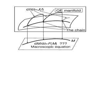
Figure 5: The Ehrenfests’ chain.

$$f_{i+1}=f^{*}_{m(\Theta_{\tau}(f_{i}))}.$$ (33)

To get the next point of the chain, $f_{i+1}$, we take $f_{i}$, move it by the time shift $\Theta_{\tau}$, calculate the corresponding macroscopic state $M_{i+1}=m(\Theta_{\tau}(f_{i}))$, and find the quasi-equilibrium state $f^{*}_{M_{i+1}}=f_{i+1}$.

If the point $\Theta_{\tau}(f_{i})$ is not a quasi-equilibrium state, then $S(\Theta_{\tau}(f_{i}))<S(f^{*}_{m(\Theta_{\tau}(f_{i}))})$ because of quasi-equilibrium definition (17) and strict concavity of entropy. Hence, if the motion between $f_{i}$ and $\Theta_{\tau}(f_{i})$ does not belong to the quasi-equilibrium manifold, then $S(f_{i+1})>S(f_{i})$, entropy in the Ehrenfests’ chain grows. The entropy gain consists of two parts: the gain in the motion (from $f_{i}$ to $\Theta_{\tau}(f_{i})$), and the gain in the projection (from $\Theta_{\tau}(f_{i})$ to $f_{i+1}=f^{*}_{m(\Theta_{\tau}(f_{i}))}$). Both parts are non-negative. For conservative systems the first part is zero. The second part is strictly positive if the motion leaves the quasi-equilibrium manifold. Hence, we observe some sort of duality between entropy production in the Ehrenfests’ chain and invariance of the quasi-equilibrium manifold. The motions that build the Ehrenfests’ chain restart periodically from the quasi-equilibrium manifold and the entropy growth along this chain is similar to the Boltzmann entropy growth in the Chapman–Enskog approximation, and that similarity is very deep, as the exact formulas show below.

The natural projector and macroscopic dynamics

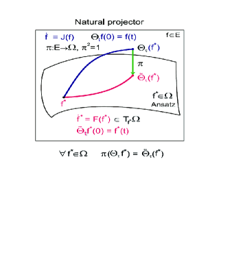
Figure 6: Projection of segments of trajectories: The microscopic motion above the manifold $\Omega$ and the macroscopic motion on this manifold. If these motions begin in the same point on $\Omega$, then, after time $\tau$, projection of the microscopic state onto $\Omega$ should coincide with the result of the macroscopic motion on $\Omega$. For quasi-equilibrium $\Omega$, projector $\pi:E\rightarrow\Omega$ acts as $\pi(f)=f^{*}_{m(f)}$.

How to use the Ehrenfests’ chains? First of all, we can try to define the macroscopic kinetic equations for $M(t)$ by the requirement that for any initial point of the chain $f_{0}$ the solution of these macroscopic equations with initial conditions $M(0)=m(f_{0})$ goes through all the points $m(f_{i})$: $M(n\tau)=m(f_{n})$ ($n=1,2,\ldots$) (Fig. 5) GKIOeNONNEWT2001 (see also GorKar ). Another way is an “equation–free approach” KevFree to the direct computation of the Ehrenfests’ chain with a combination of microscopic simulation and macroscopic stepping.

For the definition of the macroscopic equations only the first link of the Ehrenfests’ chain is necessary. In general form, for an ansatz manifold $\Omega$, projector $\pi:U\rightarrow\Omega$ of the vicinity of $\Omega$ onto $\Omega$, phase flow of the initial kinetic equation $\Theta_{t}$, and macroscopic phase flow $\tilde{\Theta}_{t}$ on $\Omega$ the matching condition is (Fig. 6):

$$\pi(\Theta_{\tau}(f))=\tilde{\Theta}_{\tau}(f)\;\mbox{for any}\;f\in\Omega.$$ (34)

We call this projector of the flow $\Theta$ onto an ansatz manifold $\Omega$ by fragments of trajectories of given duration $\tau$ the natural projector in order to distinguish it from the standard infinitesimal projector of vector fields on tangent spaces.

Let us look for the macroscopic equations of the form

$$\frac{\mathrm{d}M}{\mathrm{d}t}=\Psi(M)$$ (35)

with the phase flow $\Phi_{t}$: $M(t)=\Phi_{t}M(0)$. For the quasi-equilibrium manifold and projector the matching condition (34) gives

$$m(\Theta_{\tau}(f^{*}_{M}))=\Phi_{\tau}(M)\;\mbox{for any macroscopic state}\;M.$$ (36)

This condition is the equation for the macroscopic vector field $\Psi(M)$. The solution of this equation is a function of $\tau$: $\Psi=\Psi(M,\tau)$. For sufficiently smooth microscopic vector field $J(f)$ and entropy $S(f)$ it is easy to find the Taylor expansion of $\Psi(M,\tau)$ in powers of $\tau$. It is a straightforward exercise in differential calculus. Let us find the first two terms: $\Psi(M,\tau)=\Psi_{0}(M)+\tau\Psi_{1}(M)+o(\tau)$. Up to the second order in $\tau$ the matching condition (36) is

$$m(J(f^{*}_{M}))\tau+m((D_{f}J(f))_{f=f^{*}_{M}}(J(f^{*}_{M})))\frac{\tau^{2}}{2}$$

$$=\Psi_{0}(M)\tau+\Psi_{1}(M)\tau^{2}+(D_{M}\Psi_{0}(M))(\Psi_{0}(M))\frac{\tau^{2}}{2}.$$ (37)

From this condition immediately follows:

$$\Psi_{0}(M) = m(J(f^{*}_{M}));$$ (38)

$$\Psi_{1}(M) = \frac{1}{2}m[(D_{f}J(f))_{f=f^{*}_{M}}(J(f^{*}_{M}))-(D_{M}J(f^{*}_{M}))(m(J(f^{*}_{M})))]$$

$$= m((D_{f}J(f))_{f=f^{*}_{M}}\Delta_{f^{*}_{M}})$$

where $\Delta_{f^{*}_{M}}$ is the defect of invariance (25). The macroscopic equation in the first approximation is:

$$\frac{\mathrm{d}M}{\mathrm{d}t}=m(J(f^{*}_{M}))+\frac{\tau}{2}m((D_{f}J(f))_{f=f^{*}_{M}}\Delta_{f^{*}_{M}}).$$ (39)

It is exactly the first Chapman–Enskog approximation (30) for the model kinetics (26) with $\varepsilon={\tau}/{2}$. The first term $m(J(f^{*}_{M}))$ gives the quasi-equilibrium approximation, the second term increases dissipation. The formula for entropy production follows from (39) GKOeTPRE2001 . If the initial microscopic kinetic (12) is conservative, then for macroscopic equation (39) we obtain as for the Chapman–Enskog approximation:

$$\frac{\mathrm{d}S(M)}{\mathrm{d}t}=\frac{\tau}{2}\langle\Delta_{f^{*}_{M}},\Delta_{f^{*}_{M}}\rangle_{f^{*}_{M}},$$ (40)

where $\langle\bullet,\bullet\rangle_{f}$ is the entropic scalar product (14). From this formula we see again a duality between the invariance of the quasi-equilibrium manifold and the dissipativity: entropy production is proportional to the square of the defect of invariance of the quasi-equilibrium manifold.

For linear microscopic equations ($J(f)=Lf$) the form of the macroscopic equations is

$$\frac{\mathrm{d}M}{\mathrm{d}t}=mL\left[1+\frac{\tau}{2}(1-\pi_{f^{*}_{M}})L\right]f^{*}_{M},$$ (41)

where $\pi_{f^{*}_{M}}$ is the quasi-equilibrium projector (23).

The Navier–Stokes equation from the free flight dynamics

The free flight equation describes dynamics of one-particle distribution function $f(\mbox{\boldmath$x$},\mbox{\boldmath$v$})$ due to free flight:

$$\frac{\partial f(\mbox{\boldmath$x$},\mbox{\boldmath$v$},t)}{\partial t}=-\sum_{i}v_{i}\frac{\partial f(\mbox{\boldmath$x$},\mbox{\boldmath$v$},t)}{\partial x_{i}}.$$ (42)

The difference from the continuity equation (2) is that there is no velocity field $\mbox{\boldmath$v$}(\mbox{\boldmath$x$})$, but the velocity vector $v$ is an independent variable. Equation (42) is conservative and has an explicit general solution

$$f(\mbox{\boldmath$x$},\mbox{\boldmath$v$},t)=f_{0}(\mbox{\boldmath$x$}-\mbox{\boldmath$v$}t,\mbox{\boldmath$v$}).$$ (43)

The coarse-graining procedure for (42) serves for modeling kinetics with an unknown dissipative term $I(f)$

$$\frac{\partial f(\mbox{\boldmath$x$},\mbox{\boldmath$v$},t)}{\partial t}=-\sum_{i}v_{i}\frac{\partial f(\mbox{\boldmath$x$},\mbox{\boldmath$v$},t)}{\partial x_{i}}+I(f).$$ (44)

The Ehrenfests’ chain realizes a splitting method for (44): first, the free flight step during time $\tau$, than the complete relaxation to a quasi-equilibrium distribution due to dissipative term $I(f)$, then again the free flight, and so on. In this approximation the specific form of $I(f)$ is not in use, and the only parameter is time $\tau$. It is important that this hypothetical $I(f)$ preserves all the standard conservation laws (number of particles, momentum, and energy) and has no additional conservation laws: everything else relaxes. Following this assumption, the macroscopic variables are: $M_{0}=n(\mbox{\boldmath$x$},t)=\int f\mathrm{d}\mbox{\boldmath$v$}$, $M_{i}=nu_{i}=\int v_{i}f\mathrm{d}\mbox{\boldmath$v$}$ ($i=1,2,3$), $M_{4}=\frac{3nk_{\rm B}T}{m}+nu^{2}=\int v^{2}f\mathrm{d}\mbox{\boldmath$v$}$. The zero-order (quasi-equilibrium) approximation (21) gives the classical Euler equation for compressible non-isothermal gas. In the first approximation (39) we obtain the Navier–Stokes equations:

$${\partial n\over\partial t} = -\sum_{i}{\partial(nu_{i})\over\partial x_{i}},$$

$${\partial(nu_{k})\over\partial t} = -\sum_{i}{\partial(nu_{k}u_{i})\over\partial x_{i}}-\frac{1}{m}{\partial P\over\partial x_{k}}$$ (45)

$$+\underline{{\tau\over 2}\frac{1}{m}\sum_{i}{\partial\over\partial x_{i}}\left[P\left({\partial u_{k}\over\partial x_{i}}+{\partial u_{i}\over\partial x_{k}}-{2\over 3}\delta_{ki}{\rm div}u\right)\right]},$$

$${\partial\mathcal{E}\over\partial t} = -\sum_{i}{\partial(\mathcal{E}u_{i})\over\partial x_{i}}-\frac{1}{m}\sum_{i}{\partial(Pu_{i})\over\partial x_{i}}+\underline{\frac{\tau}{2}{5k_{\rm B}\over 2m^{2}}\sum_{i}{\partial\over\partial x_{i}}\left(P{\partial T\over\partial x_{i}}\right)},$$

where $P=nk_{\rm B}T$ is the ideal gas pressure, $\mathcal{E}=\frac{1}{2}\int v^{2}f\,\mathrm{d}\mbox{\boldmath$v$}=\frac{3nk_{\rm B}T}{2m}+\frac{n}{2}u^{2}$ is the energy density per unite mass ($P=\frac{2m}{3}\mathcal{E}-\frac{mn}{3}u^{2}$, $T=\frac{2m}{3nk_{\rm B}}\mathcal{E}-\frac{m}{3k_{\rm B}}u^{2}$), and the underlined terms are results of the coarse-graining additional to the quasi-equilibrium approximation.

The dynamic viscosity in (2.3) is $\mu=\frac{\tau}{2}nk_{\rm B}T$. It is useful to compare this formula to the mean–free–path theory that gives $\mu=\tau_{\rm col}nk_{\rm B}T=\tau_{\rm col}P$, where $\tau_{\rm col}$ is the collision time (the time for the mean–free–path). According to these formulas, we get the following interpretation of the coarse-graining time $\tau$ for this example: $\tau=2\tau_{\rm col}$.

The equations obtained (2.3) coincide with the first–order terms of the Chapman–Enskog expansion (30) applied to the BGK equations with $\tau_{\rm col}=\tau/2$ and meet the same problem: the Prandtl number (i.e., the dimensionless ratio of viscosity and thermal conductivity) is ${\rm Pr}=1$ instead of the value ${\rm Pr}=\frac{2}{3}$ verified by experiments with perfect gases and by more detailed theory Cercignani (recent discussion of this problem for the BGK equation with some ways for its solution is presented in Struch ).

In the next order in $\tau$ we obtain the stable post–Navier–Stokes equations instead of the unstable Burnett equations that appear in the Chapman–Enskog expansion GKOeTPRE2001 ; KTGOePhA2003 . Here we can see the difference between two approaches.

Persistence of invariance and mistake of differential pursuit

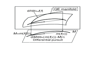
a) b)

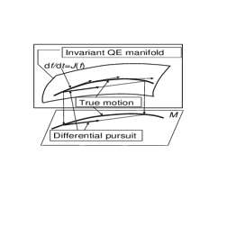
Figure 7: Differential pursuit of the projection point (a). The mistake of differential pursuit (b): invariant manifold should preserve its invariance, but it does not!

L.M. Lewis called a generalization of the Ehernfest’s approach a “unifying principle in statistical mechanics,” but he created other macroscopic equations: he produced the differential pursuit (Fig. 7a)

$$\frac{\mathrm{d}M}{\mathrm{d}t}=\frac{m(\Theta_{\tau}(f^{*}_{M}))-M}{\tau}$$ (46)

from the full matching condition (34). This means that the macroscopic motion was taken in the first-order Tailor approximation, while for the microscopic motion the complete shift in time (without the Taylor expansion) was used. The basic idea of this approach is a non-differential time separation: the infinitesimal shift in macroscopic time is always such a significant shift for microscopic time that no Taylor approximation for microscopic motion may be in use. This sort of non-standard analysis deserves serious attention, but its realization in the form of the differential pursuit (46) does not work properly in many cases. If the quasi-equilibrium manifold is invariant, then the quasi-equilibrium approximation is exact and the Ehrenfests’ chain (Fig. 5) just follows the quasi-equilibrium trajectory. But the differential pursuit does not follow the trajectory (Fig. 7b); this motion leaves the invariant quasi-equilibrium manifolds, and the differential pursuit does not approximate the Ehrenfests’ chain, even qualitatively.

Ehrenfests’ coarse-graining as a method for model reduction

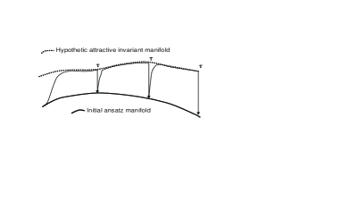
Figure 8: Natural projector and attractive invariant manifolds. For large $\tau$, the natural projector gives the approximation of projection of the genuine motion from the attractive invariant manifold onto the initial ansatz manifold $\Omega$.

The problem of model reduction in dissipative kinetics is recognized as a problem of time separation and construction of slow invariant manifolds. One obstacle on this way is that the slow invariant manifold is the thing that many people would like to find, but nobody knows exactly what it is. There is no conventional definition of slow invariant manifold without explicit small parameter that tends to zero. It seems now that the most reasonable way for such a definition is the analysis of induced dynamics of manifolds immersed into phase space. Fixed points of this dynamics are invariant manifolds, and asymptotically stable (stable and attracting) fixed points are slow invariant manifolds. This concept was explicitly developed very recently Shnol ; CMIM ; GorKar , but the basic idea was used in earlier applied works Ocherki ; Kev .

The coarse-graining procedure was developed for erasing some details of the dynamics in order to provide entropy growth and uniform tendency to equilibrium. In this sense, the coarse-graining is opposite to the model reduction, because for the model reduction we try to find slow invariant manifolds as exactly, as we can. But unexpectedly the coarse-graining becomes a tool for model reduction without any “erasing.”

Let us assume that for dissipative dynamics with entropy growth there exists an attractive invariant manifold. Let us apply the Ehrenfests’ coarse-graining to this system for sufficiently large coarse-graining time $\tau$. For the most part of time $\tau$ the system will spend in a small vicinity of the attractive invariant manifold. Hence, the macroscopic projection will describe the projection of dynamics from the attractive invariant manifold onto ansatz manifold $\Omega$. As a result, we shall find a shadow of the proper slow dynamics without looking for the slow invariant manifold. Of course, the results obtained by the Taylor expansion (2.3–39) are not applicable for the case of large coarse-graining time $\tau$, at least, directly. Some attempts to utilize the idea of large $\tau$ asymptotic are presented in GorKar (Ch. 12).

One can find a source of this idea in the first work of D. Hilbert about the Boltzmann equation solution Hilbert (a recent exposition and development of the Hilbert method is presented in Sone with many examples of applications). In the Hilbert method, we start from the local Maxwellian manifold (that is, quasi-equilibrium one) and iteratively look for “normal solutions.” The normal solutions $f_{\rm H}(\mbox{\boldmath$v$},\,n(\mbox{\boldmath$x$},t),\,\mbox{\boldmath$u$}(\mbox{\boldmath$x$},t),\,T(\mbox{\boldmath$x$},t))$ are solutions to the Boltzmann equation that depend on space and time only through five hydrodynamic fields. In the Hilbert method no final macroscopic equation arises. The next attempt to utilize this idea without macroscopic equations is the “equation free” approach KevFree ; GearKap .

The Ehrenfests’ coarse-graining as a tool for extraction of exact macroscopic dynamics was tested on exactly solvable problems GKPRE02 . It gives also a new approach to the fluctuation–dissipation theorems GKMex2001 .

2.4 Kinetic models, entropic involution, and the second–order “Euler method”

Time-step – dissipation decoupling problem

Sometimes, the kinetic equation is much simpler than the coarse-grained dynamics. For example, the free flight kinetics (42) has the obvious exact analytical solution (43), but the Euler or the Navier–Stokes equations (2.3) seem to be very far from being exactly solvable. In this sense, the Ehrenfests’ chain (33) (Fig. 5) gives a stepwise approximation to a solution of the coarse-grained (macroscopic) equations by the chain of solutions of the kinetic equations.

If we use the second-order approximation in the coarse-graining procedure (2.3), then the Ehrenfests’ chain with step $\tau$ is the second–order (in time step $\tau$) approximation to the solution of macroscopic equation (39). It is very attractive for hydrodynamics: the second–order in time method with approximation just by broken line built from intervals of simple free–flight solutions. But if we use the Ehrenfests’ chain for approximate solution, then the strong connection between the time step $\tau$ and the coefficient in equations (39) (see also the entropy production formula (40)) is strange. Rate of dissipation is proportional to $\tau$, and it seems to be too restrictive for computational applications: decoupling of time step and dissipation rate is necessary. This decoupling problem leads us to a question that is strange from the Ehrenfests’ coarse-graining point of view: how to construct an analogue to the Ehrenfests’ coarse-graining chain, but without dissipation? The entropic involution is a tool for this construction.

Entropic involution

The entropic involution was invented for improvement of the lattice–Boltzmann method ELB1 . We need to construct a chain with zero macroscopic entropy production and second order of accuracy in time step $\tau$. The chain consists of intervals of solution of kinetic equation (12) that is conservative. The time shift for this equation is $\Theta_{t}$. The macroscopic variables $M=m(f)$ are chosen, and the time shift for corresponding quasi-equilibrium equation is (in this section) $\widetilde{\Theta}_{t}$. The standard example is: the free flight kinetics (42,43) as a microscopic conservative kinetics, hydrodynamic fields (density–velocity–kinetic temperature) as macroscopic variables, and the Euler equations as a macroscopic quasi-equilibrium equations for conservative case (see (2.3), not underlined terms).

Let us start from construction of one link of a chain and take a point $f_{1/2}$ on the quasi-equilibrium manifold. (It is not an initial point of the link, $f_{0}$, but a “middle” one.) The correspondent value of $M$ is $M_{1/2}=m(f_{1/2})$. Let us define $M_{0}=m(\Theta_{-\tau/2}(f_{1/2}))$, $M_{1}=m(\Theta_{\tau/2}(f_{1/2}))$. The dissipative term in macroscopic equations (39) is linear in $\tau$, hence, there is a symmetry between forward and backward motion from any quasiequilibrium initial condition with the second-order accuracy in the time of this motion (it became clear long ago Ocherki ). Dissipative terms in the shift from $M_{0}$ to $M_{1/2}$ (that decrease macroscopic entropy $S(M)$) annihilate with dissipative terms in the shift from $M_{1/2}$ to $M_{1}$ (that increase macroscopic entropy $S(M)$). As the result of this symmetry, $M_{1}$ coincides with $\widetilde{\Theta}_{\tau}(M_{0})$ with the second-order accuracy. (It is easy to check this statement by direct calculation too.)

It is necessary to stress that the second-order accuracy is achieved on the ends of the time interval only: $\widetilde{\Theta}_{\tau}(M_{0})$ coincides with $M_{1}=m(\Theta_{\tau}(f_{0}))$ in the second order in $\tau$

$$m(\Theta_{\tau}(f_{0}))-\widetilde{\Theta}_{\tau}(M_{0})=o(\tau^{2}).$$

On the way $\widetilde{\Theta}_{t}(M_{0})$ from $M_{0}$ to $\widetilde{\Theta}_{\tau}(M_{0})$ for $0<t<\tau$ we can guarantee the first-order accuracy only (even for the middle point). It is essentially the same situation as we had for the Ehrenfests’ chain: the second order accuracy of the matching condition (36) is postulated for the moment $\tau$, and for $0<t<\tau$ the projection of the $m(\Theta_{t}(f_{0}))$ follows a solution of the macroscopic equation (39) with the first order accuracy only. In that sense, the method is quite different from the usual second–order methods with intermediate points, for example, from the Crank–Nicolson schemes. By the way, the middle quasi-equilibrium point, $f_{1/2}$ appears for the initiation step only. After that, we work with the end points of links.

The link is constructed. For the initiation step, we used the middle point $f_{1/2}$ on the quasi-equilibrium manifold. The end points of the link, $f_{0}=\Theta_{-\tau/2}(f_{1/2})$ and $f_{1}=\Theta_{\tau/2}(f_{1/2})$ don’t belong to the quasi-equilibrium manifold, unless it is invariant. Where are they located? They belong a surface that we call a film of non-equilibrium states GKGeoNeo ; Plenka ; GorKar . It is a trajectory of the quasi-equilibrium manifold due to initial microscopic kinetics. In GKGeoNeo ; Plenka ; GorKar we studied mainly the positive semi-trajectory (for positive time). Here we need shifts in both directions.

A point $f$ on the film of non-equilibrium states is naturally parameterized by $M,\tau$: $f=q_{M,\tau}$, where $M=m(f)$ is the value of the macroscopic variables, and $\tau(f)$ is the time of shift from a quasi-equilibrium state: $\Theta_{-\tau}(f)$ is a quasi-equilibrium state. In the first order in $\tau$,

$$q_{M,\tau}=f^{*}_{M}+\tau\Delta_{f^{*}_{M}},$$ (47)

and the first-order Chapman–Enskog approximation (29) for the model BGK equations is also here with $\tau=\epsilon$. (The two–times difference between kinetic coefficients for the Ehrenfests’ chain and the first-order Chapman–Enskog approximation appears because for the Ehrenfests’ chain the distribution walks linearly between $q_{M,0}$ and $q_{M,\tau}$, and for the first-order Chapman–Enskog approximation it is exactly $q_{M,\tau}$.)

For each $M$ and positive $s$ from some interval $]0,\varsigma[$ there exist two such $\tau_{\pm}(M,s)$ ($\tau_{+}(M,s)>0$, $\tau_{-}(M,s)<0$) that

$$S(q_{M,\tau_{\pm}(M,s)})=S(M)-s.$$ (48)

Up to the second order in $\tau_{\pm}$

$$s=\frac{\tau_{\pm}^{2}}{2}\langle\Delta_{f^{*}_{M}},\Delta_{f^{*}_{M}}\rangle_{f^{*}_{M}}+o(\tau_{\pm}^{2})$$ (49)

(compare to (40)), and

$$\tau_{+}=-\tau_{-}+o(\tau_{-});\ |\tau_{\pm}|=\sqrt{\frac{s}{\langle\Delta_{f^{*}_{M}},\Delta_{f^{*}_{M}}\rangle_{f^{*}_{M}}}}(1+o(1)).$$ (50)

Equation (48) describes connection between entropy change $s$ and time coordinate $\tau$ on the film of non-equilibrium states, and (49) presents the first non-trivial term of the Taylor expansion of (48).

The entropic involution $I_{S}$ is the transformation of the film of non-equilibrium states:

$$I_{S}(q_{M,\tau_{\pm}})=q_{M,\tau_{\mp}}.$$ (51)

This involution transforms $\tau_{+}$ into $\tau_{-}$, and back. For a given macroscopic state $M$, the entropic involution $I_{S}$ transforms the curve of non-equilibrium states $q_{M,\tau}$ into itself.

In the first order in $\tau$ it is just reflection $q_{M,\tau}\to q_{M,-\tau}$. A partial linearization is also in use. For this approximation, we define nonlinear involutions of straight lines parameterized by $\alpha$, not of curves:

$$I^{0}_{S}(f)=f^{*}_{m(f)}-\alpha(f-f^{*}_{m(f)}),\ \alpha>0,$$ (52)

with condition of entropy conservation

$$S(I^{0}_{S}(f))=S(f).$$ (53)

The last condition serves as equation for $\alpha$. The positive solution is unique and exists for $f$ from some vicinity of the quasi-equilibrium manifold. It follows from the strong concavity of entropy. The transformation $I^{0}_{S}$ (53) is defined not only on the film of non-equilibrium states, but on all distributions (microscopic) $f$ that are sufficiently closed to the quasi-equilibrium manifold.

In order to avoid the stepwise accumulation of errors in entropy production, we can choose a constant step in a conservative chain not in time, but in entropy. Let an initial point in macro-variables $M_{0}$ be given, and some $s>0$ be fixed. We start from the point $f_{0}=q_{M,\tau_{-}(M_{0},s)}$. At this point, for $t=0$, $S(m(\Theta_{0}(f_{0}))))-s=S((\Theta_{0}(f_{0})))$ ($\Theta_{0}={\rm id}$). Let the motion $\Theta_{t}(f_{0})$ evolve until the equality $S(m(\Theta_{t}(f_{0})))-s=S(\Theta_{t}(f_{0}))$ is satisfied next time. This time will be the time step $\tau$, and the next point of the chain is:

$$f_{1}=I_{S}(\Theta_{\tau}(f_{0})).$$ (54)

We can present this construction geometrically (Fig. 9a). The quasi-equilibrium manifold, ${\bf M^{*}}=\{q_{M,0}\}$, is accompanied by two other manifolds, ${\bf M^{*}_{\pm}(s)}=\{q_{M,\tau_{\pm}(M,s)}\}$. These manifolds are connected by the entropic involution: $I_{S}{\bf M^{*}_{\pm}(s)}={\bf M^{*}_{\mp}(s)}$. For all points $f\in{\bf M^{*}_{\pm}(s)}$

$$S(f)=S(f^{*}_{m(f)})-s.$$

The conservative chain starts at a point on $f_{0}\in{\bf M^{*}_{-}(s)}$, than the solution of initial kinetic equations, $\Theta_{t}(f_{0})$, goes to its intersection with ${\bf M^{*}_{+}(s)}$, the moment of intersection is $\tau$. After that, the entropic involution transfers $\Theta_{\tau}(f_{0})$ into a second point of the chain, $f_{1}=I_{S}(\Theta_{\tau}(f_{0}))\in{\bf M^{*}_{-}(s)}$.

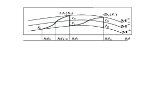
a) b)

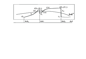
Figure 9: The regular (a) and irregular (b) conservative chain. Dissipative terms for the regular chain give zero balance inside each step. For the irregular chain, dissipative term of part I (the first step) annihilates with dissipative term of part IV (the second step), as well, as annihilate dissipartive terms for parts II and III.

Irregular conservative chain

The regular geometric picture is nice, but for some generalizations we need less rigid structure. Let us combine two operations: the shift in time $\Theta_{\tau}$ and the entropic involution $I_{S}$. Suppose, the motions starts on a point $f_{0}$ on the film of non-equilibrium states, and

$$f_{n+1}=I_{S}(\Theta_{\tau}(f_{n})).$$ (55)

This chain we call an irregular conservative chain, and the chain that moves from ${\bf M^{*}_{-}(s)}$ to ${\bf M^{*}_{+}(s)}$ and back, the regular one. For the regular chain the dissipative term is zero (in the main order in $\tau$) already for one link because this link is symmetric, and the macroscopic entropy ($S(M)$) loose for a motion from ${\bf M^{*}_{-}(s)}$ to ${\bf M^{*}}$ compensate the macroscopic entropy production on a way from ${\bf M^{*}}$ to ${\bf M^{*}_{+}(s)}$. For the irregular chain (55) with given $\tau$ such a compensation occurs in two successive links (Fig. 9b) in main order in $\tau$.

Kinetic modeling for non-zero dissipation. 1. Extension of regular chains

The conservative chain of kinetic curves approximates the quasi-equilibrium dynamics. A typical example of quasi-equilibrium equations (21) is the Euler equation in fluid dynamics. Now, we combine conservative chains construction with the idea of the dissipative Ehrenfests’ chain in order to create a method for kinetic modeling of dissipative hydrodynamics (“macrodynamics”) (39) with arbitrary kinetic coefficient that is decoupled from the chain step $\tau$:

$$\frac{\mathrm{d}M}{\mathrm{d}t}=m(J(f^{*}_{M}))+\kappa(M)m[(D_{f}J(f))_{f=f^{*}_{M}}\Delta_{f^{*}_{M}}].$$ (56)

Here, a kinetic coefficient $\kappa(M)\geq 0$ is a non-negative function of $M$. The entropy production for (10) is:

$$\frac{\mathrm{d}S(M)}{\mathrm{d}t}=\kappa(M)\langle\Delta_{f^{*}_{M}},\Delta_{f^{*}_{M}}\rangle_{f^{*}_{M}}.$$ (57)

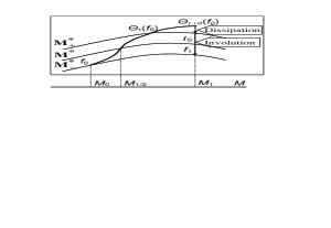
a) b)

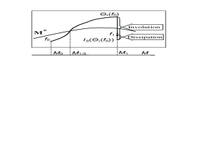
Figure 10: Realization of dissipative chain by the extra time $\vartheta$ on the base of a regular conservative chain (a), and by the incomplete involution on the base of an irregular conservative chain (b).

Let us start from a regular conservative chain and deform it. A chain that approximates solutions of (56) can be constructed as follows (Fig. 10a). The motion starts from $f_{0}\in{\bf M^{*}_{-}(s)}$, goes by a kinetic curve to intersection with ${\bf M^{*}_{+}(s)}$, as for a regular conservative chain, and, after that, follows the same kinetic curve an extra time $\vartheta$. This motion stops at the moment $\tau+\vartheta$ at the point $\Theta_{\tau+\vartheta}(f_{0})$ (Fig. 10a). The second point of the chain, $f_{1}$ is the unique solution of equation

$$m(f_{1})=m(\Theta_{\tau+\vartheta}(f_{0})),\ f_{1}\in{\bf M^{*}_{-}(s)}.$$ (58)

The time step is linked with the kinetic coefficient:

$$\kappa=\frac{\vartheta}{2}+o(\tau+\vartheta).$$ (59)

For entropy production we obtain the analogue of (40)

$$\frac{\mathrm{d}S(M)}{\mathrm{d}t}=\frac{\vartheta}{2}\langle\Delta_{f^{*}_{M}},\Delta_{f^{*}_{M}}\rangle_{f^{*}_{M}}+o(\tau+\vartheta).$$ (60)

All these formulas follow from the first–order picture. In the first order of the time step,

$$q_{M,\tau} = f^{*}_{M}+\tau\Delta_{f^{*}_{M}};$$

$$I_{S}(f^{*}_{M}+\tau\Delta_{f^{*}_{M}}) = f^{*}_{M}-\tau\Delta_{f^{*}_{M}};$$

$$f_{0} = f^{*}_{M_{0}}-\frac{\tau}{2}\Delta_{f^{*}_{M_{0}}};$$

$$\Theta_{t}(f_{0}) = f^{*}_{M(t)}+\left(t-\frac{\tau}{2}\right)\Delta_{f^{*}_{M_{0}}},$$ (61)

and up to the second order of accuracy (that is, again, the first non-trivial term)

$$S(q_{M,\tau})=S(M)+\frac{\tau^{2}}{2}\langle\Delta_{f^{*}_{M}},\Delta_{f^{*}_{M}}\rangle_{f^{*}_{M}}.$$ (62)

For a regular conservative chains, in the first order

$$f_{1}=f^{*}_{M(\tau)}-\frac{\tau}{2}\Delta_{f^{*}_{M_{0}}}.$$ (63)

For chains (58), in the first order

$$f_{1}=f^{*}_{M(\tau+\vartheta)}-\frac{\tau}{2}\Delta_{f^{*}_{M_{0}}}.$$ (64)

Kinetic modeling for non-zero dissipation. 2. Deformed involution in irregular chains

For irregular chains, we introduce dissipation without change of the time step $\tau$. Let us, after entropic involution, shift the point to the quasi-equilibrium state (Fig. 10) with some entropy increase $\sigma(M)$. Because of entropy production formula (57),

$$\sigma(M)=\tau\kappa(M)\langle\Delta_{f^{*}_{M}},\Delta_{f^{*}_{M}}\rangle_{f^{*}_{M}}.$$ (65)

This formula works, if there is sufficient amount of non-equilibrium entropy, the difference $S(M_{n})-S(f_{n})$ should not be too small. In average, for several (two) successive steps it should not be less than $\sigma(M)$. The Ehrenfests’ chain gives a limit for possible value of $\kappa(M)$ that we can realize using irregular chains with overrelaxation:

$$\kappa(M)<\frac{\tau}{2}.$$ (66)

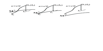
Figure 11: The Ehrenfests’ limit of dissipation: three possible links of a dissipative chain: overrelaxation, $\kappa(M)<\frac{\tau}{2}$ ($\langle\sigma\rangle=s_{\tau}-2\sqrt{s_{\tau}\langle s_{0}\rangle}$), Ehrenfests’ chain, $\kappa(M)=\frac{\tau}{2}$ ($\sigma=s_{\tau}$), and underrelaxation, $\kappa(M)>\frac{\tau}{2}$ ($\langle\sigma\rangle=s_{\tau}+2\sqrt{s_{\tau}\langle s_{0}\rangle}$).

Let us call the value $\kappa(M)=\frac{\tau}{2}$ the Ehrenfests’ limit. Formally, it is possible to realize a chain of kinetic curves with time step $\tau$ for $\kappa(M)>\frac{\tau}{2}$ on the other side of the Ehrenfests’ limit, without overrelaxation (Fig. 11).

Let us choose the following notation for non-equilibrium entropy: $s_{0}=S(M_{0})-S(f_{0})$, $s_{1}=S(M_{1})-S(f_{1})$, $s_{\tau}(M)=\frac{\tau^{2}}{2}{\langle\Delta_{f^{*}_{M}},\Delta_{f^{*}_{M}}\rangle_{f^{*}_{M}}}$. For the three versions of steps (Fig. 11) the entropy gain $\sigma=s(f_{1})-S(I_{S}(\Theta_{\tau}(f_{0})))$ in the main order in $\tau$ is:

• For overrelaxation ($\kappa(M)<\frac{\tau}{2}$) $\sigma=s_{\tau}+s_{0}-s_{1}-2\sqrt{s_{\tau}s_{0}}$;

• For the Ehrenfests’ chain (full relaxation, $\kappa(M)=\frac{\tau}{2}$) $s_{0}=s_{1}=0$ and $\sigma=s_{\tau}$;

• For underrelaxation ($\kappa(M)>\frac{\tau}{2}$) $\sigma=s_{\tau}+s_{0}-s_{1}+2\sqrt{s_{\tau}s_{0}}$.

After averaging in successive steps, the term $s_{0}-s_{1}$ tends to zero, and we can write the estimate of the average entropy gain $\langle\sigma\rangle$: for overrelaxation $\langle\sigma\rangle=s_{\tau}-2\sqrt{s_{\tau}\langle s_{0}\rangle}$ and for underelaxation $\langle\sigma\rangle=s_{\tau}+2\sqrt{s_{\tau}\langle s_{0}\rangle}$.

In the really interesting physical problems the kinetic coefficient $\kappa(M)$ is non-constant in space. Macroscopic variables $M$ are functions of space, $\kappa(M)$ is also a function, and it is natural to take a space-dependent step of macroscopic entropy production $\sigma(M)$. It is possible to organize the involution (incomplete involution) step at different points with different density of entropy production step $\sigma$.

Which entropy rules the kinetic model?

For linear kinetic equations, for example, for the free flight equation (42) there exist many concave Lyapunov functionals (for dissipative systems) or integrals of motion (for conservative systems), see, for example, (4).

There are two reasonable conditions for entropy choice: additivity with respect to joining of independent systems, and trace form (sum or integral of some function $h(f,f^{*})$). These conditions select a one-parametric family ENTR1 ; ENTR3 , a linear combination of the classical Boltzmann–Gibbs–Shannon entropy with $h(f)=-f\ln f$ and the Burg Entropy with $h(f)=\ln f$, both in the Kullback form:

$$S_{\alpha}=-\alpha\int f\ln\frac{f}{f^{*}}\,\mathrm{d}\Gamma(x)+(1-\alpha)\int f^{*}\ln\frac{f}{f^{*}}\,\mathrm{d}\Gamma(x),$$

where $1\geq\alpha\geq 0$, and $f^{*}\mathrm{d}\Gamma$ is invariant measure. Singularity of the Burg term for $f\to 0$ provides the positivity preservation in all entropic involutions.

If we weaken these conditions and require that there exists such a monotonic (nonlinear) transformation of entropy scale that in one scale entropy is additive, and in transformed one it has a trace form, then we get additionally a family of Renyi–Tsallis entropies with $h(f)=\frac{1-f^{q}}{1-q}$ ENTR3 (these entropies and their applications are discussed in details in Abe ).

Both the Renyi–Tsallis entropy and the Burge entropy are in use in the entropic lattice Boltzmann methods from the very beginning ELB1 ; Boghos . The connection of this entropy choice with Galilei invariance is demonstrated in Boghos .

Elementary examples

In the most popular and simple example, the conservative formal kinetic equations (12) is the free flight equation (42). Macroscopic variables $M$ are the hydrodynamic fields: $n(\mbox{\boldmath$x$})=\int f(\mbox{\boldmath$x$},\mbox{\boldmath$v$})\,\mathrm{d}\mbox{\boldmath$v$}$, $n(\mbox{\boldmath$x$})\mbox{\boldmath$u$}(\mbox{\boldmath$x$})=\int\mbox{\boldmath$v$}f(\mbox{\boldmath$x$},\mbox{\boldmath$v$})\,\mathrm{d}\mbox{\boldmath$v$}$, $3n(\mbox{\boldmath$x$})k_{\rm B}T/2m=\frac{1}{2}\int\mbox{\boldmath$v$}^{2}f(\mbox{\boldmath$x$},\mbox{\boldmath$v$})\,\mathrm{d}\mbox{\boldmath$v$}-\frac{1}{2}n(\mbox{\boldmath$x$})\mbox{\boldmath$u$}^{2}(\mbox{\boldmath$x$})$, where $m$ is particle mass. In 3D at any space point we have five independent variables.

For a given value of five macroscopic variables $M=\{n,\mbox{\boldmath$u$},T\}$ (3D), the quasi-equilibrium distribution is the classical local Maxwellian:

$$f^{*}_{M}(\mbox{\boldmath$x$},\mbox{\boldmath$v$})=n\left({2\pi k_{\rm B}T\over m}\right)^{-3/2}\exp\left(-{m(\mbox{\boldmath$v$}-\mbox{\boldmath$u$})^{2}\over 2k_{\rm B}T}\right),$$ (67)

The standard choice of entropy for this example is the classical Boltzmann–Gibbs–Shannon entropy (5) with entropy density $s(\mbox{\boldmath$x$})$. All the involution operations are performed pointwise: at each point $x$ we calculate hydrodynamic moments $M$, the correspondent local Maxwellian (67) $f^{*}_{M}$, and find the entropic inversion at this point with the standard entropy. For dissipative chains, it is useful to take the dissipation (the entropy density gain in one step) proportional to the $S(M)-S(f)$, and not with fixed value.

The special variation of the discussed example is the free flight with finite number of velocities: $f(\mbox{\boldmath$x$},\mbox{\boldmath$v$})=\sum_{i}f_{i}(\mbox{\boldmath$x$})\delta(\mbox{\boldmath$v$}-\mbox{\boldmath$v$}_{i})$. Free flight does not change the set of velocities $\{\mbox{\boldmath$v$}_{1},\ldots\ldots\mbox{\boldmath$v$}_{n}\}$. If we define entropy, then we can define an equilibrium distribution for this set of velocity too. For the entropy definition let us substitute $\delta$-functions in expression for $f(\mbox{\boldmath$x$},\mbox{\boldmath$v$})$ by some “drops” with unite volume, small diameter, and fixed density that may depend on $i$. After that, the classical entropy formula unambiguously leads to expression:

$$s(\mbox{\boldmath$x$})=-\sum_{i}f_{i}(\mbox{\boldmath$x$})\left(\ln\frac{f_{i}(\mbox{\boldmath$x$})}{f^{0}_{i}}-1\right).$$ (68)

This formula is widely known in chemical kinetics (see elsewhere, for example G1 ; Ocherki ; YBGE ). After classical work of Zeldovich Zeld (1938), this function is recognized as a useful instrument for analysis of chemical kinetic equations. Vector of values $f^{0}=f^{0}_{i}$ gives us a “particular equilibrium:” for $M=m(f^{0})$ the conditional equilibrium ($s\to\max$, $M=m(f^{0})$) is $f^{0}$. With entropy (68) we can construct all types of conservative and dissipative chains for discrete set of velocities. If we need to approximate the continuous local equilibria and involutions by our discrete equilibria and involutions, then we should choose a particular equilibrium distribution $\sum_{i}f^{0}_{i}\delta(\mbox{\boldmath$v$}-\mbox{\boldmath$v$}_{i})$ in velocity space as an approximation to the Maxwellian $f^{*0}(\mbox{\boldmath$v$})$ with correspondent value of macroscopic variables $M^{0}$ calculated for the discrete distribution $f^{0}$: $n=\sum_{i}f^{0}_{i}$, … This approximation of distributions should be taken in the weak sense. It means that $\mbox{\boldmath$v$}_{i}$ are nodes, and $f^{0}_{i}$ are weights for a cubature formula in 3D space with weight $f^{*0}(\mbox{\boldmath$v$})$:

$$\int p(\mbox{\boldmath$v$})f^{*0}(\mbox{\boldmath$v$})\,\mathrm{d}\mbox{\boldmath$v$}\approx\sum_{i}p(\mbox{\boldmath$v$}_{i})f^{0}_{i}.$$ (69)

There exist a huge population of cubature formulas in 3D with Gaussian weight that are optimal in various senses cubature . Each of them contains a hint for a choice of nodes $\mbox{\boldmath$v$}_{i}$ and weights $f^{0}_{i}$ for the best discrete approximation of continuous dynamics. Applications of this entropy (68) to the lattice Boltzmann models are developed in LBperfect .

There is one more opportunity to use entropy (68) and related involutions for discrete velocity systems. If for some of components $f_{i}=0$, then we can find the correspondent positive equilibrium, and perform the involution in the whole space. But there is another way: if for some of velocities $f_{i}=0$, then we can reduce the space, and find an equilibrium for non-zero components only, for the shortened list of velocities. These boundary equilibria play important role in the chemical thermodynamic estimations Kagan .

This approach allows us to construct systems with variable in space set of velocities. There could be “soft particles” with given velocities, and the density distribution in these particles changes only when several particles collide. In 3D for the possibility of a non-trivial equilibrium that does not obligatory coincide with the current distribution we need more than 5 different velocity vectors, hence, a non-trivial collision ($\approx$ entropic inversion) is possible only for 6 one-velocity particles. If in a collision participate 5 one-velocity particles or less, then they are just transparent and don’t interact at all. For more moments, if we add some additional fields (stress tensor, for example), the number of velocity vectors that is necessary for non-trivial involution increases.

Lattice Boltzmann models: lattice is not a tool for discretization

In this section, we presented the theoretical backgrounds of kinetic modeling. These problems were discussed previously for development of lattice Boltzmann methods in computational fluid dynamics. The “overrelaxation” appeared in Succi89 . In papers LBGK1 ; LBGK2 the overrelaxation based method for the Navier–Stokes equations was further developed, and the entropic involution was invented in ELB1 . Due to historical reasons, we propose to call it the Karlin–Succi involution. The problem of computational stability of entropic lattice Boltzmann methods was systematically analyzed in LBperfect ; LBentr . $H$-theorem for lattice Boltzmann schemes was presented with details and applications in LB3 . For further discussion and references we address to LB2 .

In order to understand links from the Ehrenfests’ chains to the lattice Boltzmann models, let us take the model with finite number of velocity vectors and entropy (68). Let the velocities from the set $\{\mbox{\boldmath$v$}_{1},\ldots\ldots\mbox{\boldmath$v$}_{n}\}$ be automorphisms of some lattice $\mathbf{L}$: $\mathbf{L}+\mbox{\boldmath$v$}_{i}=\mathbf{L}$. Then the restriction of free flight in time $\tau$ on the functions on the lattice $\tau\mathbf{L}$ is exact. It means that the free flight shift in time $\tau$, $f(x,v)\mapsto f(x-v\tau,v)$ is defined on functions on the lattice, because $\mbox{\boldmath$v$}_{i}\tau$ are automorphisms of $\tau\mathbf{L}$. The entropic involution (complete or incomplete one) acts pointwise, hence, the restriction of the chains on the lattice $\tau\mathbf{L}$ is exact too. In that sense, the role of lattice here is essentially different from the role of grid in numerical methods for PDE. All the discretization contains in the velocity set $\{\mbox{\boldmath$v$}_{1},\ldots\ldots\mbox{\boldmath$v$}_{n}\}$, and the accuracy of discretization is the accuracy of cubature formulas (69).

The lattice $\tau\mathbf{L}$ is a tool for presentation of velocity set as a subset of $\mathbf{L}$ automorphism group. At the same time, it is a perfect screen for presentation of the chain dynamics, because restriction of that dynamics on this lattice is an autonomous dynamic of lattice distribution. (Here we meet a rather rare case of exact model reduction.)

The boundary conditions for the lattice Boltzmann models deserve special attention. There were many trials of non-physical conditions until the proper (and absolutely natural) discretization of well-known classical kinetic boundary conditions (see, for example, Cercignani ) were proposed AK4 . It is necessary and sufficient just to describe scattering of particles on the boundary with maximal possible respect to the basic physics (and given proportion between elastic collisions and thermalization).

3 Coarse-graining by filtering

The most popular area for filtering applications in mathematical physics is the Large Eddy Simulation (LES) in fluid dynamics LES2005 . Perhaps, the first attempt to turbulence modeling was done by Boussinesq in 1887. After that, Taylor (1921, 1935, 1938) and Kolmogorov (1941) have provided the bases of the statistical theory of turbulence. The Kolmogorov theory of turbulence self similarity inspired many attempts of so-called subgrid-scale modeling (SGS model): only the large scale motions of the flow are solved by filtering out the small and universal eddies. For the dynamic subgrid-scale models a filtering step is required to compute the SGS stress tensor. The filtering a hydrodynamic field is defined as convoluting the field functions with a filtering kernel, as it is done in electrical engineering:

$$\overline{\{n,n\mbox{\boldmath$u$},nT\}}(\mbox{\boldmath$x$})=\int G(\mbox{\boldmath$x$}-\mbox{\boldmath$y$}){\{n,n\mbox{\boldmath$u$},nT\}}(\mbox{\boldmath$y$})\,\mathrm{d}\mbox{\boldmath$y$}.$$ (70)

Various filter kernels are in use. Most popular of them are:

1. The box filter $G(x)=H(\Delta/2-|x|)/\Delta$;

2. The Gaussian filter $G(x)=\frac{1}{\Delta}\sqrt{6/\pi}\exp{(-6x^{2}/\Delta^{2})}$,

where $\Delta$ is the filter width (for the Gaussian filter, $\Delta/2=\sqrt{3}\sigma$, this convention corresponds to 91.6% of probability in the interval $[-\Delta/2,+\Delta/2]$ for the Gaussian distribution) , $H$ is the Heaviside function, $G(\mbox{\boldmath$x$})=\prod_{i}G(x_{i})$.

In practical applications, implicit filtering is sometimes done by the grid itself. This filtering by grids should be discussed in context of the Whittaker–Nyquist–Kotelnikov–Shannon sampling theory Higgins1 ; Higgins2 . Bandlimited functions (that is, functions which Fourier transform has compact support) can be exactly reconstructed from their values on a sufficiently fine grid by the Nyquist-Shannon interpolation formula and its multidimensional analogues. If, in 1D, the Fourier spectrum of $f(x)$ belongs to the interval $[-k_{\max},k_{\max}]$, and the grid step $h$ is less than $\pi/k_{\max}$ (it is, twice less than the minimal wave length), then this formula gives the exact representation of $f(x)$ for all points $x$:

$$f(x)=\sum_{n=-\infty}^{+\infty}f(nh){\rm sinc}\left(\pi\left[\frac{x}{h}-n\right]\right),$$ (71)

where ${\rm sinc}(x)=\frac{\sin x}{x}$. That interpolation formula implies an exact differentiation formula in the nodes:

$$\left.\frac{\mathrm{d}f(x)}{\mathrm{d}x}\right|_{x=nh}=2\pi\sum_{k=1}^{\infty}(-1)^{k+1}\frac{f((n+k)h)-f((n-k)h)}{2kh}.$$ (72)

Such “long tail” exact differentiation formulas are useful under assumption about bounded Fourier spectrum.

As a background for SGS modeling, the Boussinesq hypothesis is widely used. This hypothesis is that the turbulent terms can be modeled as directly analogues to the molecular viscosity terms using a “turbulent viscosity.” Strictly speaking, no hypothesis are needed for equation filtering, and below a sketch of exact filtering theory for kinetic equations is presented. The idea of reversible regularization without apriory closure assumptions in fluid dynamics was proposed by Leray Leray . Now it becomes popular again Germano2 ; Holm ; toyLeonard .

3.1 Filtering as auxiliary kinetics

Idea of filtering in kinetics

The variety of possible filters is too large, and we need some fundamental conditions that allow to select physically reasonable approach.

Let us start again from the formal kinetic equation (12) ${\mathrm{d}f}/{\mathrm{d}t}=J(f)$ with concave entropy functional $S(f)$ that does not increase in time and is defined in a convex subset $U$ of a vector space $E$.

The filter transformation $\Phi_{\Delta}:U\to U$, where $\Delta$ is the filter width, should satisfy the following conditions:

1. Preservation of conservation laws: for any basic conservation law of the form $C[f]={\rm const}$ filtering does not change the value $C[f]$: $C[\Phi_{\Delta}(f)]=C[f]$. This condition should be satisfied for the whole probability or for number of particles (in most of classical situations), momentum, energy, and filtering should not change the center of mass, this is not so widely known condition, but physically obvious consequence of Galilei invariance.

2. The Second Law (entropy growth): $S(\Phi_{\Delta}(f))\geq S(f)$.

It is easy to check the conservation laws for convoluting filters (70), and here we find the first benefit from the kinetic equation filtering: for usual kinetic equations and all mentioned conservation laws functionals $C[f]$ are linear, and the conservation preservation conditions are very simple linear restrictions on the kernel $G$ (at least, far from the boundary). For example, for the Boltzmann ideal gas distribution function $f(\mbox{\boldmath$x$},\mbox{\boldmath$v$})$, the number of particles, momentum, and energy conserve in filtering $\overline{f(\mbox{\boldmath$x$},\mbox{\boldmath$v$})}=\int G(\mbox{\boldmath$x$}-\mbox{\boldmath$y$})f(\mbox{\boldmath$y$},\mbox{\boldmath$v$})\,\mathrm{d}\mbox{\boldmath$y$}$, if $\int G(\mbox{\boldmath$x$})\,\mathrm{d}\mbox{\boldmath$x$}=1$; for the center of mass conservation we need also a symmetry condition $\int\mbox{\boldmath$x$}G(\mbox{\boldmath$x$})\,\mathrm{d}\mbox{\boldmath$x$}=0$. It is necessary to mention that usual filters extend the support of distribution, hence, near the boundary the filters should be modified, and boundary can violate the Galilei invariance, as well, as momentum conservation. We return to these problems in this paper later.

For continuum mechanics equations, energy is not a linear functional, and operations with filters require some accuracy and additional efforts, for example, introduction of spatially variable filters Vreman . Perhaps, the best way is to lift the continuum mechanics to kinetics, to filter the kinetic equation, and then to return back to filtered continuum mechanics. On kinetic level, it becomes obvious how filtering causes the redistribution of energy between internal energy and mechanical energy: energy of small eddies and of other small-scale inhomogeneities partially migrates into internal energy.

Filtering semigroup

If we apply the filtering twice, it should lead just just to increase of the filter width. This natural semigroup condition reduces the set of allowed filters significantly. The approach based on filters superposition was analyzed by Germano Germano and developed by many successors. Let us formalize it in a form

$$\Phi_{\Delta^{\prime}}(\Phi_{\Delta}(f))=\Phi_{\Delta^{\prime\prime}}(f),$$ (73)

where $\Delta^{\prime\prime}(\Delta^{\prime},\Delta)$ is a monotonic function, $\Delta^{\prime\prime}\geq\Delta^{\prime}$ and $\Delta^{\prime\prime}\geq\Delta$.

The semigroup condition (73) holds for the Gaussian filter with $\Delta^{\prime\prime 2}=\Delta^{\prime 2}+\Delta^{2}$, and does not hold for the box filter. It is convenient to parameterize the semigroup $\{\Phi_{\Delta}|\Delta\geq 0\}$ by an additive parameter $\eta\geq 0$ (“auxiliary time”): $\Delta=\Delta(\eta)$, $\Phi_{\eta}\circ\Phi_{\eta^{\prime}}=\Phi_{\eta+\eta^{\prime}}$, $\Phi_{0}={\rm id}$. Further we use this parameterization.

Auxiliary kinetic equation

The filtered distribution $f(\eta)=\Phi_{\eta}(f_{0})$ satisfies differential equation

$$\frac{\mathrm{d}f(\eta)}{\mathrm{d}\eta}=\phi(f(\eta)),\;\mbox{where}\;\phi(f)=\lim_{\eta\to 0}\frac{\Phi_{\eta}(f)-f}{\eta}.$$ (74)

For Gaussian filters this equation is the simplest diffusion equation ${\mathrm{d}f(\eta)}/{\mathrm{d}\eta}={\rm\Delta}f$ (here ${\rm\Delta}$ is the Laplace operator).

Due to physical restrictions on possible filters, auxiliary equation (74) has main properties of kinetic equations: it respects conservation laws and the Second Law. It is also easy to check that in the whole space (without boundary effects) diffusion, for example, does not change the center of mass.

So, when we discuss filtering of kinetics, we deal with two kinetic equations in the same space, but in two times $t$ and $\eta$: initial kinetics (12) and filtering equation (74). Both have the same conservation laws and the same entropy.

3.2 Filtered kinetics

Filtered kinetic semigroup

Let $\Theta_{t}$ be the semigroup of the initial kinetic phase flow. We are looking for kinetic equation that describes dynamic of filtered distribution $\Phi_{\eta}f$ for given $\eta$. Let us call this equation with correspondent dynamics the filtered kinetics. It is the third kinetic equation in our consideration, in addition to the initial kinetics (12) and the auxiliary filtering kinetics (74). The natural phase space for this filtered kinetics is the set of filtered distributions $\Phi_{\eta}(U)$. For the phase flow of the filtered kinetics we use notation $\Psi_{(\eta)\,t}$ This filtered kinetics should be the exact shadow of the true kinetics. It means that the motion $\Psi_{(\eta)\,t}(\Phi_{\eta}f_{0})$ is the result of filtering of the true motion $\Theta_{t}(f_{0})$: for any $f_{0}\in U$ and $t>0$

$$\Psi_{(\eta)\,t}(\Phi_{\eta}f_{0})=\Phi_{\eta}(\Theta_{t}(f_{0})).$$ (75)

This equality means that

$$\Psi_{(\eta)\,t}=\Phi_{\eta}\circ\Theta_{t}\circ\Phi_{-\eta}$$ (76)

The transformation $\Phi_{-\eta}$ is defined on the set of filtered distributions $\Phi_{\eta}(U)$, as well as $\Psi_{(\eta)\,t}$ is. Now it is necessary to find the vector field

$$\psi_{(\eta)}(f)=\left.\frac{\mathrm{d}\Psi_{(\eta)\,t}(f)}{\mathrm{d}t}\right|_{t=0}$$

on the base of conditions (75), (76). This vector field is the right-hand side of the filtered kinetic equations

$$\frac{\mathrm{d}f}{\mathrm{d}t}=\psi_{(\eta)}(f).$$ (77)

From (76) immediately follows:

$$\frac{\mathrm{d}\psi_{(\eta)}(f)}{\mathrm{d}\eta}=(D_{f}\phi(f))\psi_{(\eta)}(f)-(D_{f}\psi_{(\eta)}(f))\phi(f)=[\psi_{(\eta)},\phi](f),$$ (78)

where $[\psi,\phi]$ is the Lie bracket of vector fields.

In the first approximation in $\eta$

$$\psi_{(\eta)}(f)=J(f)+\eta((D_{f}\phi(f))J(f)-(D_{f}J(f))\phi(f))=J(f)+\eta[J,\phi](f),$$ (79)

the Taylor series expansion for $\psi_{(\eta)}(f)$ is

$$\psi_{(\eta)}(f)=J(f)+\eta[J,\phi](f)+\frac{\eta^{2}}{2}[[J,\phi],\phi](f)+\ldots+\frac{\eta^{n}}{n!}[\ldots[J,\underbrace{\phi],...\phi]}_{n}(f)+\ldots$$ (80)

We should stress again that filtered equations (77) with vector field $\psi_{(\eta)}(f)$ that satisfies (78) is exact and presents just a shadow of the original kinetics. Some problems may appear (or not) after truncating the Taylor series (80), or after any other approximation.

So, we have two times: physical time $t$ and auxiliary filtering time $\eta$, and four different equations of motion in these times:

• initial equation (12) (motion in time $t$),

• filtering equation (74) (motion in time $\eta$),

• filtered equation (77) (motion in time $t$),

• and equation for the right hand side of filtered equation (78) (motion in time $\eta$).

Toy example: advection + diffusion

Let us consider kinetics of system that is presented by one scalar density in space (concentration), with only one linear conservation law, the total number of particles.

In the following example the filtering equation (74) is

$$\frac{\partial f(\mbox{\boldmath$x$},\eta)}{\partial\eta}={\rm\Delta}f(\mbox{\boldmath$x$},\eta)\>(=\phi(f)).$$ (81)

The differential of $\phi(f)$ is simply the Laplace operator ${\rm\Delta}$. The correspondent 3D heat kernel (the fundamental solution of (81)) is

$$K(\eta,\mbox{\boldmath$x$}-\mbox{\boldmath$\xi$})=\frac{1}{(4\pi\eta)^{3/2}}\exp\left(-\frac{(\mbox{\boldmath$x$}-\mbox{\boldmath$\xi$})^{2}}{4\eta}\right).$$ (82)

After comparing this kernel with the Gaussian filter we find the filter width $\Delta=\sqrt{24\eta}$.

Here we consider the diffusion equation (81) in the whole space with zero conditions at infinity. For other domains and boundary conditions the filtering kernel is the correspondent fundamental solution.

The equation for the right hand side of filtered equation (78) is

$$\frac{\mathrm{d}\psi_{(\eta)}(f)}{\mathrm{d}\eta}={\rm\Delta}(\psi_{(\eta)}(f))-(D_{f}\psi_{(\eta)}(f))({\rm\Delta}f)\>(=[\psi,\phi](f)).$$ (83)

For the toy example we select the advection + diffusion equation

$$\frac{\partial f(\mbox{\boldmath$x$},t)}{\partial t}=\kappa{\rm\Delta}f(\mbox{\boldmath$x$},t)-{\rm div}(\mbox{\boldmath$v$}(\mbox{\boldmath$x$})f(\mbox{\boldmath$x$},t))\>(=J(f)).$$ (84)

where $\kappa>0$ is a given diffusion coefficient, $\mbox{\boldmath$v$}(\mbox{\boldmath$x$})$ is a given velocity field. The differential $D_{f}J(f)$ is simply the differential operator from the right hand side of (84), because this vector field is linear. After simple straightforward calculation we obtain the first approximation (79) to the filtered equation:

$$[J,\phi](f) = {\rm\Delta}(J(f))-(D_{f}J(f))({\rm\Delta}f)=-{\rm\Delta}[{\rm div}(\mbox{\boldmath$v$}f)]+{\rm div}(\mbox{\boldmath$v$}{\rm\Delta}f)$$

$$= {\rm div}[\mbox{\boldmath$v$}{\rm\Delta}f-{\rm\Delta}(\mbox{\boldmath$v$}f)]=-{\rm div}\left[f{\rm\Delta}\mbox{\boldmath$v$}+2\sum_{r}\frac{\partial\mbox{\boldmath$v$}}{\partial x_{r}}\frac{\partial f}{\partial x_{r}}\right]$$

$$= -{\rm div}(f{\rm\Delta}\mbox{\boldmath$v$})-\sum_{i}\frac{\partial}{\partial x_{i}}\left[\sum_{r}\left(\frac{\partial v_{i}}{\partial x_{r}}+\frac{\partial v_{r}}{\partial x_{i}}\right)\frac{\partial f}{\partial x_{r}}\right.$$

$$\left.-\sum_{r}\frac{\partial f}{\partial x_{r}}\left(\frac{\partial v_{i}}{\partial x_{r}}-\frac{\partial v_{r}}{\partial x_{i}}\right)\right]$$

$$= -\sum_{i}\frac{\partial}{\partial x_{i}}\left[\sum_{r}\left(\frac{\partial v_{i}}{\partial x_{r}}+\frac{\partial v_{r}}{\partial x_{i}}\right)\frac{\partial f}{\partial x_{r}}\right]-\sum_{r}\frac{\partial}{\partial x_{r}}\left(f\frac{\partial{\rm div}\mbox{\boldmath$v$}}{\partial x_{r}}\right).$$

The resulting equations in divergence form are

$$\frac{\partial f(\mbox{\boldmath$x$},t)}{\partial t} = J(f)+\eta[J,\phi](f)$$

$$= -{\rm div}\left(-\kappa\nabla f+(\mbox{\boldmath$v$}+\eta{\rm\Delta}\mbox{\boldmath$v$})f+2\eta\sum_{r}\frac{\partial\mbox{\boldmath$v$}}{\partial x_{r}}\frac{\partial f}{\partial x_{r}}\right)$$

$$= {\rm div}((\kappa-2\eta\mbox{\boldmath$S$}(\mbox{\boldmath$x$}))\nabla f(\mbox{\boldmath$x$},t))-{\rm div}((\mbox{\boldmath$v$}(\mbox{\boldmath$x$})+\eta\nabla{\rm div}\mbox{\boldmath$v$}(\mbox{\boldmath$x$}))f(\mbox{\boldmath$x$},t)),$$

where $\mbox{\boldmath$S$}(\mbox{\boldmath$x$})=(S_{ij})=\frac{1}{2}\left(\frac{\partial v_{i}}{\partial x_{j}}+\frac{\partial v_{j}}{\partial x_{i}}\right)$ is the strain tensor. In filtered equations (3.2) the additional diffusivity tensor $-2\eta\mbox{\boldmath$S$}(\mbox{\boldmath$x$})$ and the additional velocity $\eta\nabla{\rm div}\mbox{\boldmath$v$}(\mbox{\boldmath$x$})$ are present. The additional diffusivity tensor $-2\eta\mbox{\boldmath$S$}(\mbox{\boldmath$x$})$ may be not positive definite. The positive definiteness of the diffusivity tensor $\kappa-2\eta\mbox{\boldmath$S$}(\mbox{\boldmath$x$})$ may be also violated. For arbitrary initial condition $f_{0}(\mbox{\boldmath$x$})$ it may cause some instability problems, but we should take into account that the filtered equations (3.2) are defined on the space of filtered functions for given filtering time $\eta$. On this space the negative diffusion ($\partial_{t}f=-{\rm\Delta}f$) is possible during time $\eta$. Nevertheless, the approximation of exponent (80) by the linear term (79) can violate the balance between smoothed initial conditions and possible negative diffusion and can cause some instabilities.

Some numerical experiments with this model (3.2) for incompressible flows (${\rm div}\mbox{\boldmath$v$}=0$) are presented in toyLeonard .

Let us discuss equation (83) in more details. We shall represent it as the dynamics of the filtered advection flux vector $\Pi$. The filtered equation for any $\eta$ should have the form: ${\partial f}/{\partial t}=-{\rm div}(-\kappa\nabla f+\mbox{\boldmath$\Pi$}(f))$, where

$$\mbox{\boldmath$\Pi$}(f)=\left(\sum_{j_{1},j_{2},j_{3}\geq 0}\mbox{\boldmath$a$}_{j_{1}j_{2}j_{3}}(\mbox{\boldmath$x$},\eta)\partial^{j_{1}j_{2}j_{3}}_{x}\right)f(\mbox{\boldmath$x$}),$$ (87)

where

$$\partial^{j_{1}j_{2}j_{3}}_{x}=\left(\frac{\partial}{\partial x_{1}}\right)^{j_{1}}\left(\frac{\partial}{\partial x_{2}}\right)^{j_{2}}\left(\frac{\partial}{\partial x_{3}}\right)^{j_{3}}$$ (88)

For coefficients $\mbox{\boldmath$a$}_{j_{1}j_{2}j_{3}}(\mbox{\boldmath$x$},\eta)$ equation (83) is

$$\frac{\partial\mbox{\boldmath$a$}_{j_{1}j_{2}j_{3}}(\mbox{\boldmath$x$},\eta)}{\partial\eta} = {\rm\Delta}\mbox{\boldmath$a$}_{j_{1}j_{2}j_{3}}(\mbox{\boldmath$x$},\eta)$$

$$+ 2\frac{\partial\mbox{\boldmath$a$}_{j_{1}-1\,j_{2}j_{3}}(\mbox{\boldmath$x$},\eta)}{\partial x_{1}}+2\frac{\partial\mbox{\boldmath$a$}_{j_{1}j_{2}-1\,j_{3}}(\mbox{\boldmath$x$},\eta)}{\partial x_{2}}+2\frac{\partial\mbox{\boldmath$a$}_{j_{1}j_{2}j_{3}-1}(\mbox{\boldmath$x$},\eta)}{\partial x_{3}}.$$

The initial conditions are: $\mbox{\boldmath$a$}_{000}(\mbox{\boldmath$x$},0)=\mbox{\boldmath$v$}(\mbox{\boldmath$x$})$, $\mbox{\boldmath$a$}_{j_{1}j_{2}j_{3}}(\mbox{\boldmath$x$},0)=0$ if at least one of $j_{k}>0$. Let us define formally $\mbox{\boldmath$a$}_{j_{1}j_{2}j_{3}}(\mbox{\boldmath$x$},\eta)\equiv 0$ if at least one of $j_{k}$ is negative.

We shall consider (3.2) in the whole space with appropriate conditions at infinity. There are many representation of solution to this system. Let us use the Fourier transformation:

$$\frac{\partial\hat{\mbox{\boldmath$a$}}_{j_{1}j_{2}j_{3}}(\mbox{\boldmath$k$},\eta)}{\partial\eta}=-k^{2}\hat{\mbox{\boldmath$a$}}_{j_{1}j_{2}j_{3}}(\mbox{\boldmath$k$},\eta)$$ (90)

$$+2i(k_{1}\hat{\mbox{\boldmath$a$}}_{j_{1}-1\,j_{2}j_{3}}(\mbox{\boldmath$k$},\eta)+k_{2}\hat{\mbox{\boldmath$a$}}_{j_{1}j_{2}-1\,j_{3}}(\mbox{\boldmath$k$},\eta)+k_{3}\hat{\mbox{\boldmath$a$}}_{j_{1}j_{2}j_{3}-1}(\mbox{\boldmath$k$},\eta)).$$

Elementary straightforward calculations give us:

$$\hat{\mbox{\boldmath$a$}}_{j_{1}j_{2}j_{3}}(\mbox{\boldmath$k$},\eta)=(2i\eta)^{|j|}{\rm e}^{-k^{2}\eta}\frac{k_{1}^{j_{1}}k_{2}^{j_{2}}k_{3}^{j_{3}}}{j_{1}!j_{2}!j_{3}!}\hat{\mbox{\boldmath$v$}}(\mbox{\boldmath$k$}),$$ (91)

where $|j|=j_{1}+j_{2}+j_{3}$. To find this answer, we consider all monotonic paths on the integer lattice from the point $(0,0,0)$ to the point $(j_{1},j_{2},j_{3})$. In concordance with (90), every such a path adds a term

$$\frac{(2i\eta)^{|j|}}{|j|!}{\rm e}^{-k^{2}\eta}k_{1}^{j_{1}}k_{2}^{j_{2}}k_{3}^{j_{3}}\hat{\mbox{\boldmath$v$}}(\mbox{\boldmath$k$})$$

to $\hat{\mbox{\boldmath$a$}}_{j_{1}j_{2}j_{3}}(\mbox{\boldmath$k$},\eta)$. The number of these paths is $|j|!/(j_{1}!j_{2}!j_{3}!)$.

The inverse Fourier transform gives

$$\mbox{\boldmath$a$}_{j_{1}j_{2}j_{3}}(\mbox{\boldmath$x$},\eta)=(2\eta)^{|j|-3/2}\frac{\partial^{j_{1}j_{2}j_{3}}_{x}}{{j_{1}!j_{2}!j_{3}!}}\int\exp-\frac{(\mbox{\boldmath$x$}-\mbox{\boldmath$y$})^{2}}{4\eta}\mbox{\boldmath$v$}(\mbox{\boldmath$y$})\,\mathrm{d}\mbox{\boldmath$y$}.$$ (92)

Finally, for $\Pi$ we obtain

$$\mbox{\boldmath$\Pi$}(f)$$ (93)

$$=\sum_{j_{1},j_{2},j_{3}\geq 0}\frac{(2\eta)^{|j|-3/2}}{j_{1}!j_{2}!j_{3}!}\left(\partial^{j_{1}j_{2}j_{3}}_{x}\int\exp-\frac{(\mbox{\boldmath$x$}-\mbox{\boldmath$y$})^{2}}{4\eta}\mbox{\boldmath$v$}(\mbox{\boldmath$y$})\,\mathrm{d}\mbox{\boldmath$y$}\,\right)\partial^{j_{1}j_{2}j_{3}}_{x}f(\mbox{\boldmath$x$}).$$

By the way, together with (93) we received the following formula for the Gaussian filtering of products toyLeonard . If the semigroup $\Phi_{\eta}$ is generated by the diffusion equation (81), then for two functions $f(\mbox{\boldmath$x$}),g(\mbox{\boldmath$x$})$ in $R^{n}$ (if all parts of the formula exist):

$$\Phi_{\eta}(fg)=\sum_{j_{1},j_{2},\ldots j_{n}\geq 0}\frac{(2\eta)^{|j|-n/2}}{j_{1}!j_{2}!\ldots j_{n}!}(\partial^{j_{1}j_{2}\ldots j_{n}}_{x}\Phi_{\eta}(f))(\partial^{j_{1}j_{2}\ldots j_{n}}_{x}\Phi_{\eta}(g)).$$ (94)

Generalization of this formula for a broader class of filtering kernels for convolution filters is described in Carati . This is simply the Taylor expansion of the Fourier transformation of the convolution equality $\Psi_{t}=\Phi\circ\Theta_{t}\circ\Phi^{-1}$, where $\Phi$ is the filtering transformation (see (76)).

For filtering semigroups all such formulas are particular cases of the commutator expansion (80), and calculation of all orders requires differentiation only. This case includes non-convolution filtering semigroups also (for example, solutions of the heat equations in a domain with given boundary conditions, it is important for filtering of systems with boundary conditions), as well as semigroups of non-linear kinetic equation.

Nonlinear filtering toy example

Let us continue with filtering of advection + diffusion equation (84) and accept the standard assumption about incompressibility of advection flow $v$: ${\rm div}\mbox{\boldmath$v$}=0$. The value of density $f$ does not change in motion with the advection flow, and for diffusion the maximum principle exists, hence, it makes sense to study bounded solutions of (84) with appropriate boundary conditions, or in the whole space. Let us take $\max f<A$. This time we use the filtering semigroup

$$\frac{\partial f(\mbox{\boldmath$x$},\eta)}{\partial\eta}=-{\rm div}(-(A-f)\nabla f)=(A-f){\rm\Delta}f(\mbox{\boldmath$x$},\eta)-(\nabla f)^{2}\>(=\phi(f)).$$ (95)

This semigroup has slightly better properties of reverse filtering (at least, no infinity in values of $f$). The first-order filtered equation (79) for this filter is (compare to (3.2):

$$\frac{\partial f(\mbox{\boldmath$x$},t)}{\partial t} = J(f)+\eta[J,\phi](f)$$

$$= -{\rm div}[-\kappa\nabla(f+\eta(\nabla f)^{2})+2\eta(A-f)\mbox{\boldmath$S$}\nabla f+\mbox{\boldmath$v$}f].$$

Here, $S$ is the strain tensor, the term $-2\eta(A-f)\mbox{\boldmath$S$}$ is the additional (nonlinear) tensor diffusivity, and the term $\eta\kappa\nabla(\nabla f)^{2}$ describes the flux from areas with high $f$ gradient. Because this flux vanishes near critical points of $f$, it contributes to creation of a patch structure.

In the same order in $\eta$, it is convenient to write:

$$\frac{\partial f(\mbox{\boldmath$x$},t)}{\partial t}=-{\rm div}[-(\kappa-2\eta(A-f)\mbox{\boldmath$S$})\nabla(f+\eta(\nabla f)^{2})+\mbox{\boldmath$v$}f].$$

The nonlinear filter changes not only the diffusion coefficient, but the correspondent thermodynamic force also: instead of $-\nabla f$ we obtain $-\nabla(f+\eta(\nabla f)^{2})$. This thermodynamic force depends on $f$ gradient and can participate in the pattern formation.

LES + POD filters

In the title, LES stands for Large Eddy Simulation, as it is before, and POD stands for Proper Orthogonal Decomposition. POD POD is an application of principal component analysis princ for extraction of main components from the flow dynamics. The basic procedure is quite simple. The input for POD is a finite set of flow images (a sample) $\{f_{1},\ldots,f_{n}\}$. These images are functions in space, usually we have the values of these function on a grid. In the space of functions an inner product is given. The first choice gives the $L_{2}$ inner product $\int fg\,\mathrm{d}x$, or energetic one, or one of the Sobolev’s space inner products. The mean point $\psi_{0}=\sum_{i}f_{i}/n$ minimizes the sum of distance squares $\sum_{i}(f_{i}-\psi_{0})^{2}$. The first principal component $\psi_{1}$ minimizes the sum of distance squares from points $f_{i}$ to a straight line $\{\psi_{0}+\alpha\psi_{1}\ |\ \alpha\in R\}$, the second principal component, $\psi_{2}$, is orthogonal to $\psi_{1}$ and minimizes the sum of distance squares from points $f_{i}$ to a plain $\{\psi_{0}+\alpha_{1}\psi_{1}+\alpha_{2}\psi_{2}\ |\ \alpha_{1,2}\in R\}$, and so on. Vectors of principal components $\psi_{i}$ are the eigenvectors of the sample covariance matrix $\Sigma$, sorted by decreasing eigenvalue $\lambda_{i}$, where

$$\Sigma=\frac{1}{n}\sum_{i}(f_{i}-\psi_{0})\otimes(f_{i}-\psi_{0})^{T}=\frac{1}{n}\sum_{i}|f_{i}-\psi_{0}\rangle\langle f_{i}-\psi_{0}|.$$ (97)

The projection of a field $f$ on the plane of the $k$ first principal components is $\psi_{0}+P_{k}(f)$, where $P_{k}$ is the orthogonal projector on the space spanned by the first $k$ components:

$$P_{k}(\phi)=\sum_{1\leq j\leq k}\psi_{j}(\psi_{j},\phi).$$ (98)

The average square distance from the sample points $f_{i}$ to the plane of the $k$ first principal components is

$$\sigma_{j}^{2}=\sum_{j>k}\lambda_{j}={\rm tr}\Sigma-\sum_{1\leq j\leq k}\lambda_{j}\;\;\left({\rm tr}\Sigma=\frac{1}{n}\sum_{i}(f_{i}-\psi_{0})^{2}\right).$$ (99)

This number, $\sigma_{j}$, measures the accuracy of substitution of the typical (in this sample) field $f$ by its projection on the plane of the $k$ first principal components.

Among many applications of POD in fluid dynamics at least two have direct relations to the coarse-graining:

• Postprocessing, that is, analysis of an experimentally observed or numerically computed flow regime in projection on the finite-dimensional space of the first principal components;

• Creation of “optimal” Galerkin approximations (Galerkin POD, PODGal ). In this approach, after finding principal components from sampled images of flow, we project the equations on the first principal components, and receive a reduced model.

In addition to radical and irreversible step from initial equations to Galerkin POD, we can use POD filtering semigroup. It suppresses the component of field orthogonal to selected $k$ first principal components, but makes this reversibly. The filtering semigroup is generated by auxiliary equation

$$\frac{\mathrm{d}f(\eta)}{\mathrm{d}\eta}=\phi(f(\eta))=-(1-P_{k})(f-\psi_{0}).$$ (100)

The filter transformation in explicit form is

$$U_{\eta}(f)=\psi_{0}+(P_{k}+{\rm e}^{-\eta}(1-P_{k}))(f-\psi_{0}).$$ (101)

with explicit reverse transformation $U_{-\eta}$.

For equations of the form (12) $\dot{f}=J(f)$, the POD filtered equations are

$$\frac{\mathrm{d}f}{\mathrm{d}t}=(D_{f}U_{\eta}(f))_{U_{-\eta}(f)}(J(U_{-\eta}(f)))=(P_{k}+{\rm e}^{-\eta}(1-P_{k}))(J(U_{-\eta}f)).$$ (102)

These equations have nonconstant in space coefficients, because $P_{k}$ is combined from functions $\psi_{i}$. They are also non-local, because $P_{k}$ includes integration, but this non-locality appears in the form of several inner products (moments) only. Of course, this approach can be combined with usual filtering, nonlinear Galerkin approximations GalTem , and non-linear principal manifold approaches GZComp2005 .

Main example: the BGK model kinetic equation

The famous BGK model equation substitutes the Boltzmann equation in all cases when we don’t care about exact collision integral (and it is rather often, because usually it is difficult to distinguish our knowledge about exact collision kernel from the full ignorance).

For the one-particle distribution function $f(\mbox{\boldmath$x$},\mbox{\boldmath$v$},t)$ the BGK equation reads:

$$\frac{\partial f(\mbox{\boldmath$x$},\mbox{\boldmath$v$},t)}{\partial t}+\sum_{i}v_{i}\frac{\partial f(\mbox{\boldmath$x$},\mbox{\boldmath$v$},t)}{\partial x_{i}}=\frac{1}{\tau_{\rm col}}(f^{*}_{m(f)}(\mbox{\boldmath$x$},\mbox{\boldmath$v$})-f(\mbox{\boldmath$x$},\mbox{\boldmath$v$},t)),$$ (103)

where $m(f)=M(t)$ is the cortege of the hydrodynamic fields that corresponds to $f(\mbox{\boldmath$x$},\mbox{\boldmath$v$},t)$, and $f^{*}_{m(f)}$ is the correspondent local Maxwellian. Let us rescale variables $x,v,t$: we shall measure $x$ in some characteristic macroscopic units $L$, $v$ in units of thermal velocity $v_{T}$ for a characteristic temperature, $t$ in units $L/v_{T}$. Of course, there is no exact definition of the “characteristic time” or length, but usually it works if not take it too serious. After rescaling, the BGK equation remains the same, only the parameter becomes dimensionless:

$$\frac{\partial f(\mbox{\boldmath$x$},\mbox{\boldmath$v$},t)}{\partial t}+\sum_{i}v_{i}\frac{\partial f(\mbox{\boldmath$x$},\mbox{\boldmath$v$},t)}{\partial x_{i}}=\frac{1}{K\!n}(f^{*}_{m(f)}(\mbox{\boldmath$x$},\mbox{\boldmath$v$})-f(\mbox{\boldmath$x$},\mbox{\boldmath$v$},t)),$$ (104)

where $K\!n=l/L$ is the dimensionless Knudsen number (and $l$ is the mean–free–path). It is the small parameter in the kinetics – fluid dynamics transition. If the $K\!n\gtrsim 1$ then the continuum assumption of fluid mechanics is no longer a good approximation and kinetic equations must be used.

It is worth to mention that the BGK equation is non-linear. The term $f^{*}_{m(f)}$ depends non-linearly on moments $m(f)$, and, hence, on the distribution density $f$ too. And $f^{*}_{m(f)}$ is the only term in (103) that don’t commute with the Laplace operator from the filtering equation (81). All other terms do not change after filtering.

According to (79), in the first order in $\eta$ the filtered BGK equation is

$$\frac{\partial f}{\partial t}+\sum_{i}v_{i}\frac{\partial f}{\partial x_{i}}$$ (105)

$$=\frac{1}{K\!n}(f^{*}_{m(f)}-f)+\frac{\eta}{K\!n}(D^{2}_{M}f^{*}_{M})_{M=m(f)}(\nabla M,\nabla M)_{M=m(f)}.$$

The last notation may require some explanations: $(D^{2}_{M}f^{*}_{M})$ is the second differential of $f^{*}_{M}$, for the BGK model equation it is a quadratic form in $R^{5}$ that parametrically depends on moment value $M=\{M_{0},M_{1},M_{2},M_{3},M_{4}\}$. In the matrix form, the last expression is

$$(D^{2}_{M}f^{*}_{M})_{M=m(f)}(\nabla M,\nabla M)_{M=m(f)}$$ (106)

$$\qquad\qquad\qquad\qquad\qquad=\sum_{r=1}^{3}\sum_{i,j=0}^{4}\left(\frac{\partial^{2}f^{*}_{M}}{\partial M_{i}M_{j}}\right)_{M=m(f)}\frac{\partial M_{i}}{\partial x_{r}}\frac{\partial M_{j}}{\partial x_{r}}.$$

This expression depends on the macroscopic fields $M$ only. From identity (20) it follows that the filtering term gives no inputs in the quasi-equilibrium approximation, because $m(D^{2}_{M}f^{*}_{M})=0$.

This fact is a particular case of the general commutation relations for general quasi-equilibrium distributions. Let a linear operator $\mathbf{B}$ acts in the space of distributions $f$, and there exists such a linear operator $\mathbf{b}$ which acts in the space of macroscopic states $M$ that $m\mathbf{B}=\mathbf{b}m$. Then

$$m(\mathbf{B}f^{*}_{m(f)}-(D_{f}f^{*}_{m(f)})(\mathbf{B}f))=0.$$ (107)

This means that the macroscopic projection of the Lie bracket for the vector fields of equations $\partial_{\eta}f=\mathbf{B}f$ (a field $\phi$) and $\partial_{t}f=f^{*}_{m(f)}-f$ (a field $\theta$) is zero: $m([\theta,\phi])=0$. These commutation relations follow immediately from the self-consistency identities (18), (19), if we use relations $m\mathbf{B}=\mathbf{b}m$ to carry $m$ through $\mathbf{B}$. In the case of BGK equation, relations (107) hold for any linear differential or pseudodifferential operator $\mathbf{B}=Q(\mbox{\boldmath$x$},\partial/\partial\mbox{\boldmath$x$})$ that acts on functions of $x$. In this case, $\mathbf{b}=\mathbf{B}$, if we use the same notation for differentiation of functions and of vector-functions.

Relations (107) imply a result that deserves special efforts for physical understanding: the filtered kinetic equations in zero order in the Knudsen number produce the classical Euler equations for filtered hydrodynamic fields without any trace of the filter terms. At the same time, direct filtering of the Euler equation adds new terms.

To obtain the next approximation we need the Chapman–Enskog method for equation (105). We developed a general method for all equations of this type (29), and now apply this method to the filtered BGK equation. Let us take in (26) $\epsilon={K\!n}$, $F(f)=F_{0}(f)+F_{\rm filt}(f)$, where $F_{0}=-\mbox{\boldmath$v$}\partial/\partial\mbox{\boldmath$x$}$ is the free flight operator and

$$F_{\rm filt}(f)=\frac{\eta}{K\!n}(D^{2}_{M}f^{*}_{M})_{M=m(f)}(\nabla M,\nabla M)_{M=m(f)}.$$ (108)

In these notations, for the zero term in the Chapman–Enskog expansion we have $f^{(0)}_{M}=f^{*}_{M}$, and for the first term

$$f^{(1)}_{M}=f^{\rm NS}_{M}+f^{\rm filt}_{M}=\Delta^{\rm NS}_{f^{*}_{M}}+\Delta^{\rm filt}_{f^{*}_{M}},$$ (109)

$$f^{\rm NS}_{M}=\Delta^{\rm NS}_{f^{*}_{M}}=F_{0}(f^{*}_{M})-(D_{M}f^{*}_{M})(m(F_{0}(f^{*}_{M})))$$

$$f^{\rm filt}_{M}=\Delta^{\rm filt}_{f^{*}_{M}}=F_{\rm filt}(f)\;\;({\rm because}\;m(F_{\rm filt}(f))=0),$$

where NS stands for Navier–Stokes. The correspondent continuum equations (30) are

$$\frac{\mathrm{d}M}{\mathrm{d}t}=m(F_{0}(f^{*}_{M}))+{K\!n}\,m(F_{0}(\Delta^{\rm NS}_{f^{*}_{M}}+\Delta^{\rm filt}_{f^{*}_{M}})).$$ (110)

Here, the first term includes non-dissipative terms (the Euler ones) of the Navier–Stokes equations, and the second term includes both the dissipative terms of the Navier–Stokes equations and the filtering terms. Let us collect all the classical hydrodynamic terms together:

$$\frac{\partial M(\mbox{\boldmath$x$},t)}{\partial t} = \underbrace{\ldots\ldots\ldots\ldots}_{\rm NS\,terms}+{K\!n}\,m\!\left(\mbox{\boldmath$v$}\frac{\partial}{\partial\mbox{\boldmath$x$}}F_{\rm filt}(f)\right)$$

$$= \underbrace{\ldots\ldots\ldots\ldots}_{\rm NS\,terms}+\eta m\!\left(\mbox{\boldmath$v$}\frac{\partial}{\partial\mbox{\boldmath$x$}}\sum_{r=1}^{3}\sum_{i,j=0}^{4}\frac{\partial^{2}f^{*}_{M}}{\partial M_{i}M_{j}}\frac{\partial M_{i}}{\partial x_{r}}\frac{\partial M_{j}}{\partial x_{r}}\right),$$

The NS terms here are the right hand sides of the Navier–Stokes equations for the BGK kinetics (2.3) (with $\tau=2\tau_{\rm col}=2{K\!n}$). Of course, (3.2) is one of the tensor viscosity – tensor diffusivity models. Its explicit form for the BGK equation and various similar model equations requires several quadratures:

$$C_{ij}=m\!\left(\mbox{\boldmath$v$}\frac{\partial}{\partial\mbox{\boldmath$x$}}\sum_{r=1}^{3}\sum_{i,j=0}^{4}\frac{\partial^{2}f^{*}_{M}}{\partial M_{i}M_{j}}\right)$$ (112)

(for the Maxwell distributions $f^{*}_{M}$ that are just Gaussian integrals).

Entropic stability condition for the filtered kinetic equations

Instability of filtered equations is a well-known problem. It arises because the reverse filtering is an ill-posed operation, the balance between filter and reverse filter in (76) may be destroyed by any approximation, as well as a perturbation may move the hydrodynamic field out of space of pre-filtered fields. (And the general filtered equations are applicable for sure in that space only.)

Analysis of entropy production is the first tool for stability check. This is a main thermodynamic realization of the Lyapunov functions method (invented in physics before Lyapunov).

The filtration term $F_{\rm filt}(f)$ (108) in the filtered BGK equation (105) does not produce the Boltzmann (i.e. macroscopic) entropy $S(f^{*}_{m(f)})$, but is not conservative. In more details:

1. $(D_{M}S(f^{*}_{M}))(m(F_{\rm filt}(f^{*}_{m(f)})))\equiv 0$, because $m(F_{\rm filt}(f))\equiv 0$;

2. $(D_{f}S(f))_{f^{*}_{m(f)}}(F_{\rm filt}(f^{*}_{m(f)}))=(D_{M}S(f^{*}_{M}))(m(F_{\rm filt}(f^{*}_{m(f)})))\equiv 0$;

3. $(D_{f}S(f))_{f^{*}_{m(f)}}(F_{\rm filt}(f))=(D_{f}S(f))_{f^{*}_{m(f)}}(F_{\rm filt}(f^{*}_{m(f)}))\equiv 0$, because $F_{\rm filt}(f)$ depends on $f^{*}_{m(f)}$ only;

4. But for any field $F_{\rm filt}(f)$ that depends on $f^{*}_{m(f)}$ only, if the conservativity identity (32) $(D_{f}S(f))_{f}(F_{\rm filt}(f))\equiv 0$ is true even in a small vicinity of quasi-equilibria, then $F_{\rm filt}(f)\equiv 0$. Hence, the non-trivial filter term $F_{\rm filt}(f)$ cannot be conservative, the whole field $F(f)=F_{0}(f)+F_{\rm filt}(f)$ is not conservative, and we cannot use the entropy production formula (31).

Instead of (31) we obtain

$$\frac{\mathrm{d}S(M)}{\mathrm{d}t}={K\!n}\langle\Delta^{\rm NS}_{f^{*}_{M}},\Delta^{\rm NS}_{f^{*}_{M}}\rangle_{f^{*}_{M}}+\eta\langle\Delta^{\rm NS}_{f^{*}_{M}},\Delta^{\rm filt}_{f^{*}_{M}}\rangle_{f^{*}_{M}}.$$ (113)

The entropic stability condition for the filtered kinetic equations is:

$${\mathrm{d}S(M)}/{\mathrm{d}t}\geq 0,\;\;{\rm i.e.}\;\;{K\!n}\langle\Delta^{\rm NS}_{f^{*}_{M}},\Delta^{\rm NS}_{f^{*}_{M}}\rangle_{f^{*}_{M}}+\eta\langle\Delta^{\rm NS}_{f^{*}_{M}},\Delta^{\rm filt}_{f^{*}_{M}}\rangle_{f^{*}_{M}}\geq 0.$$ (114)

There exists a plenty of convenient sufficient conditions, for example,

$$\eta\leq{K\!n}\frac{|\langle\Delta^{\rm NS}_{f^{*}_{M}},\Delta^{\rm filt}_{f^{*}_{M}}\rangle_{f^{*}_{M}}|}{\langle\Delta^{\rm NS}_{f^{*}_{M}},\Delta^{\rm NS}_{f^{*}_{M}}\rangle_{f^{*}_{M}}};\quad{\rm or}\quad\eta\leq{K\!n}\sqrt{\frac{\langle\Delta^{\rm filt}_{f^{*}_{M}},\Delta^{\rm filt}_{f^{*}_{M}}\rangle_{f^{*}_{M}}}{\langle\Delta^{\rm NS}_{f^{*}_{M}},\Delta^{\rm NS}_{f^{*}_{M}}\rangle_{f^{*}_{M}}}}.$$ (115)

The upper boundary for $\eta$ that guaranties stability of the filtered equations is proportional to ${K\!n}$. For the Gaussian filter width $\Delta$ this means $\Delta=L\sqrt{24\eta}\sim\sqrt{{K\!n}}$ (where $L$ is the characteristic macroscopic length). This scaling, $\Delta/L\sim\sqrt{{K\!n}}$, was discussed in AnsKarlFiltr for moment kinetic equations because different reasons: if $\Delta/L\gg\sqrt{{K\!n}}$ then the Chapman–Enskog procedure is not applicable, and, moreover, the continuum description is probably not valid, because the filtering term with large coefficient $\eta$ violates the conditions of hydrodynamic limit. This important remark gives the frame for $\eta$ scaling, and (114), (115) give the stability boundaries inside this scale.

4 Errors of Models, $\varepsilon$-trajectories and Stable Properties of Structurally Unstable Systems

4.1 Phase flow, attractors and repellers

Phase flow

In this section, we return from kinetic systems to general dynamical systems, and lose such specific tools as entropy and quasi-equilibrium. Topological dynamics gives us a natural language for general discussion of limit behavior and relaxation of general dynamical systems [1] . We discuss a general dynamical system as a semigroup of homeomorphisms (phase flow transformations): $\Theta(t,x)$ is the result of shifting point $x$ in time $t$.

Let the phase space $X$ be a compact metric space with the metrics $\rho$,

$$\Theta:[0,\infty[\times X\to X$$ (116)

be a continuous mapping for any $t\geq 0$; let mapping $\Theta(t,\cdot):X\to X$ be homeomorphism of $X$ into subset of $X$ and let these homeomorphisms form monoparametric semigroup:

$$\Theta(0,\cdot)={\rm id},\ \Theta(t,\Theta(t^{\prime},x))=\Theta(t+t^{\prime},x)$$ (117)

for any $t,t^{\prime}\geq 0,x\in X$.

Below we call the semigroup of mappings $\Theta(t,\cdot)$ a semiflow of homeomorphisms (or, for short, semiflow), or simply system (116). We assume that the continuous map $\Theta(t,x)$ is continued to negative time $t$ as far as it is possible with preservation of the semigroup property (117). For phase flow we use also notations $\Theta_{t}$ and $\Theta_{t}(x)$. For any given $x\in X$, $x$-motion is a function of time $\Theta(t,x)$, $x$-motion is the whole motion if the function is defined on the whole axis $t\in]-\infty,\infty[$. The image of $x$-motion is the $x$-trajectory.

Attractors and repellers

First of all, for the description of limit behaviour we need a notion of an $\omega$-limit set.

A point $p\in X$ is called $\omega$- ($\alpha$-)-limit point of the $x$-motion (correspondingly of the whole $x$-motion), if there is such a sequence $t_{n}\to\infty$ ($t_{n}\to-\infty$) that $\Theta(t_{n},x)\to p$ as $n\to\infty$. The totality of all $\omega$- ($\alpha$-)-limit points of $x$-motion is called its $\omega$- ($\alpha$-)-limit set and is denoted by $\omega(x)$ ($\alpha(x)$).

A set $W\subset X$ is called invariant set, if, for any $x\in W$, the $x$-motion is whole and the whole $x$-trajectory belongs to $W$.

The sets $\omega(x)$, $\alpha(x)$ (the last in the case when $x$-motion is whole) are nonempty, closed, connected, and invariant.

The set of all $\omega$-limit points of the system $\omega_{\Theta}=\bigcup_{x\in X}\omega(x)$ is nonempty and invariant, but may be disconnected and not closed. The sets $\omega(x)$ might be considered as attractors, and the sets $\alpha(x)$ as repellers (attractors for $t\to-\infty$). The system of these sets represents all limit behaviours of the phase flow.

Perhaps, the most constructive idea of attractor definition combines pure topological (metric) and measure points of view. A weak attractor Ashwin is a closed (invariant) set $A$ such that the set $\mathcal{B}(A)=\{x\ |\ \omega(x)\subset A\}$ (a basin of attraction) has strictly positive measure. A Milnor attractor Milnor is such a weak attractor that there is no strictly smaller closed $A^{\prime}\subsetneqq A$ so that $\mathcal{B}(A)$ coincides with $\mathcal{B}(A^{\prime})$ up to a set of measure zero. If $A$ is a Milnor attractor and for any closed invariant proper subset $A^{\prime}\subsetneqq A$ the set $\mathcal{B}(A^{\prime})$ has zero measure, then we say that $A$ is a minimal Milnor attractor.

Below in this section we follow a purely topological (metric) point of view, but keep in mind that its combination with measure–based ideas create a richer theory.

The dream of applied dynamics

Now we can formulate the “dream of applied dynamics.” There is such a finite number of invariant sets $A_{1},\ldots A_{n}$ that:

• Any attractor or repeller is one of the $A_{i}$;

• The following relation between sets $A_{1},\ldots A_{n}$ is acyclic: $A_{i}\succeq A_{j}$ if there exists such $x$ that $\alpha(x)=A_{i}$ and $\omega(x)=A_{j}$;

• The system $A_{1},\ldots A_{n}$ with the preorder $A_{i}\succeq A_{j}$ does not change qualitatively under sufficiently small perturbations of the dynamical system: all the picture can be restored by a map that is close to $\rm id$.

For generic two-dimensional systems this dream is the reality: there is a finite number of fixed points and closed orbits such that any motion goes to one of them at $t\to\infty$, and to another one at $t\to-\infty$ for a whole motion.

The multidimensional analogues of generic two-dimensional systems are the Morse–Smale systems. For them all attractors and repellers are fixed points or closed orbits. The relation $A_{i}\succeq A_{j}$ for them is the Smale order. But the class of the Morse–Smale systems is too narrow: there are many systems with more complicated attractors, and some of these systems are structurally stable and do not change qualitatively after sufficiently small perturbations. It is necessary to take into account that typically some of motions have smaller attractors (for example, in $A_{i}$ exists a dense set of closed orbits), and $\omega(x)=A_{j}$ not for all, but for almost all $x$. Finally, the “dream of applied dynamics” was destroyed by S. Smale Smeil . He demonstrated that “structurally stable systems are not dense.” It means that even the last item of this dream contradicts the multidimensional reality.

4.2 Metric coarse-graining by $\varepsilon$-motions

$\varepsilon$-motions

The observable picture must be structurally stable. Any real system exists under the permanent perturbing influence of the external world. It is hardly possible to construct a model taking into account all such perturbations. Besides that, the model describes the internal properties of the system only approximately. The discrepancy between the real system and the model arising from these two circumstances is different for different models. So, for the systems of celestial mechanics it can be done very small. Quite the contrary, for chemical engineering this discrepancy can be if not too large but not such small to be neglected. Structurally unstable features or phase portrait should be destroyed by such an unpredictable divergence of the model and reality. The perturbations “conceal” some fine details of dynamics, therefore these details become irrelevant to analysis of real systems.

There are two traditional approaches to the consideration of perturbed motions. One of them is to investigate the motion in the presence of small sustained perturbations [41] ; [42] ; [45] , the other is the study of fluctuations under the influence of small stochastic perturbations [52] ; LArn . In this section, we join mainly the first direction.

A small unpredictable discrepancy between the real system and the dynamical model can be simulated by periodical “fattening.” For a set $A\subset X$ its $\varepsilon$-fattening is the set

$$A_{\varepsilon}=\{x\ |\ \rho(x,y)<\varepsilon\;\mbox{for all}\;y\in A\}.$$ (118)

Instead of one $x$-motion we consider motion of a set, $A(t)=\Theta_{t}A$, and combine this motion with periodical $\varepsilon$-fattening for a given period $\tau$. For superposition of $\Theta_{\tau}$ with $\varepsilon$-fattening we use the notation ${\bf\Theta}_{\tau}^{\varepsilon}$:

$${\bf\Theta}_{\tau}^{\varepsilon}A=(\Theta_{\tau}A)_{\varepsilon}$$ (119)

For $t\in[n\tau,(n+1)\tau[$ We need to generalize this definition for $t\in[n\tau,(n+1)\tau[$:

$${\bf\Theta}_{t}^{\varepsilon}A=\Theta_{t-n\tau}(({\bf\Theta}_{\tau}^{\varepsilon})^{n}A).$$ (120)

Analysis of these motions of sets gives us the information about dynamics with $\varepsilon$-uncertainty in model. Single-point sets are natural initial conditions for such motions.

One can call this coarse-graining the metric coarse-graining, and the Erenfest’s coarse-graining for dynamics of distribution function might be called the measure coarse-graining. The concept of metric–measure spaces (mm-spaces Gromov99 ) gives the natural framework for analysis of various sorts of coarse-graining.

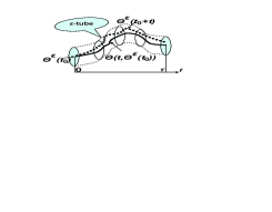
a) b)

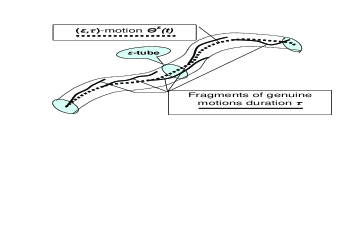
Figure 12: An $(\varepsilon,\tau)$-motion $\Theta^{\varepsilon}(t_{0}+t)$ ($t\in[0,\tau]$) in the $\varepsilon$-tube near a genuine motion $\Theta(t,\Theta^{\varepsilon}(t_{0}))$ ($t\in[0,\tau]$) duration $\tau$ (a), and an $(\varepsilon,\tau)$-motion $\Theta^{\varepsilon}(t)$ with fragments of genuine motions duration $\tau$ in the $\varepsilon$-tube near $\Theta^{\varepsilon}(t)$ (b).

It is convenient to introduce individual $\varepsilon$-motions. A function of time $\Theta^{\varepsilon}(t)$ with values in $X$, defined at $t\geq 0$, is called $(\varepsilon,x)$-motion $(\varepsilon>0)$, if $\Theta^{\varepsilon}(0)=x$ and for any $t_{0}\geq 0$, $t\in[0,\tau]$ the inequality $\rho(\Theta^{\varepsilon}(t_{0}+t),\Theta(t,\Theta^{\varepsilon}(t_{0})))<\varepsilon$ holds. In other words, if for an arbitrary point $\Theta^{\varepsilon}(t_{0})$ one considers its motion due to phase flow of dynamical system, this motion will diverge $\Theta^{\varepsilon}(t_{0}+t)$ from no more than at $\varepsilon$ for $t\in[0,\tau]$. Here $[0,\tau]$ is a certain interval of time, its length $\tau$ is not very important (it is important that it is fixed), because later we shall consider the case $\varepsilon\rightarrow 0$. For a given $\tau$ we shall call the $(\varepsilon,x)$-motion $(\varepsilon,x,\tau)$-motion when reference to $\tau$ is necessary. On any interval $[t_{0},t_{0}+\tau]$ an $(\varepsilon,x,\tau)$-motion deviates from a genuine motion not further than on distance $\varepsilon$ if these motions coincide at time moment $t_{0}$ (Fig. 12a). If a genuine motion starts from a point of an $(\varepsilon,x,\tau)$-trajectory, it remains in the $\varepsilon$-tube near that $(\varepsilon,\tau)$-motion during time $\tau$ (Fig. 12b).

Limit sets of $\varepsilon$-motions

Let us study the limit behaviour of the coarse-grained trajectories ${\bf\Theta}_{t}^{\varepsilon}A$, and than take the limit $\varepsilon\to 0$. For systems with complicated dynamics, this limit may differ significantly from the limit behaviour of the original system for $\varepsilon=0$. This effect of the perturbation influence in the zero limit is a “smile of a Cheshire cat:” the cat tends to disappear, leaving only its smile hanging in the air.

For any $\Theta^{\varepsilon}(t)$ the $\omega$-limit set $\omega(\Theta^{\varepsilon})$ is the set of all limit points of $\Theta^{\varepsilon}(t)$ at $t\to\infty$. For any $x\in X$ a set $\omega^{\varepsilon}(x)$ is a totality of all $\omega$-limit points of all $(\varepsilon,x)$-motions:

$$\omega^{\varepsilon}(x)=\bigcup_{\Theta^{\varepsilon}(0)=x}\omega(\Theta^{\varepsilon}).$$

For $\varepsilon\to 0$ we obtain the set

$$\omega^{0}(x)=\bigcap_{\varepsilon>0}\omega^{\varepsilon}(x).$$

Firstly, it is necessary to notice that $\omega^{\varepsilon}(x)$ does not always tend to $\omega(x)$ as $\varepsilon\to 0$: the set $\omega^{0}(x)$ may not coincide with $\omega(x,k)$.

The sets $\omega^{0}(x)$ are closed and invariant. Let $x\in\omega^{0}(x)$. Then for any $\varepsilon>0$ there exists periodical $(\varepsilon,x)$-motion (This is a version of Anosov’s $C^{0}$-closing lemma [53] ; Katok2 ).

The function $\omega^{0}(x)$ is upper semicontinuous. It means that for any sequence $x_{i}\to x$ all limit points of all sequences $y_{i}\in\omega^{0}(x_{i})$ belong to $\omega^{0}(x)$.

In order to study the limit behaviour for all initial conditions, let us join all $\omega^{0}(x)$:

$$\omega^{0}=\bigcup_{x\in X}\omega^{0}(x)=\bigcup_{x\in X}\bigcap_{\varepsilon>0}\omega^{\varepsilon}(x)=\bigcap_{\varepsilon>0}\bigcup_{x\in X}\omega^{\varepsilon}(x).$$ (121)

The set $\omega^{0}$ is closed and invariant. If $y\in\omega^{0}$ then $y\in\omega^{0}(y)$. If $Q\subset\omega^{0}$ and $Q$ is connected, then $Q\subset\omega^{0}(y)$ for any $y\in Q$.

The $\varepsilon$-motions were studied earlier in differential dynamics, in connection with the theory of Anosov about $\varepsilon$-trajectories and its applications [53] ; [54] ; [55] ; [57] ; sinai . For systems with hyperbolic attractors an important $\varepsilon$-motion shadowing property was discovered: for a given $\eta>0$ and sufficiently small $\varepsilon>0$ for any $\varepsilon$-motion $\Theta^{\varepsilon}(t)$ there exists a motion of the non-perturbed system $\Theta(t,x)$ that belongs to $\eta$ - neighborhood of $\Theta^{\varepsilon}(t)$:

$$\rho(\Theta^{\varepsilon}(\phi(t)),\Theta(t,x))<\eta,$$

for $t>0$ and some monotonous transformation of time $\phi(t)$ ($t-\phi(t)=O(\varepsilon t)$). The sufficiently small coarse-graining changes nothing in dynamics of systems with this shadowing property, because any $\varepsilon$-motion could be approximated uniformly by genuine motions on the whole semiaxis $t\in[0,\infty[$.

Preorder and equivalence generated by dynamics

Let $x_{1},x_{2}\in X$. Let us say $x_{1}\succsim_{\Theta}x_{2}$ if for any $\varepsilon>0$ there exists such a $(\varepsilon,x_{1})$-motion $\Theta^{\varepsilon}(t)$ ($\Theta^{\varepsilon}(0)=x_{1}$) that $\Theta^{\varepsilon}(t_{0})=x_{2}$ for some $t_{0}\geq 0$.

Let $x_{1},x_{2}\in X$. Say that points $x_{1}$ and $x_{2}$ are $\Theta$-equivalent (denotation $x_{1}\sim_{\Theta}x_{2}$), if $x_{1}\succsim_{\Theta}x_{2}$ and $x_{2}\succsim_{\Theta}x_{1}$.

The relation $\succsim_{\Theta}$ is a closed $\Theta$-invariant preorder relation on $X$:

• It is reflexive: $x\succsim_{\Theta}x$ for all $x\in X$;

• It is transitive: $x_{1}\succsim_{\Theta}x_{2}$ and $x_{2}\succsim_{\Theta}x_{3}$ implies $x_{1}\succsim_{\Theta}x_{3}$;

• The set of pairs $(x_{1},x_{2})$, for which $x_{1}\sim_{\Theta}x_{2}$ is closed in $X$;

• If $x_{1}\succsim_{\Theta}x_{2}$ then $\Theta(t,x_{1})\succsim_{\Theta}\Theta(t,x_{2})$ for any $t>0$.

The necessary and sufficient conditions for the preorder $\succsim_{\Theta}$ relation are as follows: $x_{1}\succsim_{\Theta}x_{2}$ if and only if either $x_{2}\in\omega^{0}(x_{1})$ or $x_{2}=\Theta(t,x_{1})$ for some $t\geq 0$. Therefore,

$$\omega^{0}(x)=\{y\in\omega^{0}\ |\ x\succsim_{\Theta}y\}$$ (122)

The relation $\sim_{\Theta}$ is a closed $\Theta$-invariant equivalence relation:

• The set of pairs $(x_{1},x_{2})$, for which $x_{1}\sim_{\Theta}x_{2}$ is closed in $X$;

• If $x_{1}\sim x_{2}$ and $x_{1}\neq x_{2}$, then $x_{1}$- and $x_{2}$-motions are whole and $\sim_{\Theta}\Theta(t,x_{2})$ for any $t\in]-\infty,\infty[\ \Theta(t,x_{1})$.

If $x_{1}\neq x_{2}$, then $x_{1}\sim_{\Theta}x_{2}$ if and only if $\omega^{0}(x_{1})=\omega^{0}(x_{2})$ , $x_{1}\in\omega^{0}(x_{1})$, and $x_{2}\in\omega^{0}(x_{2})$.

Compare with [52] , where analogous theorems are proved for relations defined by action functional for randomly perturbed dynamics.

The coarsened phase portrait

We present the results about the coarsened phase portrait as a series of theorems.

Let us remind, that topological space is called totally disconnected if there exist a base of topology, consisting of sets which are simultaneously open and closed. Simple examples of such spaces are discrete space and Cantor’s discontinuum. In a totally disconnected space all subsets with more than one element are disconnected. Due to the following theorem, in the coarsened phase portrait we have a totally disconnected space instead of finite set of attractors mentioned in the naive dream of applied dynamics.

Theorem 4.1

The quotient space $\omega^{0}/\sim_{\Theta}$ is compact and totally disconnected.

The space $\omega^{0}/\sim_{\Theta}$ with the factor-relation $\succsim_{\Theta}$ on it is the generalized Smale diagram with the generalized Smale order on it Diss ; SloRelMono .

Attractors and basins of attraction are the most important parts of a phase portrait. Because of (122), all attractors are saturated downwards. The set $Y\subset\omega^{0}$ is saturated downwards, if for any $y\in Y$,

$$\{x\in\omega^{0}\ |\ y\succsim_{\Theta}x\}\subset Y.$$

Every saturated downwards subset in $\omega^{0}$ is saturated also for the equivalence relation $\sim_{\Theta}$ and includes with any $x$ all equivalent points. The following theorem states that coarsened attractors $Y$ (open in $\omega^{0}$ saturated downwards subsets of $\omega^{0}$) have open coarsened basins of attraction $\mathcal{B}^{0}(Y)$.

Theorem 4.2

Let $Y\subset\omega^{0}$ be open (in $\omega^{0}$) saturated downwards set. Then the set $\mathcal{B}^{0}(Y)=\{x\in X\ |\ \omega^{0}(x)\subset Y\}$ is open in $X$.

There is a natural expectation that $\omega$-limit sets can change by jumps on boundaries of basins of attraction only. For the coarsened phase portrait it is true.

Theorem 4.3

The set $B$ of all points of discontinuity of the function $\omega^{0}(x)$ is the subset of first category in $X$. If $x\in B$ then $\Theta(t,x)\in B$ for all $t$ when $\Theta(t,x)$ is defined.

Theorem 4.4

Let $x\in X$ be a point of discontinuity of the function $\omega^{0}(x)$. Then there is such open in $\omega^{0}$ saturated downwards set $W$ that $x\in\partial\mathcal{B}^{0}(W)$.

The function $\omega^{0}(x)$ is upper semicontinuous, hence, in any point $x^{*}$ of its discontinuity the lower semicontinuity is broken: there exist a point $y^{*}\in\omega^{0}(x^{*})$, a number $\eta>0$, and a sequence $x_{i}\to x^{*}$ such that

$$\rho(y^{*},y)>\eta\;\mbox{for any}\;y\in\omega^{0}(x_{i})\;\mbox{and all}\;i.$$

The classical Smale order for hyperbolic systems was defined on a finite totality $A_{1},\ldots A_{n}$ of basic sets that are closed, invariant, and transitive (i.e. containing a dense orbit). $A_{i}\succ A_{j}$ if there exists such $x\in X$ that $x$-trajectory is whole, $\alpha(x)\subset A_{i}$, $\omega(x)\subset A_{j}$. Such special trajectories exist in the general case of coarsened dynamical system also.

Theorem 4.5

Let $X$ be connected, $\omega^{0}$ be disconnected. Then there is such $x\in X$ that $x$-motion is whole and $x\not\in\omega^{0}$. There is also such partition of $\omega^{0}$ that

$$\omega^{0}=W_{1}\cup W_{2},\ W\cap W_{2}=\varnothing,\ \alpha_{f}(x)\subset W_{1},\ \omega^{0}(x)\subset W_{2},$$

and $W_{1,2}$ are open and, at the same time, closed subsets of $\omega^{0}$ (it means that $W_{1,2}$ are preimages of open–closed subsets of the quotient space $\omega^{0}/\sim_{\Theta}$).

This theorem can be applied, by descent, to connected closures of coarsened basins of attraction $\mathcal{B}^{0}(Y)$ (see Theorem 4.2).

Theorems 4.1–4.5 give us the picture of coarsened phase portrait of a general dynamical system, and this portrait is qualitatively close to phase portraits of structurally stable systems: rough 2D systems, the Morse–Smale systems and the hyperbolic Smale systems. For proofs and some applications we address to Diss ; SloRelMono .

Stability of the coarsened phase portrait under smooth perturbations of vector fields

In order to analyze stability of this picture under the perturbation of the vector field (or the diffeomorphism, for discrete time dynamics) it is necessary to introduce $C^{k}$ $\varepsilon$-fattening in the space of smooth vector fields instead of periodic $\varepsilon$-fattening of phase points. We shall discuss a $C^{k}$-smooth dynamical system $\Theta$ on a compact $C^{m}$-manifold $M(0\leq k\leq m)$. Let $\Theta_{t}$ be the semigroup of phase flow transformations (shifts in time $t\geq 0$) and $U_{\varepsilon}(\Theta)$ be the set of phase flows that corresponds to a closed $\varepsilon$-neighborhood of system $\Theta_{t}$ in the $C^{k}$-norm topology of vector fields. The positive semi-trajectory of phase point $x$ is a set $\Theta(x)=\{\Theta_{t}(x)\colon t\geq 0\}$. The $C^{k}$ $\varepsilon$-fattened semi-trajectory is $\Theta^{\varepsilon}(x)=\bigcup_{\Phi\in U_{\varepsilon}(\Theta)}\Phi(x)$. Let us take this set with all limits for $t\rightarrow\infty$. It is the closure $\overline{\Theta^{\varepsilon}(x)}$. After that, let us take the limit $\varepsilon\rightarrow 0$: $P_{x}=\bigcap_{\varepsilon>0}\overline{\Theta^{\varepsilon}(x)}$ (it is an analogue of $\Theta(x)\cup\omega_{0}(x)$ from our previous consideration for general dynamical systems). Following [69] let us call this set $P_{x}$ a prolongation of the semi-trajectory $\Theta(x)$.

A trajectory of a dynamical system is said to be stable under $C^{k}$ constantly-acting perturbations if its prolongation is equal to its closure: $P_{x}=\overline{\Theta(x)}$

For a given dynamical system let $L(\Theta)$ denote the union of all trajectories that are stable in the above sense and let $\mathbb{L}_{1}$ be the set of all dynamical systems $\Theta$ for which $L(\Theta)$ is dense in phase space: $\overline{L(\Theta)}=M$. All structurally stable systems belong to $\mathbb{L}_{1}$. The main result of [69] is as follows:

Theorem 4.6

The set $\mathbb{L}_{1}$ is a dense $\mathbb{G_{\delta}}$ in the space of $C^{k}$ dynamical systems with the $C^{k}$ norm.

So, for almost all smooth dynamical systems almost all trajectories are stable under smooth constantly-acting perturbations: this type of stability is typical.

5 Conclusion

Two basic ideas of coarse-graining are presented. In the Ehrenfests’ inspired approach the dynamics of distributions with averaging is studied. In the metric approach the starting point of analysis is dynamics of sets with periodical $\varepsilon$-fattening.

The main question of the Ehrenfests’ coarse-graining is: where should we take the coarse-graining time $\tau$? There are two limit cases: $\tau\to 0$ and $\tau\to\infty$ (physically, $\infty$ here means the time that exceeds all microscopic time scales). The first limit, $\tau\to 0$, returns us to the quasi-equilibrium approximation. The second limit is, in some sense, exact (if it exists). Some preliminary steps in the study of this limit are made in GKGeoNeo ; Plenka ; GorKar . On this way, the question about proper values of the Prandtl number, as well, as many other similar questions about kinetic coefficients, has to be solved.

The constructed family of chains between conservative (with the Karlin–Succi involution) and maximally dissipative (with Ehrenfests’ projection) ones give us a possibility to model hydrodynamic systems with various dissipation (viscosity) coefficients that are decoupled with time steps. The collision integral is successfully substituted by combinations of the involution and projection.

The direct descendant of the Ehrenfests’ coarse-graining, the kinetic approach to filtering of continuum equations, seems to be promising and physically reasonable: if we need to include the small eddies energy into internal energy, let us lift the continuum mechanics to kinetics where all the energies live together, make there the necessary filtering, and then come back. Two main questions: when the obtained filtered continuum mechanics is stable, and when there is way back from filtered kinetics to continuum mechanics, have unexpectedly the similar answer: the filter width $\Delta$ should be proportional to the square root of the Knudsen number. The coefficient of this proportionality is calculated from the entropic stability conditions.

The metric coarse-graining by $\varepsilon$-motions in the limit $\varepsilon\to 0$ gives the stable picture with the totally disconnected system of basic sets that form sources and sinks structure in the phase space. Everything looks nice, but now we need algorithms for effective computation and representation of the coarsened phase portrait even in modest dimensions 3-5 (for discrete time systems in dimensions 2-4).

It is necessary to build a bridge between theoretical topological picture and applied computations. In some sense, it is the main problem of modern theory of dynamical systems to develop language and tools for constructive analysis of arbitrary dynamics. Of course, the pure topological point of view is unsufficient, and we need an interplay between measure and topology of dynamical systems, perhaps, with inclusion of some physical and probabilistic ideas.

- (1) P. Ehrenfest, T. Ehrenfest-Afanasyeva, The Conceptual Foundations of the Statistical Approach in Mechanics, In: Mechanics Enziklopädie der Mathematischen Wissenschaften, Vol. 4., Leipzig, 1911. (Reprinted: P. Ehrenfest, T. Ehrenfest-Afanasyeva, The Conceptual Foundations of the Statistical Approach in Mechanics, Dover Phoneix, 2002.)
- (2) H. Grabert, Projection operator techniques in nonequilibrium statistical mechanics, Springer Verlag, Berlin, 1982.
- (3) A.N. Gorban, I.V. Karlin, A.Yu. Zinovyev, Constructive methods of invariant manifolds for kinetic problems, Phys. Reports 396, 4-6 (2004), 197–403. Preprint online: http://arxiv.org/abs/cond-mat/0311017.
- (4) A.N. Gorban, I.V. Karlin, Invariant manifolds for physical and chemical kinetics, Lect. Notes Phys., Vol. 660, Springer, Berlin, Heidelberg, New York, 2005.
- (5) A.N. Gorban, I.V. Karlin, P. Ilg, and H.C. Öttinger, Corrections and enhancements of quasi–equilibrium states, J. Non–Newtonian Fluid Mech. 96 (2001), 203–219.
- (6) K.G. Wilson, and J. Kogut. The renormalization group and the -expansion, Phys. Reports 12C (1974), 75-200.
- (7) O. Pashko, Y. Oono, The Boltzmann equation is a renormalization group equation, Int. J. Mod. Phys. B 14 (2000), 555–561.
- (8) Y. Hatta, T. Kunihiro, Renormalization group method applied to kinetic equations: roles of initial values and time, Annals Phys. 298 (2002), 24–57.
- (9) I.G. Kevrekidis, C.W. Gear, J.M. Hyman, P.G. Kevrekidis, O. Runborg, C. Theodoropoulos, Equation-free, coarse-grained multiscale computation: enabling microscopic simulators to perform system-level analysis, Comm. Math. Sci. 1 4 (2003), 715–762.
- (10) A.J. Chorin, O.H. Hald, R. Kupferman, Optimal prediction with memory, Physica D 166 (2002), 239–257.
- (11) A.N. Gorban, I.V. Karlin, H.C. Öttinger, and L.L. Tatarinova, Ehrenfests’ argument extended to a formalism of nonequilibrium thermodynamics, Phys.Rev.E 63 (2001), 066124.
- (12) A.N. Gorban, I.V. Karlin, Uniqueness of thermodynamic projector and kinetic basis of molecular individualism, Physica A 336, 3-4 (2004), 391–432.
- (13) J. Leray, Sur les movements d un fluide visqueux remplaissant l espace, Acta Mathematica, 63 (1934), 193 -248.
- (14) J. Smagorinsky, General Circulation Experiments with the Primitive Equations: I. The Basic Equations, Mon. Weather Rev. 91 (1963), 99–164.
- (15) M. Germano, Turbulence: the filtering approach, J. Fluid Mech. 238 (1992), 325–336.
- (16) D. Carati, G.S. Winckelmans, H. Jeanmart, On the modelling of the subgrid-scale and filtered-scale stress tensors in large-eddy simulation, J. Fluid Mech., 441 (2001), 119–138.
- (17) M. Lesieur, O. Métais, P. Comte, Large-Eddy Simulations of Turbulence, Cambridge University Press, 2005.
- (18) S. Ansumali, I.V. Karlin, S. Succi, Kinetic Theory of Turbulence Modeling: Smallness Parameter, Scaling and Microscopic Derivation of Smagorinsky Model, Physica A, 338 (2004), 379–394.
- (19) S. Succi, The lattice Boltzmann equation for fluid dynamics and beyond, Clarendon Press, Oxford, 2001.
- (20) S. Smale, Structurally stable systems are not dense, Amer. J. Math. 88 (1966), 491–496.
- (21) V.A. Dobrynskiĭ, A.N. Sharkovskiĭ, Genericity of the dynamical systems almost all orbits of which are stable under sustained perturbations, Soviet Math. Dokl. 14 (1973), 997–1000.
- (22) A.N. Gorban, Slow relaxations and bifurcations of omega-limit sets of dynamical systems, PhD Thesis in Physics & Math. (Differential Equations & Math.Phys), Kuibyshev, Russia, 1980.
- (23) A.N. Gorban, Singularities of Transition Processes in Dynamical Systems: Qualitative Theory of Critical Delays, Electronic Journal of Differential Equations, Monograph 05, 2004. http://ejde.math.txstate.edu/Monographs/05/abstr.html (Includes English translation of Diss .)
- (24) B.A. Huberman, W.F. Wolff, Finite precision and transient behavior, Phys. Rev. A 32, 6 (1985), 3768–3770.
- (25) C. Beck, G. Roepsorff, Effects of phase space discretization on the long–time behavior of dynamical systems, Physica D 25 (1987), 173–180.
- (26) C. Grebogi, E. Ott, J.A. Yorke, Roundoff–induced periodicity and the correlation dimension of chaotic attractors, Phys. Rev. A 38, 7 (1988), 3688–3692.
- (27) P. Diamond, P. Kloeden, A. Pokrovskii, A. Vladimirov, Collapsing effect in numerical simulation of a class of chaotic dynamical systems and random mappings with a single attracting centre, Physica D 86 (1995), 559–571.
- (28) L. Longa, E.M.F. Curado, A. Oliveira, Rounoff–induced coalescence of chaotic trajectories, Phys. Rev. E 54, 3 (1996), R2201–R2204.
- (29) P.-M. Binder, J.C. Idrobo, Invertibility of dynamical systems in granular phase space, Phys. Rev. E 58, 6 (1998), 7987–7989.
- (30) C. Dellago, Wm. G. Hoover, Finite–precision stationary states at and away from equilibrium, Phys. Rev. E 62, 5 (2000), 6275–6281.
- (31) B. Bollobas, Random Graphs (Cambridge Studies in Advanced Mathematics), Cambridge University Press, 2001.
- (32) M.I. Freidlin, A.D. Wentzell, Random Perturbations of Dynamical Systems (Grundlehren der mathematischen Wissenschaften, V.260), Springer-Verlag New York, Berlin, Heidelberg, 1998.
- (33) L. Arnold, Random Dynamical Systems, Springer Monographs in Mathematics, 16, Springer, Berlin, Heidelberg, New York, 2002.
- (34) A.N. Gorban, Equilibrium encircling. Equations of chemical kinetics and their thermodynamic analysis, Nauka, Novosibirsk, 1984.
- (35) A.N. Gorban, V.I. Bykov, G.S. Yablonskii, Essays on chemical relaxation, Nauka, Novosibirsk, 1986.
- (36) G.S.Yablonskii, V.I.Bykov, A.N. Gorban, and V.I.Elokhin, Kinetic Models of Catalytic Reactions (Series “Comprehensive Chemical Kinetics,” V.32, ed. by R.G. Compton), Elsevier, Amsterdam, 1991,
- (37) Y.B. Zeldovich, Proof of the Uniqueness of the Solution of the Equations of the Law of Mass Action, In: Selected Works of Yakov Borisovich Zeldovich, Vol. 1, J.P. Ostriker (Ed.), Princeton University Press, Princeton, USA, 1996, 144-148.
- (38) Bhatnagar, P.L., Gross, E.P., Krook, M., A model for collision processes in gases. I. Small amplitude processes in charged and neutral one–component systems, Phys. Rev., 94, 3 (1954), 511–525.
- (39) Gorban, A.N., Karlin, I.V., General approach to constructing models of the Boltzmann equation, Physica A, 206 (1994), 401–420.
- (40) D. Hilbert, Begründung der kinetischen Gastheorie, Math. Annalen 72 (1912), 562–577.
- (41) D. Ruelle, Smooth Dynamics and New Theoretical Ideas in Nonequilibrium Statistical Mechanics, J. Stat. Phys. 95 (1-2) (1999), 393-468.
- (42) S. Kullback, Information theory and statistics, Wiley, New York, 1959.
- (43) A.N. Gorban, I.V. Karlin, Family of additive entropy functions out of thermodynamic limit, Phys. Rev. E 67 (2003), 016104.
- (44) P. Gorban, Monotonically equivalent entropies and solution of additivity equation, Physica A 328 (2003), 380-390.
- (45) S. Abe, Y. Okamoto (Eds.), Nonextensive statistical mechanics and its applications, Springer, Heidelberg, 2001.
- (46) B.M. Boghosian, P.J. Love, P.V. Coveney, I.V. Karlin, S. Succi, J. Yepez, Galilean-invariant lattice-Boltzmann models with H theorem, Phys. Rev. E 68, 2 (2003), 025103(R)
- (47) G.W. Gibbs, Elementary Principles of Statistical Mechanics, Dover, 1960.
- (48) E.T. Jaynes, Information theory and statistical mechanics, in: Statistical Physics. Brandeis Lectures, V.3, K. W. Ford, ed., New York: Benjamin, 1963, pp. 160–185.
- (49) D. Zubarev, V. Morozov, G. Röpke, Statistical mechanics of nonequilibrium processes, Akademie Verlag, Berlin, V.1, 1996, V.2, 1997.
- (50) H. Grad, On the kinetic theory of rarefied gases, Comm. Pure and Appl. Math. 2 4, (1949), 331–407.
- (51) J.T. Alvarez-Romero, L.S. García-Colín, The foundations of informational statistical thermodynamics revisited, Physica A 232, 1-2 (1996), 207–228
- (52) R.E. Nettleton, E.S. Freidkin, Nonlinear reciprocity and the maximum entropy formalism, Physica A 158, 2 (1989), 672–690.
- (53) N.N. Orlov, L.I. Rozonoer, The macrodynamics of open systems and the variational principle of the local potential, J. Franklin Inst. 318 (1984), 283–314 and 315–347.
- (54) A.M. Kogan, L.I. Rozonoer, On the macroscopic description of kinetic processes, Dokl. AN SSSR 158, 3 (1964), 566–569.
- (55) A.M. Kogan, Derivation of Grad–type equations and study of their properties by the method of entropy maximization, Prikl. Matem. Mech. 29 (1) (1965), 122–133.
- (56) L.I. Rozonoer, Thermodynamics of nonequilibrium processes far from equilibrium, in: Thermodynamics and Kinetics of Biological Processes (Nauka, Moscow, 1980), 169–186.
- (57) J. Karkheck, G. Stell, Maximization of entropy, kinetic equations, and irreversible thermodynamics Phys. Rev. A 25, 6 (1984), 3302–3327.
- (58) N.N. Bugaenko, A.N. Gorban, I.V. Karlin, Universal Expansion of the Triplet Distribution Function, Teoret. i Matem. Fisika 88, 3 (1991), 430–441 (Transl.: Theoret. Math. Phys. (1992), 977–985).
- (59) A.N. Gorban, I.V. Karlin, Quasi–equilibrium approximation and non–standard expansions in the theory of the Boltzmann kinetic equation, in: ”Mathematical Modelling in Biology and Chemistry. New Approaches”, ed. R. G. Khlebopros, Nauka, Novosibirsk, P. 69–117 (1991).[in Russian]
- (60) A.N. Gorban, I.V. Karlin, Quasi–equilibrium closure hierarchies for the Boltzmann equation, Physica A 360, 2 (2006), 325–364. (Includes translation of the first part of MBCh ).
- (61) C.D. Levermore, Moment Closure Hierarchies for Kinetic Theories, J. Stat. Phys. 83 (1996), 1021–1065.
- (62) R. Balian, Y. Alhassid, H. Reinhardt, Dissipation in many–body systems: A geometric approach based on information theory, Phys. Reports 131, 1 (1986), 1–146.
- (63) P. Degond, C. Ringhofer, Quantum moment hydrodynamics and the entropy principle, J. Stat. Phys. 112 (2003), 587–627.
- (64) P. Ilg, I.V. Karlin, H.C. Öttinger, Canonical distribution functions in polymer dynamics: I. Dilute solutions of flexible polymers, Physica A 315 (2002), 367–385.
- (65) P. Ilg, I.V. Karlin, M. Kröger, H.C. Öttinger, Canonical distribution functions in polymer dynamics: II Liquid–crystalline polymers, Physica A 319 (2003), 134–150.
- (66) P. Ilg, M. Kröger, Magnetization dynamics, rheology, and an effective description of ferromagnetic units in dilute suspension, Phys. Rev. E 66 (2002) 021501. Erratum, Phys. Rev. E 67 (2003), 049901(E).
- (67) P. Ilg, I.V. Karlin, Combined micro–macro integration scheme from an invariance principle: application to ferrofluid dynamics, J. Non–Newtonian Fluid Mech. 120, 1-3 (2004), 33–40 2004. Ppeprint online: http://arxiv.org/abs/cond-mat/0401383.
- (68) B. Robertson, Equations of motion in nonequilibrium statistical mechanics, Phys. Rev. 144 (1966), 151–161.
- (69) P.J. Morrison, Hamiltonian description of the ideal fluid, Rev. Mod. Phys. 70 (1998), 467 -521.
- (70) E. Wigner, On the quantum correction for thermodynamic equilibrium, Phys. Rev. 40 (1932), 749–759.
- (71) A.O. Caldeira, A.J. Leggett, Influence of damping on quantum interference: An exactly soluble model, Phys. Rev. A 31 (1985), 1059–1066.
- (72) A.N. Gorban, I.V. Karlin, Reconstruction lemma and fluctuation–dissipation theorem, Revista Mexicana de Fisica 48, Supl. 1 (2002), 238–242.
- (73) A.N. Gorban, I.V. Karlin, Macroscopic dynamics through coarse–graining: A solvable example, Phys. Rev. E 56 (2002), 026116.
- (74) A.N. Gorban, I.V. Karlin, Geometry of irreversibility, in: Recent Developments in Mathematical and Experimental Physics, Vol. C, Ed. F. Uribe, Kluwer, Dordrecht, 2002, 19–43.
- (75) A.N. Gorban, I.V. Karlin, Geometry of irreversibility: The film of nonequilibrium states, Preprint IHES/P/03/57, Institut des Hautes Études Scientifiques in Bures-sur-Yvette (France), 2003. 69 p. Preprint on-line: http://arXiv.org/abs/cond-mat/0308331.
- (76) I.V. Karlin, L.L. Tatarinova, A.N. Gorban, H.C. Öttinger, Irreversibility in the short memory approximation, Physica A 327, 3-4 (2003), 399–424.
- (77) J.L. Lebowitz, Statistical Mechanics: A Selective Review of Two Central Issues, Rev. Mod. Phys. 71 (1999), S346.
- (78) S. Goldstein, J.L. Lebowitz, On the (Boltzmann) Entropy of Nonequilibrium Systems, Physica D 193 (2004), 53–66.
- (79) Chapman, S., Cowling, T., Mathematical theory of non-uniform gases, Third edition, Cambridge University Press, Cambridge, 1970.
- (80) C. Cercignani, The Boltzmann equation and its applications, Springer, New York, 1988.
- (81) L. Mieussens, H. Struchtrup, Numerical Comparison of Bhatnagar–Gross–Krook models with proper Prandtl number, Phys. Fluids 16, 4 (2004), 2797–2813.
- (82) R.M. Lewis, A unifying principle in statistical mechanics, J. Math. Phys. 8 (1967), 1448–1460.
- (83) Lyapunov A.M., The general problem of the stability of motion, Taylor & Francis, London, 1992.
- (84) L.B. Ryashko, E.E. Shnol, On exponentially attracting invariant manifolds of ODEs, Nonlinearity 16 (2003), 147–160.
- (85) C. Foias, M.S. Jolly, I.G. Kevrekidis, G.R. Sell, E.S. Titi, On the computation of inertial manifolds, Phys. Lett. A 131, 7–8 (1988), 433–436.
- (86) Y. Sone, Kinetic theory and fluid dynamics, Birkhäuser, Boston, 2002.
- (87) C.W. Gear, T.J. Kaper, I.G. Kevrekidis, A. Zagaris, Projecting to a slow manifold: singularly perturbed systems and legacy codes, SIAM J. Appl. Dynamical Systems 4, 3 (2005), 711–732.
- (88) F. Higuera, S. Succi, R. Benzi, Lattice gas-dynamics with enhanced collisions, Europhys. Lett. 9 (1989), 345–349.
- (89) I.V. Karlin, A.N. Gorban, S. Succi, V. Boffi, V. Maximum entropy principle for lattice kinetic equations, Phys. Rev. Lett. 81 (1998), 6–9.
- (90) H. Chen, S. Chen, W. Matthaeus, Recovery of the Navier–Stokes equation using a lattice–gas Boltzmann Method Phys. Rev. A 45 (1992), R5339–R5342.
- (91) Y.H. Qian, D. d’Humieres, P. Lallemand, Lattice BGK models for Navier–Stokes equation, Europhys. Lett. 17, (1992), 479–484.
- (92) S. Succi, I.V. Karlin, H. Chen, Role of the theorem in lattice Boltzmann hydrodynamic simulations, Rev. Mod. Phys. 74 (2002), 1203–1220.
- (93) I.V. Karlin, A. Ferrante, H.C. Öttinger, Perfect entropy functions of the Lattice Boltzmann method, Europhys. Lett. 47, 182–188 (1999).
- (94) S. Ansumali, I.V. Karlin, Entropy function approach to the lattice Boltzmann method, J. Stat. Phys. 107 291–308 (2002).
- (95) R. Cools, An encyclopaedia of cubature formulas, J. of Complexity, Volume 19, Issue 3, June 2003, Pages 445-453.
- (96) A. Gorban, B. Kaganovich, S. Filippov, A. Keiko, V. Shamansky, I. Shirkalin, Thermodynamic Equilibria and Extrema: Analysis of Attainability Regions and Partial Equilibrium, Springer, Berlin, Heidelberg, New York, 2006 (in press).
- (97) Ansumali, S., Karlin, I.V., Kinetic Boundary condition for the lattice Boltzmann method, Phys. Rev. E, 66 (2002), 026311.
- (98) J.R. Higgins, Sampling Theory in Fourier and Signal Analysis: Foundations, Clarendon, Oxford, 1996.
- (99) J.R. Higgins, R.L. Stens, Sampling Theory in Fourier and Signal Analysis: Advanced Topics, Clarendon, Oxford, 1999.
- (100) J.G.M. Kuerten, B.J. Geurts, A.W. Vreman, M. Germano. Dynamic inverse modeling and its testing in large-eddy simulations of the mixing layer. Phys. Fluids, 11: 3778-3785, 1999.
- (101) A.W. Vreman, The adjoint filter operator in large-eddy simulation of turbulent flow, Phys. Fluids, 16 (2004), 2012–2022
- (102) B.J. Geurts, D.D. Holm, Nonlinear regularization for large-eddy simulation, Phys. Fluids, 15, 1 (2003), L13–L16.
- (103) P. Moeleker, A. Leonard, Lagrangian methods for the tensor-diffusivity subgrid model, J. Comp. Phys., 167 (2001), 1–21.
- (104) G. Berkooz, P. Holmes, J.L. Lumley, The proper orthogonal decomposition in the analysis of turbulent flows, Annual Rev. Fluid Mech., 25 (1993), 539–575.
- (105) I.T. Jolliffe, Principal component analysis, Springer–Verlag, 1986.
- (106) K. Kunisch, S. Volkwein, Galerkin Proper Orthogonal Decomposition Methods for a General Equation in Fluid Dynamics, SIAM J Numer. Anal. 40, 2 (2002), 492- 515.
- (107) M. Marion, R. Temam, Nonlinear Galerkin methods, SIAM J. Numer. Anal., 26 (1989), 1139–1157.
- (108) A. Gorban, A. Zinovyev, Elastic Principal Graphs and Manifolds and their Practical Applications, Computing 75, 359 379 (2005),
- (109) G.D. Birkhoff, Dynamical systems, AMS Colloquium Publications, Providence, 1927. Online: http://www.ams.org/online _bks/coll9/
- (110) B. Hasselblatt, A. Katok, (Eds.), Handbook of Dynamical Systems, Elsevier, 2002.
- (111) A. Katok, B. Hasselblat, Introduction to the Modern Theory of Dynamical Systems, Encyclopedia of Math. and its Applications, Vol. 54, Cambridge University Press, 1995.
- (112) J. Milnor, On the concept of attractor, Comm. Math. Phys. 99, (1985), 177–195
- (113) P. Ashwin and J.R. Terry. On riddling and weak attractors. Physica D 142 (2000), 87–100.
- (114) D.V. Anosov, About one class of invariant sets of smooth dynamical systems, Proceedings of International conference on non-linear oscillation, V.2. Kiev, 1970, 39–45.
- (115) P. Walters, On the pseudoorbit tracing property and its relationship to stability, Lect. Notes Math. V. 668 (1978), 231–244.
- (116) J.E. Franke, J.F. Selgrade, Hyperbolicity and chain recurrence, J. Different. Equat. 26, 1 (1977), 27–36.
- (117) H. Easton, Chain transitivity and the domain of influence of an invariant set, Lect. Notes Math., V.668 (1978), p.95–102.
- (118) Y. Sinai, Gibbs measures in ergodic theory, Russ. Math. Surveys 166 (1972), pp. 21–69.
- (119) I.G. Malkin, On the stability under uniformly influencing perturbations, Prikl. Matem. Mech. 8, 3 (1944), 241–245.
- (120) V.E. Germaidze, N.N. Krasovskii, On the stability under sustained perturbations, Prikl. Matem. Mech. 21, 6 (1957), 769–775.
- (121) I.G. Malkin, The motion stability theory. Moscow: Nauka, 1966.
- (122) A. Strauss, A.J. Yorke, Identifying perturbations which preserved asymptotic stability, Proc. Amer. Math. Soc. 22, 2 (1969), 513–518.
- (123) M. Gromov, Metric structures for Riemannian and non-Riemannian spaces. Progress in Mathematics, 152. Birkhauser Boston, Inc., Boston, MA, 1999.