Elliptical invariance of distributions of the power type: the stability and extensivity issues
Abstract
In this paper we delve into some important properties of probability distributions of the power type in order to provide some answers to questions recently raised in the literature. More precisely, we focus on the properties of maximizers of generalized information measures and give results about their stability under addition-composition processes.
pacs:
PACS: 05.40.-a, 05.20.GgKeywords: power-law probabilistic distributions, superstatistics, stability, extensivity
1 Introduction
Non-logarithmic information measures have become vary fashionable nowadays, with multiple applications to different scientific disciplines (see, for instance, [1] and references therein). They were introduced in the cybernetic-information communities by Harvda-Charvat [2] in 1967 and Vadja [3] in 1968, and rediscovered by Daroczy in 1970 [4] with several echoes mostly in the field of image processing: see [5] for a historic summary and the pertinent references. In astronomy, physics, economics, biology etc…, these non-logarithmic information measures are often used under the form of the entropies as introduced by Tsallis since 1988 [6]. These entropies are maximized by power-type distributions. The properties of both discrete and continuous power-type distributions have been carefully reviewed recently in Ref. [7] in what respects to
-
1.
their behavior by convolution and
-
2.
their relationships with stable Lévy distributions.
In this paper, we wish to focus attention more closely on further properties of these distributions, and answer some open questions as raised in [7]; this way, we hope, in the wake of Refs. [8, 9, 10], to positively contribute to a more complete understanding of the ensuing theoretical context.
2 Definitions and Notations
In what follows we consider some probability density that maximize a generalized entropy, either of the Harvda-Charvat-Rényi type
| (1) |
or of the Tsallis type
| (2) |
where is a real parameter (called ”nonextensivity parameter" in [1]). As can be expressed as an increasing function of , both entropies have the same maximizers. As a consequence, all results expressed in this paper hold for both types of entropies, except in Section 6 that deals with a special property of . To each density , we associate its so-called escort distribution [11] defined as
Note that the dependence of on is not explicitly stated for notational simplicity.
2.1 Power-law distributions as entropy-maximizers
The following theorem generalizes to the variate case the characterization given in Ref. [7, Eq. (42)] for the maximum entropy distributions with fixed covariance.
Theorem 1
Under the q-covariance constraint
(where the covariance matrix is symmetric definite positive) and the normalization constraint , the power-law entropy (1) or (2) has a single maximizer equal to:
if
(3)
with
if
(4)
with
and with notation .
In the case we recover the results of [7, eq. (42)], namely
-
•
if
| (5) |
2.2 Student-t and Student-r distributions
In statistics, distribution (3) is called an variate Student-t with degrees of freedom and covariance matrix : it will be denoted as in the following. We notice that its nonextensivity parameter is linked to the dimension and the number of degrees of freedom by
Moreover, convergence of both integrals and requires the same condition, namely or equivalently In the next section, we will endow parameter with a meaning.
Accordingly, distribution (4) is an variate Student-r with degrees of freedom and covariance matrix : it will be denoted as We remark that its nonextensivity parameter is linked to parameter and dimension as
2.3 Stochastic representations
Beck and Cohen [11] have recently introduced in the literature an interesting statistical concept, baptized with the name superstatistics, that links different types of probability densities. In this vein, our distributions above can be shown to correspond to multivariate Gaussian densities whose covariance matrix fluctuates according to a certain law, as detailed in the two following theorems.
Theorem 2
If follows a distribution then a stochastic representation of writes 111in the following, sign means “is distributed as”
| (7) |
where is an variate Gaussian vector with unit covariance matrix, is a random variable independent of that follows a distribution222a chi distribution is ; chi distributions are restricted to integer degrees of freedom. If then the distribution should be extended to the distribution of the square-root of a gamma random variable with shape parameter equal to . For the sake of simplicity, we will speak of distribution in this case too. with number of degrees of freedom and
A remarkable fact deserves here emphasizing upon: this approach can be extended to the case when , with a noticeable difference. This extension is based on the following duality result.
Theorem 3
if and then random vector defined as
| (8) |
is such that with
If and denote the respective nonextensivity indices of and then
| (9) |
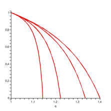
In Figure 1 below, values of as a function of are plotted for and (right to left). We remark that transformation (8) induces a one-to-one relationship between and and has the Gaussian distribution () as fixed point.
An important consequence of the above is the following dual result of theorem (2).
Theorem 4
If follows a distribution then a stochastic representation of writes
| (10) |
where is an variate Gaussian vector with unit covariance matrix, where and is a random variable independent of that follows a distribution with degrees of freedom.
Here, the important difference, as compared to the case , is to be found in the fact that the fluctuations, represented by the denominator of (10), are now dependent of the values of the Gaussian system through the presence of term .
2.4 Covariance matrices
The covariance matrices of both distributions are related to their covariance matrices as follows.
Theorem 5
Distribution has covariance matrix
| (11) |
provided that is . For example, a finite covariance matrix exists in the case only if
Theorem 6
Distribution has covariance matrix
| (12) |
2.5 Geometric characterization
Geometric characterizations of both distributions (3) and (4) in terms of projections of the uniform distribution on the sphere in are detailed in [14]. According to the stochastic representation (10), can be interpreted, if , as the marginal vector of a variate random vector uniformly distributed on the sphere in A link between this observation and the role of extended information measures in the microcanonical framework can be found in [14].
3 The stability issue
As noted in [7], distributions (3)
and (4) are not stable by convolution since they
do not belong to the Lévy class: the sum of two independent random
variables following either distribution
(3) or distribution (4) does
not follow any of these distributions again, as opposed to the
Maxwellian-Gaussian case. It is then suggested in [7]
that, in order to recover the original distribution after
summation, a certain kind of dependence should be
introduced between the components of the sum.
It is the aim of the next paragraph to show that such dependence can be accurately characterized
in the case of power-law distributions.
3.1 A first example: case
Let us assume, for instance, that and choose to be a random vector of dimension distributed according to (3). We extract from it two scalar components, say and ; according to (7), these two components can be expressed as
| (13) |
where denotes the first vector component.
Distribution of the components
We first remark from stochastic representation (13) that and are again distributed according to a Student-t distribution with dimension ; moreover, the extraction of components keeps the fluctuation variable unchanged, so that both and have unchanged number of degrees of freedom . Both have thus a new nonextensivity parameter that verifies
or equivalently
| (14) |
Moreover, it is easy to check that their respective variances are and , the two first diagonal entries of covariance matrix . The three curves in Figure 2 represent as a function of for and (from right to left).
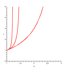
We note that
-
•
, since any component of a Gaussian vector is Gaussian
-
•
the nonextensivity parameter of a single component is larger than the nonextensivity parameter of the system it is extracted from
-
•
moreover, is all the larger since the dimension is large.
Distribution of the convolution The distribution of a linear combination of and can be computed as
| (15) | |||
| (16) |
so that is again distributed as a Student-t distribution with same parameter and variance We underline the fact that stability under convolution originates from the special type of dependence that exists between the components and namely from the fact that they belong to a same (larger) system: in more physical terms, and are components that have experienced the same random source of fluctuations.
3.2 A second example: case
We assume now that we extract two components and from a vector Then a stochastic representation of and is
so that (resp. ) follows a distribution with (resp. ) and its new index of nonextensivity verifies
or
| (17) |
We remark that (17) coincides with (14) since conservation of degrees of freedom in the Student-t case and in the Student-r case is expressed by the same condition.
In Figure 3 below, is represented as a function of for and (bottom to top).
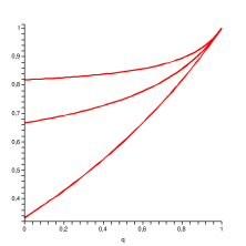
The same conclusions as in the case hold, namely:
-
•
if then (Gaussian case)
-
•
the nonextensivity parameter of an extracted component is always larger than the nonextensivity parameter of the original system; it is all the larger since the dimension is large
The distribution of a linear combination can be evaluated as
| (18) | |||
| (19) |
so that
3.3 Orthogonal invariance
These results can be generalized using the notion of elliptical distribution [13].
Definition 7
A distribution is elliptical (or elliptically invariant) if it writes
for some positive definite matrix called the characteristic matrix of and some function that may depend of
From (3) and (4), we check immediately that Student-t and Student-r distributions are elliptically invariant. This special property can be justified as follows: up to application of the mapping or , it may be assumed in (3) and (4) that or this special case of elliptical invariance is called spherical invariance. An equivalent definition of spherical invariance reads as follows: for all orthogonal matrices the distribution of coincides with the distribution of :
Now, the or entropy remains unchanged by orthogonal transformation since, for example
| (20) | |||
| (21) |
where we have used the fact that for any orthogonal matrix, Moreover, the constraints under which the entropy is maximized, that is
are themselves spherically invariant as well. Thus, it is not surprising that the maximizer of under these constraints is spherically invariant - and elliptically invariant in the more general case .
3.4 Properties of elliptical distributions and consequences
The stability property exposed in parts 3.1 and 3.2 appears as a particular case of the more general property of elliptical distributions that we cast here as follows:
Theorem 8
[13] If is distributed according to an elliptical distribution
and if is a full-rank matrix with then is again elliptically invariant with characteristic matrix
| (22) |
As a consequence, one can characterize the precise way in which power-law random vectors behave under linear transformation as follows.
Case of components’ extraction Suppose we extract the first components from a vector of the power-law type . This process corresponds to applying the matrix
to vector , and we conclude that where coincides with the principal block of and , corresponding to a new index of extensivity
| (23) |
For a power law vector , as remarked in part 3.2, conservation of the number of degrees of freedom yields the same condition as conservation of the number of degrees of freedom in the Student-t case, that is
or
| (24) |
In both (23) and (24), in (24), yielding the classical property of Boltzmann systems, any subsystem of which is still of the Boltzmann type.
Case of convolution Choosing in (22) yields the following results:
We note again that this stability result requires a special type of dependence between the components or namely the fact that they are extracted from the same system.
4 The stability issue for independent vectors
Few results exist about the convolution of two independent Student-t or Student-r vectors. In Ref. [16], Oliveira et al. remark that if and are independent and distributed, their sum
can be very accurately approximated as a for some depending on However, they provide only an approximation to the map
An important result can be stated when in the special case for which the number of degrees of freedom is an odd integer
Theorem 9
[8] If and are two independent vectors following a distribution and if is such that and , then the distribution of
can be expressed as
| (25) |
with
Since coefficients are positive and sum to (see [8] for a proof), this result can be interpreted as follows: the convolution of distributions with odd degrees of freedom follows a distribution whose degrees of freedom are randomized:
| (26) |
where is a random variable defined as
As an example, if and , we have
with
We note that conditions and are not restrictive since
-
•
if , then by parity of ,
-
•
if , then
An important result is the following one: formula (25) can be extended to the case where and provided and have the same covariance matrix : in that case, and have identity covariance, so that the distribution of can be computed using formula (25) and distribution of can be obtained by a simple change of variable.
5 Another approach to the stability issue: random convolution
A radically different approach to the problem we are discussing here, namely, the conditions of stability for power-type distributions, can be followed in the case by considering the polar factorization property of the stochastic representation (10).
Theorem 10
If has stochastic representation
where is a Gaussian vector with unit covariance matrix and is distributed, independent of , then is independent of ; we remark that the later is chi distributed with degrees of freedom.
An important consequence of this property is that it allows to derive a new kind of convolution of random type, as expressed by the next theorem [9].
Theorem 11
If and are two independent vectors, if and are two real scalars and and are two independent chi random variables with degrees of freedom, and if then vector
is Gaussian with covariance matrix . Moreover, if is chi distributed with degrees of freedom and independent of then
is again distributed with covariance matrix
In Figure 4 below, the distribution of is represented for and and .
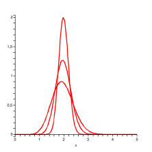
It is clearly seen that is a "fluctuating” version of the deterministic value ; since
| (27) |
we have ; moreover, the variance of is
| (28) |
so that : thus the number of degrees of freedom - imposed by the value of that characterizes and through - rules the fluctuation intensity of around the deterministic value
6 The Extensivity Issue
Still a different and important question was raised in [7], namely the extensivity issue: assuming that a system is composed of two independent subsystems and , the total entropy
is nonextensive (i.e. nonadditive) unless which characterizes the Shannon entropy 333this paragraph concerns only Tsallis entropy since the Harvda-Charvat-Rényi entropy is extensive. A natural question arises then: what kind of dependence should exist between subsystems and so that becomes extensive ?
An answer has been given to this question in the case of Gaussian systems, as follows [17].
Theorem 12
If and then there exists a positive definite matrix and an variate Gaussian vector with covariance matrix such that verifies the extensivity condition
| (29) |
Trying to extend this result to the distributions (3) and (4), one should be careful about the following fact: if is an variate random vector with probability density (3) or (4) and non-extensivity parameter then any single component, say , of is again of the power type, but with a different nonextensivity parameter, say , related to via (23) or equivalently (24):
Thus, the choice of as related to and should be decided. The choice has a long history in the nonextensive literature and already appeared in the paper [18] - for a thorough discussion of the issue and its physical interpretation see [19]. This choice yields the following result.
Theorem 13
and there exists a positive definite matrix and an variate Student-t vector with degrees of freedom and covariance matrix such that
with , and
This result can be extended to the case as follows.
Theorem 14
and , there exists a positive definite matrix and an variate Student-r vector with degrees of freedom and covariance matrix such that
with and
7 Conclusion
In this communication we have presented several results concerning (i) the stability and (ii) the extensivity of power-law random vectors.We have shown that a certain kind of dependence between the components of these vectors, namely the fact that they belong to a larger system that is itself distributed à la power-law, ensures stability of these variables. This property is a direct consequence of the elliptical invariance of the associated or entropy.
In the case of independent components, we have introduced a random-type convolution that ensures stability for the power law distributions.
Finally, we have shown that can be additive if a proper kind of correlation is introduced between the components of the pertinent system, whose properties are to be described by power-law vectors. Further work in progress concerns the extension of this last result to the larger family of elliptically invariant distributions.
References
- [1] Special Issue, Europhysics-news, 36 (2005); Gell-Mann M and Tsallis C Eds. Nonextensive Entropy: Interdisciplinary applications, 2004, Oxford University Press, Oxford.
- [2] Havrda J and Charvát F, Quantification method of classification processes. Concept of structural -entropy 1967 Kybernetika 3 30.
- [3] Vajda I, Axioms for -entropy of a generalized probability scheme ,1968 (Czech) Kybernetika 4 105.
- [4] Daróczy Z, Generalized information functions, 1970 Information and Control 16 36.
- [5] Abe S and Okamoto Y Eds Nonextensive statistical mechanics and its applications 2001(Springer Verlag, Berlin).
- [6] Tsallis C, Possible generalization of Boltzmann-Gibbs statistics, 1988 J. Stat. Phys. 52 479.
- [7] Tsallis C, Nonextensive statistical mechanics, anomalous diffusion and central limit theorems, 2005 Milan Journal of Mathematics 73, 145 (2005)
- [8] Berg C and Vignat C, Linearization coefficients of Bessel polynomials, 2005 [math.PR/0506458]
- [9] Johnson O and Vignat C, Some results concerning maximum Rényi entropy distributions, 2005 [math.PR/0507400]
- [10] Vignat C et al, About closedness by convolution of the Tsallis maximizers, 2004 Physica A, 340 147.
- [11] Beck C and Cohen E G D, Superstatistics, 2003, Physica 322A, 267
- [12] Prato D and Tsallis C, Nonextensive foundation of Lévy distributions, August 1999 Physical Review E 60-2
- [13] Chu K C, Estimation and decision for linear systems with elliptical random processes, 1973 IEEE Trans. On Automatic Control 18499-505
- [14] Vignat C and Plastino A, Poincaré’s Observation and the Origin of Tsallis Generalized Canonical Distributions, [cond-mat/0509689], to appear in Physica A
- [15] F. Barthe et al, A Note on Simultaneous Polar and Cartesian Decomposition, 2003 ,Geometric Aspects of Functional Analysis Springer Lecture Notes in Mathematics 1807 1-19.
- [16] Oliveira F A et al, Scaling transformation of random walk distributions in a lattice June 2000, Physical Review E 61-6 7200-7203
- [17] Vignat C et al, Correlated Gaussian systems exhibiting additive power-law entropies Physics Letters A in Press.
- [18] Curado E M F and Tsallis C, Generalized statistical mechanics: connection with thermodynamics, 1991, J. Phys. A 24 L69.
- [19] Ferri G L et al, Equivalence of the four versions of Tsallis’ statistics, 2005, Journal of Statistical Mechanics P04009.