cond-mat/0602009

Abstract

We review the present status of the superconductivity solution

for an ideal charged boson system, with suggestions for possible

improvement.

———————————-

A dedication in celebration of the 90th birthday of Professor V. L. Ginzburg

*  This research was supported in part by the U. S. Department of Energy Grant

DE-FG02-92ER-40699

1. Introduction

An ideal charged boson system is of interest because of the simplicity in its formulation and yet the complexity of its manifestations. The astonishingly complicated behavior of this idealized system may provide some insight to the still not fully understood properties of high $T_{c}$ superconductivity. As is well known, R. Schafroth[1] first studied the superconductivity of this model fifty years ago. In this classic paper he concluded that at zero temperature $T=0$ and in an external constant magnetic field $H$, there is a critical field

$$(H_{c})_{Sch}=e\rho/2m$$

with $\rho$ denoting the overall number density of the charged bosons and $m$, $e$ their mass and electric charge respectively; the system is in the super phase when $H<H_{c}$, and in the normal phase when $H>H_{c}$. Due to an oversight, Schafroth neglected the exchange part of the electrostatic energy, which invalidates his conclusion as was pointed out in a 1990 paper [2] by Friedberg, Lee and Ren (FLR). This oversight when corrected makes the ideal charged boson model even more interesting. Some aspects of this simple model are still not well understood.

In what follows we first review the Schafroth solution and then the FLR corrections. Our discussions are confined only to $T=0$.

2. Hamiltonian and Schafroth Solution

Let $\phi({\bf r})$ be the charged boson field operator and $\phi^{\dagger}({\bf r})$ its hermitian conjugate, with their equal-time commutator given by

$$[\phi({\bf r}),~{}\phi^{\dagger}({\bf r}^{\prime})]=\delta^{3}({\bf r}-{\bf r}^{\prime}).$$

These bosons are non-relativistic, enclosed in a large cubic volume $\Omega=L^{3}$ and with an external constant background charge density $-e\rho_{ext}~{}$ so that the integral of the total charge density

$$eJ_{0}\equiv e\phi^{\dagger}\phi-e\rho_{ext}$$

is zero. The Coulomb energy operator is given by

$$H_{Coul}=\frac{e^{2}}{8\pi}\int~{}|~{}{\bf r}-{\bf r}^{\prime}|^{-1}~{}:J_{0}({\bf r})J_{0}({\bf r}^{\prime}):~{}d^{3}rd^{3}r^{\prime}$$

where $:~{}:$ denotes the normal product in Wick’s notation[3] so as to exclude the Coulomb self-energy.

Expand the field operator $\phi({\bf r})$ in terms of a complete orthonormal set of $c$-number function $\{f_{i}({\bf r})\}$:

$$\phi({\bf r})=\sum\limits_{i}a_{i}f_{i}({\bf r})$$

with $a_{i}$ and its hermitian conjugate $a_{i}^{\dagger}$ obeying the commutation relation $[a_{i},~{}a_{j}^{\dagger}]=\delta_{ij}$, in accordance with (2.1). Take a normalized state vector $|>$ which is also an eigenstate of all $a_{i}^{\dagger}a_{i}$ with

$$a_{i}^{\dagger}a_{i}|>=n_{i}|>.$$

For such a state, the expectation value of the Coulomb energy $E_{Coul}$ can be written as a sum of three terms:

$$<|H_{Coul}|>=E_{ex}+E_{dir}+E_{dir}^{\prime}$$

where

$$E_{ex}=\sum\limits_{i\neq j}\frac{e^{2}}{8\pi}\int d^{3}rd^{3}r^{\prime}|~{}{\bf r}-{\bf r}^{\prime}|^{-1}n_{i}n_{j}f_{i}^{*}({\bf r})f_{j}^{*}({\bf r}^{\prime})f_{i}({\bf r}^{\prime})f_{j}({\bf r})$$

$$E_{dir}=\frac{e^{2}}{8\pi}\int d^{3}rd^{3}r^{\prime}|~{}{\bf r}-{\bf r}^{\prime}|^{-1}<|J_{0}({\bf r})|><|J_{0}({\bf r}^{\prime})|>$$

and

$$E_{dir}^{\prime}=-\sum\limits_{i}\frac{e^{2}}{8\pi}\int d^{3}rd^{3}r^{\prime}|~{}{\bf r}-{\bf r}^{\prime}|^{-1}n_{i}|f_{i}({\bf r})|^{2}|f_{i}({\bf r}^{\prime})|^{2}.$$

The last term $E_{dir}^{\prime}$ is the subtraction, recognizing that in Wick’s normal product each particle does not interact with itself.

In the Schafroth solution, for the super phase at $T=0$ all particles are in the zero momentum state; therefore, on account of (2.2) the ensemble average of $J_{0}$ is zero and so is the Coulomb energy. For the normal phase, take the magnetic field ${\bf B}=B\hat{z}$ with $B$ uniform and pick its gauge field ${\bf A}=Bx\hat{y}$. At $T=0$, let

$$f_{i}({\bf r})=e^{ip_{i}y}\psi_{i}(x).$$

Schafroth assumed $p_{i}=eBx_{i}$ with $x_{i}$ spaced at regular intervals $\lambda=2\pi/eBL$, which approaches zero as $L\rightarrow\infty$. This makes the boson density uniform and therefore $E_{dir}=0$. In the same infinite volume limit, one can show readily that $\Omega^{-1}E_{dir}^{\prime}\rightarrow 0$. Since Schafroth omitted $E_{ex}$, his energy consists only of

$$E_{field}=\int d^{3}r\frac{1}{2}~{}B^{2},$$

$$E_{mech}=\sum\limits_{i}n_{i}\int d^{3}r\frac{1}{2m}~{}\bigg{(}\frac{d\psi_{i}}{dx}\bigg{)}^{2}$$

and

$$E_{dia}=\sum\limits_{i}n_{i}\int d^{3}r\frac{1}{2m}~{}(p_{i}-eA_{y}(x))^{2}$$

$$~{}~{}~{}~{}~{}~{}~{}~{}=\sum\limits_{i}n_{i}\int d^{3}r\frac{eB}{2m}~{}(x-x_{i})^{2}.$$

The sum of (2.10) and (2.11) gives the usual cyclotron energy

$$E_{mech}+E_{dia}=\sum\limits_{i}n_{i}~{}\frac{eB}{2m}.$$

Combining with (2.9), Schafroth derived the total Helmholtz free energy density in the normal phase at zero temperature to be

$$F_{n}=\frac{1}{2}~{}B^{2}+\frac{e\rho}{2m}~{}B$$

(Throughout the paper, we take $e$ and $B$ to be positive, since all energies are even in these parameters.)

The derivation of (2.13) is, however, flawed by the omission of $E_{ex}$. It turns out that for the above particle wave function (2.8), when $x_{i}-x_{j}$ is $<<$ the cyclotron radius $a=(eB)^{-\frac{1}{2}}$, the coefficient of $n_{i}n_{j}$ in $E_{ex}$ is proportional to $|x_{i}-x_{j}|^{-1}$. Hence $\Omega^{-1}E_{ex}$ becomes $\infty$ logarithmically as the spacing $\lambda\rightarrow 0$.

3. Corrected Normal State at High Density

In this and the next section, we review the FLR analysis for the high density case, when $\rho>r_{b}^{-3}$ where $r_{b}=$ Bohr radius $=4\pi/me^{2}$.

a. Strong field. We discuss first the case when $B$ is $>>(m\rho)^{\frac{1}{2}}$, so that the Coulomb correction to the magnetic energy (2.13) can be treated as a perturbation. To find the groundstate energy, we shall continue to assume (2.8) with $p_{i}=eBx_{i}$ and $x_{i}$ equally spaced at interval $\lambda$, but keeping $\lambda\neq 0$. Now as $\Omega\rightarrow\infty$, $\Omega^{-1}E_{dir}^{\prime}$ remains zero, but $\Omega^{-1}E_{dir}$ in fact increases as $\lambda^{2}$ for $\lambda>>a$, the cyclotron radius. The lowest value of $E_{dir}+E_{ex}$ are both complicated in this range. The minimization can be done exactly, yielding

$$\lambda=\pi a\lambda_{0}$$

where

$$1-\bigg{(}\frac{\pi}{2}\bigg{)}^{\frac{1}{2}}\lambda_{0}=\lambda_{0}^{2}\sum\limits_{\mu=1}^{\infty}e^{-2\mu^{2}/\lambda_{0}}$$

The sum of $E_{dir}$ and $E_{ex}$ is found to be proportional to $1/B$. Hence, (2.13) is replaced by

$$F_{n}=\frac{1}{2}~{}B^{2}+\frac{e\rho}{2m}~{}B+\frac{e\rho^{2}}{B}~{}\gamma_{n}$$

with

$$\gamma_{n}=\gamma_{dir}+\gamma_{ex}=0.00567+0.00715=0.0128.$$

b. Weak field. Clearly (3.3) cannot be extended to $B\rightarrow 0$, as the last term would diverge. In its derivation the $\psi_{i}(x)$ in (2.8) is taken to be the usual simple harmonic oscillator wave function determined by the magnetic field $B$ only, without regard to $E_{Coul}$. This is valid only when $B>>(m\rho)^{\frac{1}{2}}$. For much smaller $B$, we may consider a configuration in which the function $\psi_{i}(x)$ is spread out flat over a width $\lambda-l$, then drops to zero sinusoidally over a smaller width $l$ on each side. Neighboring $\psi_{i}$ overlap only in the strips of width $l$.Thus, it can be arranged that $\sum\limits_{i}|\psi_{i}(x)|^{2}$ is uniform and hence

$$E_{dir}=0.$$

For sufficiently weak $B$, we find $\lambda>>$ the London length $\lambda_{L}=(e^{2}\rho/m)^{-\frac{1}{2}}$. We must then drop the assumption that $B$ is uniform; it is largest in the overlap region and drops to zero over the length $\lambda_{L}$ in either side. Let $\overline{B}$ be the average of $B$ over $\Omega$ and $\overline{a}\equiv(e\overline{B})^{-\frac{1}{2}}$ the corresponding ”cyclotron radius”. It is then found that

$$\lambda=\frac{\pi\overline{a}^{2}}{\epsilon\lambda_{L}},$$

$$l=\lambda_{L}\epsilon^{2}<<\lambda_{L}$$

where

$$\epsilon=\bigg{(}\frac{\pi^{5}}{8m^{2}\lambda_{L}^{2}}\bigg{)}^{1/7}<<1$$

is independent of $\overline{B}$. The energies $E_{mech}$, $E_{ex}$, $E_{dia}$ are all proportional to $\overline{B}$, and one obtains for the free energy density

$$F_{n}=\frac{1}{2}~{}\overline{B}^{2}+\frac{e\rho}{m}~{}\eta\overline{B}$$

with

$$\eta=\frac{7\pi}{16\epsilon}>>1,$$

much bigger than the Schafroth result.

c.Intermediate field. Let

$$B_{1}=e\rho/m,~{}~{}~{}B_{2}=(m\rho)^{\frac{1}{2}}$$

Between the above strong field case $B>>B_{2}$ and the weak field case when $\overline{B}<<\eta B_{1}$, we have the regime when $\psi$ remains flat as in the previous section, but with $\lambda_{L}>>\lambda\geq l$. Hence, $E_{dir}=0$ as in (b), but $B$ is uniform as in (a). One obtains an estimate

$$F_{n}=\frac{1}{2}~{}B^{2}+\frac{5}{32}~{}B_{0}^{7/5}B^{3/5}$$

where

$$B_{0}=\bigg{(}\frac{16}{3}\pi m\lambda_{L}\bigg{)}^{2/7}B_{1}.$$

The formulas (3.3-4), (3.9-10) and (3.12-13) are strictly upper bounds, which might be improved with better wave functions. We hope these to be good estimates.

a. $H_{c_{1}}$. The coherent length $\xi$ governing the disappearance of the normal phase outside a vortex is found from the Ginzburg-Landau (G.-L.) equation[4] to be

$$\xi=(2\lambda_{L}/m)^{\frac{1}{2}}.$$

and hence (taking $m\lambda_{L}>>1$) $\lambda_{L}>>\xi$ so that we should have a type II superconductor, with the critical field for vortex penetration

$$H_{c_{1}}\cong\frac{1}{2}B_{1}[~{}\ln(\lambda_{L}/\xi)+1.623~{}]$$

in which the constant differs from that given by the G.-L. equation because of the long range Coulomb field.

However, in Schafroth’s solution because of (2.13), his normal phase would begin to exist at

$$(H_{c})_{Sch}=\frac{1}{2}~{}B_{1}<<H_{c_{1}},$$

above which $(F_{n}-BH)_{Sch}$ would also be lower than that for the super phase, making it a Type I superconductor. But Schafroth’s solution is invalid; (2.13) must be replaced by (3.9) at low $B$, giving

$$H_{c}=\eta B_{1}$$

with $\eta>>\frac{1}{2}$, as shown in (3.10).

Next, we compare the above corrected $H_{c}$ with $H_{c_{1}}$. Using (4.1), we write (4.2) as

$$H_{c_{1}}=\bigg{(}\frac{7}{8}~{}\ln\zeta\bigg{)}B_{1}$$

where

$$\ln\zeta=\frac{4}{7}~{}\bigg{(}\frac{1}{2}\ln\frac{m\lambda_{L}}{2}+1.623\bigg{)}.$$

Likewise, because of (3.8) and (3.10), the parameter $\eta$ in (4.4) can also be expressed in terms of the same $\zeta$:

$$\eta=\kappa~{}\zeta$$

with the constant $\kappa$ given by

$$\kappa=\frac{7}{8}~{}\bigg{(}\frac{\pi}{2}~{}e^{-3.246}\bigg{)}^{2/7}.$$

Thus,

$$\frac{H_{c}}{H_{c_{1}}}=\frac{8\kappa}{7}~{}\frac{\zeta}{\ln\zeta}.$$

Now $\zeta/\ln\zeta$ has a minimum$=e$ when $\zeta=e$. Thus,

$$\frac{H_{c}}{H_{c_{1}}}>\bigg{(}\frac{\pi}{2}\bigg{)}^{2/7}e^{0.07}>1,$$

and the system is indeed a Type II superconductor.

b. Vortices. Once $H=H_{c_{1}}+$, the vortices appear and soon become so numerous that their typical separation is of the order of $\lambda_{L}$. This gives an average $B$ of the order of $B_{1}=e\rho/m$.

c. $B>B_{1}$. To increase $B$ further, it is necessary to increase $H$ on account of the interaction energy between vortices. The vortex separation distance is of the order of the cyclotron radius $a=(eB)^{-\frac{1}{2}}$. In the regime $\xi<<a<<\lambda_{L}$ (correspondingly, $B_{2}>>B>>B_{1}$), the vortices naturally form a lattice to minimize their interaction energy. An involved calculation gives the Helmholtz free energy density at $T=0$ to be

$$F_{s}=\frac{1}{2}B^{2}+\frac{1}{4}B_{1}B(\ln\frac{B_{2}}{B}+{\sf const})$$

where $B_{2}=(m\rho)^{\frac{1}{2}}$ and the constant is

$$~{}~{}~{}~{}~{}~{}~{}~{}~{}~{}-\ln 4\pi+\left\{\begin{array}[]{ll}4.068~{},~{}~{}~{}{\sf square~{}~{}lattice}\\ 4.048~{},~{}~{}~{}{\sf triangular~{}~{}lattice}.\end{array}\right.~{}~{}~{}~{}~{}~{}~{}~{}~{}~{}~{}~{}~{}~{}~{}~{}~{}~{}~{}~{}~{}~{}~{}~{}~{}~{}(4.12)$$

d. $B>>B_{2}$. In this case of very strong magnetic field when the cyclotron radius and the separation distance are both much less than $\xi$ (but we assume that the system remains non-relativistic). The free energy density is dominated by the RHS of (2.13). However, there is still a super phase whose wave function is assumed to be given by the Abrikosov solution, giving by Eq.(8) of Ref.[5] and its Coulomb energy is calculated as a perturbation. The result for the Helmholtz energy density in the super phase is

$$F_{s}=\frac{1}{2}B^{2}+\frac{e\rho}{2m}B+\frac{e\rho^{2}}{B}\gamma_{s}$$

with

$$~{}~{}~{}~{}~{}~{}~{}~{}~{}~{}~{}~{}\gamma_{s}=\left\{\begin{array}[]{ll}0.01405~{},~{}~{}~{}{\sf square~{}~{}lattice}\\ 0.01099~{},~{}~{}~{}{\sf triangular~{}~{}lattice}.\end{array}\right.~{}~{}~{}~{}~{}~{}~{}~{}~{}~{}~{}~{}~{}~{}~{}~{}~{}~{}~{}~{}~{}~{}~{}~{}~{}~{}~{}~{}(4.14)$$

e. $H_{c_{2}}$. The super phase regimes of Sections 4a-b, 4c, 4d correspond (with respect to the value of $B$ or its average $\overline{B}$) to those of the normal phase regimes discussed in 3b, 3c and 3a respectively. Since, for the triangular lattice, a comparison of (4.14) with (3.4) gives $\gamma_{s}=0.01099<\gamma_{n}=0.0128$, we see that $F_{s}<F_{n}$ for the same $B>>B_{2}$. Similarly, $F_{s}<F_{n}$ for the same $B$ in the regimes $B_{2}>>B>>B_{1}$ and $B<<B_{1}$. From these results and that $H=dF/dB$ is monotonic in $B$, one can readily deduce that the Legendre transform

$$\tilde{F}=F-BH$$

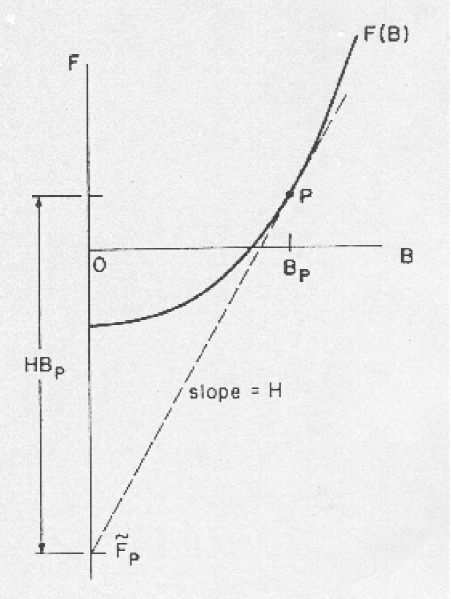
Figure 1: Graphical construction of $\tilde{F}=F-HB$. At any point $P$ on the curve $F(B)$, the intercept of its tangent with ordinate gives $\tilde{F}$, since the tangent has a slope $H$. The subscript $P$ denotes the values of $B$ and $\tilde{F}$ at $P$.

satisfies $\tilde{F}_{s}<\tilde{F}_{n}$ for the same $H$ in all these regions. (See Figure 1)

From this it seems possible that

$$H_{c_{2}}=\infty;$$

the super phase may persist at high density for all values of the magnetic field.

f. Remarks. In the problem discussed in Ref.[5], the Ginzburg-Landau function $\Psi$ is an order parameter, whereas our $f_{i}(r)$ are single particle wave functions. Nevertheless, except for the constant in (4.2), the two problems have the same physics content at high $\rho$ when $H<<B_{2}$. For higher field when $H\geq B_{2}$, the Ginzburg-Landau $\Psi$ should vanish; however, this is not true in our problem. At $T=0$, we place all the particles in the coherent state, making the charge density to vary greatly within a unit lattice cell. Our result (4.14) favoring a triangular lattice is unrelated to that of [5], because the ratio parameter $<|\Psi|^{4}>/<|\Psi|^{2}>^{2}$ in [5] does not appear in our problem. The lattice dependence in our problem is electrostatic in origin.

5. Low Density at Zero Field

a. Normal Phase. At very low density and with zero magnetic field, $E_{dir}^{\prime}$ of (2.7) becomes important. The lowest energy is now achieved by placing the individual charges in separate cells forming a lattice, with little or no overlap. Hence $E_{ex}$ can be disregarded, and a trial wave function leads in the limit $\rho\rightarrow 0$ to

$$N^{-1}(E_{Coul}+E_{mech})=-\alpha_{n}\frac{e^{2}}{4\pi R}$$

where

$$(4\pi/3)R^{3}=\rho^{-1}~{}~{}~{}{\sf and}~{}~{}~{}\alpha_{n}\cong 0.9$$

very closely. The above formula (5.1) is valid for $\rho<<r_{b}^{-3}$, with $r_{b}$ the Bohr radius.

b. Super Phase. In the same limit, the super phase energy also becomes negative, as shown by a Bogolubov-type transformation[6-8]. This leads to

$$N^{-1}(E_{Coul}+E_{mech})=-\alpha_{s}\frac{e^{2}}{4\pi R}$$

with

$$0.316<\alpha_{s}<0.558.$$

Thus, $\alpha_{s}<\alpha_{n}$ and the normal phase holds at $\rho<<r^{-3}_{b}$.

c. Critical Density. As $\rho$ increases, (5.1-2) serves only as a lower bound; i.e.,

$$N^{-1}(E_{Coul}+E_{mech})>-(0.9)\frac{e^{2}}{4\pi R}.$$

For the normal phase, when $\rho$ approaches $r^{-3}_{b}$, the single particle wave function leading to (5.1-2) can no longer fit without overlap. We confine each particle within a cube, give it a $r^{-1}\sin qr$ wave function as a trial function, just avoiding overlap so that $E_{ex}=0$. With approximation neglecting the distinction between sphere and cube, we find

$$N^{-1}E_{mech}=\frac{\pi^{2}}{2mR^{2}},~{}~{}~{}N^{-1}E_{Coul}=-\frac{e^{2}}{4\pi R}K_{n}$$

where

$$K_{n}\approx 0.76~{}.$$

Equating the above $N^{-1}(E_{Coul}+E_{mech})$ for the normal phase with the corresponding expression (5.3) for the super phase, we find the critical density $\rho_{c}$ given by

$$r_{b}^{3}~{}\rho_{c}=\frac{6}{\pi^{7}}~{}(K_{n}-\alpha_{s})^{3}.$$

The system is in the normal state when $\rho<\rho_{c}$, and in the super state when $\rho>\rho_{c}$. (Eq.(4.12) in the FLR paper is equivalent to (5.8), but without the subtraction of $K_{n}$ by $\alpha_{s}$.)

6. Further Improvement

Although the FLR paper (66 pages in the Annals of Phys.) is quite lengthy, several important questions remain open.

a. The energies in above sections 3 and 4 are all upper bounds obtained from trial functions. Perhaps a better trial function, like changing slabs into cylinders, might lower these bounds and put into questions some of the FLR conclusions. Also a numerical calculation exploring the transition regions would be valuable in case there are surprises, particularly when $B\sim B_{2}$. In this connection we note that, e.g., in (4.9) the relevant factor in $\zeta/\ln\zeta$ is $(m\lambda_{L})^{2/7}/\ln(m\lambda_{L})$, which becomes large when $m\lambda_{L}\rightarrow\infty$; yet, it is $<1$ when $m\lambda_{L}=100$ and only near but still less than $2$ when $m\lambda_{L}$ is $2000$.

b. The calculation of the above (5.6-7), i.e., Section 4.2 in the FLR paper, can be improved in several ways. First, consider the integral $\frac{1}{2}\int J_{0}Vd^{3}r$, with $V$ the potential due to $J_{0}$. Because the spatial integral of $J_{0}$ is zero, and since each particle does not interact with itself we have

$$N^{-1}(E_{dir}+E_{dir}^{\prime})=e\int\psi^{2}_{0}({\bf r})\overline{V}({\bf r})d^{3}r$$

where $\psi_{0}({\bf r})$ is located inside a sphere, centered at zero, and $\overline{V}({\bf r})$ is due to all of $J_{0}$ except the term due to $\psi^{2}_{0}$. Second, there is no need to ignore the distinction between sphere and cube. Using theorems from electrostatics, one can reduce (6.1) to the solution of a Madelung problem with like charges at lattice points and a background charge filling all space, plus a correction $\frac{1}{6}e^{2}\rho\int\psi^{2}_{0}({\bf r})r^{2}d^{3}r$. This correction can be combined with $E_{mech}$ to optimize $\psi_{0}$, and the Madelung problem can be done by known methods. Third, the energy can probably be reduced by placing the centers of the particle wave functions on a body-centered cubic lattice, as the cell available to each particle would then be more nearly spherical than a cube.

c. Both FLR and the present paper have left open the question of what happens at low density and high field. It would be surprising if the boundary between super and normal phases were independent of the magnetic field strength. In the $H$ versus $\rho$ phase diagram at $T=0$ and high $H$, does the boundary between normal and super phases bend towards lower $\rho$, or towards higher?

7. Comment

The two most striking results in our paper are $H_{c_{1}}<H_{c}$, making the superconductor Type II instead of Type I, and that $H_{c_{2}}$ might be infinite. An improvement in the weak field normal trial function (the above Section 3b) might invalidate the first conclusion by lowering $\eta$ in (3.9). An improvement in the strong field normal trial function (Section 3a) could invalidate the second conclusion by lowering $\gamma_{n}$ in (3.3).

The field of condensed matter physics has received from its very beginning many deep and beautiful contributions from Russian physicists and masters L. D. Landau, V. L. Ginzburg, N. N. Bogolubov, A. A. Abrikosov, A. M. Polyakov and others. It is our privilege to add this small piece to honor this great and strong tradition and to celebrate the 90th birthday of V. L. Ginzburg.

References

[1] M. R. Schafroth, Phys. Rev. 100(1955),463.
[2] R. Friedberg, T. D. Lee and H. C. Ren, Ann. Phys. 208(1991),149.
[3] G. C. Wick, Phys. Rev. 80(1950),268.
[4] V. L. Ginzburg and L. D. Landau, J. Expt. Theort. Phys.(USSR)
20(1950),1064.
[5] A. A. Abrikosov, Soviet Phys. JETP 5(1957),1174.