Quantum phase transitions
from topology in momentum space

Quantum phase transitions from topology in momentum space

Many quantum condensed matter systems are strongly correlated and strongly interacting fermionic systems, which cannot be treated perturbatively. However, physics which emerges in the low-energy corner does not depend on the complicated details of the system and is relatively simple. It is determined by the nodes in the fermionic spectrum, which are protected by topology in momentum space (in some cases, in combination with the vacuum symmetry). Close to the nodes the behavior of the system becomes universal; and the universality classes are determined by the toplogical invariants in momentum space. When one changes the parameters of the system, the transitions are expected to occur between the vacua with the same symmetry but which belong to different universality classes. Different types of quantum phase transitions governed by topology in momentum space are discussed in this Chapter. They involve Fermi surfaces, Fermi points, Fermi lines, and also the topological transitions between the fully gapped states. The consideration based on the momentum space topology of the Green’s function is general and is applicable to the vacua of relativistic quantum fields. This is illustrated by the possible quantum phase transition governed by topology of nodes in the spectrum of elementary particles of Standard Model.

1 Introduction.

There are two schemes for the classification of states in condensed matter physics and relativistic quantum fields: classification by symmetry (GUT scheme) and by momentum space topology (anti-GUT scheme).

For the first classification method, a given state of the system is characterized by a symmetry group $H$ which is a subgroup of the symmetry group $G$ of the relevant physical laws. The thermodynamic phase transition between equilibrium states is usually marked by a change of the symmetry group $H$. This classification reflects the phenomenon of spontaneously broken symmetry. In relativistic quantum fields the chain of successive phase transitions, in which the large symmetry group existing at high energy is reduced at low energy, is in the basis of the Grand Unification models (GUT) UnificationModel ; Unification . In condensed matter the spontaneous symmetry breaking is a typical phenomenon, and the thermodynamic states are also classified in terms of the subgroup $H$ of the relevant group $G$ (see e.g, the classification of superfluid and superconducting states in Refs. VolovikGorkov1985 ; VollhardtWoelfle ). The groups $G$ and $H$ are also responsible for topological defects, which are determined by the nontrivial elements of the homotopy groups $\pi_{n}(G/H)$; cf. Ref. TopologyReview1 .

The second classification method reflects the opposite tendency – the anti Grand Unification (anti-GUT) – when instead of the symmetry breaking the symmetry gradually emerges at low energy. This method deals with the ground states of the system at zero temperature ($T=0$), i.e., it is the classification of quantum vacua. The universality classes of quantum vacua are determined by momentum-space topology, which is also responsible for the type of the effective theory, emergent physical laws and symmetries at low energy. Contrary to the GUT scheme, where the symmetry of the vacuum state is primary giving rise to topology, in the anti-GUT scheme the topology in the momentum space is primary while the vacuum symmetry is the emergent phenomenon in the low energy corner.

At the moment, we live in the ultra-cold Universe. All the characteristic temperatures in our Universe are extremely small compared to the Planck energy scale $E_{\rm P}$. That is why all the massive fermions, whose natural mass must be of order $E_{\rm P}$, are frozen out due to extremely small factor $\exp(-E_{\rm P}/T)$. There is no matter in our Universe unless there are massless fermions, whose masslessness is protected with extremely high accuracy. It is the topology in the momentum space, which provides such protection.

For systems living in 3D space, there are four basic universality classes of fermionic vacua provided by topology in momentum space VolovikBook ; Horava :

(i) Vacua with fully-gapped fermionic excitations, such as semiconductors and conventional superconductors.

(ii) Vacua with fermionic excitations characterized by Fermi points – points in 3D momentum space at which the energy of fermionic quasiparticle vanishes. Examples are provided by superfluid ³He-A and also by the quantum vacuum of Standard Model above the electroweak transition, where all elementary particles are Weyl fermions with Fermi points in the spectrum. This universality class manifests the phenomenon of emergent relativistic quantum fields at low energy: close to the Fermi points the fermionic quasiparticles behave as massless Weyl fermions, while the collective modes of the vacuum interact with these fermions as gauge and gravitational fields.

(iii) Vacua with fermionic excitations characterized by lines in 3D momentum space or points in 2D momentum space. We call them Fermi lines, though in general it is better to characterize zeroes by co-dimension, which is the dimension of ${\bf p}$-space minus the dimension of the manifold of zeros. Lines in 3D momentum space and points in 2D momentum space have co-dimension 2: since $3-1=2-0=2$; compare this with zeroes of class (ii) which have co-dimension $3-0=3$. The Fermi lines are topologically stable only if some special symmetry is obeyed. Example is provided by the vacuum of the high $T_{c}$ superconductors where the Cooper pairing into a $d$-wave state occurs. The nodal lines (or actually the point nodes in these effectively 2D systems) are stabilized by the combined effect of momentum-space topology and time reversal symmetry.

(iv) Vacua with fermionic excitations characterized by Fermi surfaces. The representatives of this universality class are normal metals and normal liquid ³He. This universality class also manifests the phenomenon of emergent physics, though non-relativistic: at low temperature all the metals behave in a similar way, and this behavior is determined by the Landau theory of Fermi liquid – the effective theory based on the existence of Fermi surface. Fermi surface has co-dimension 1: in 3D system it is the surface (co-dimension $=3-2=1$), in 2D system it is the line (co-dimension $=2-1=1$), and in 1D system it is the point (co-dimension $=1-0=1$; in one dimensional system the Landau Fermi-liquid theory does not work, but the Fermi surface survives).

The possibility of the Fermi band class (v), where the energy vanishes in the finite region of the 3D momentum space and thus zeroes have co-dimension 0, has been also discussed Khodel1990 ; NewClass ; Shaginyan ; Khodel2005 . It is believed that this the so-called Fermi condensate may occur in strongly interacting electron systems PuCoGA₅ and CeCoIn₅ Khodel2005b . Topologically stable flat band may exist in the spectrum of fermion zero modes, i.e. for fermions localized in the core of the topological objects Volovik1994 .

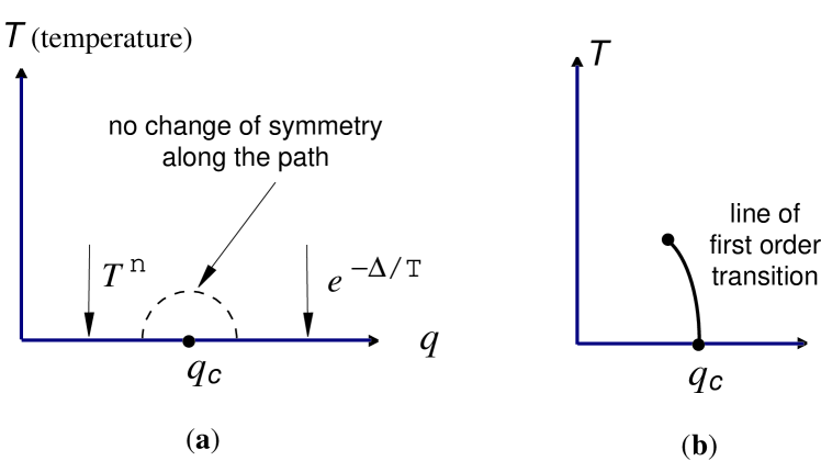
Figure 1: Quantum phase transition between two ground states with the same symmetry but of different universality class – gapless at $q<q_{c}$ and fully gapped at $q>q_{c}$ – as isolated point (a) as the termination point of first order transition (b)

The phase transitions which follow from this classification scheme are quantum phase transitions which occur at $T=0$ Sachdev . It may happen that by changing some parameter $q$ of the system we transfer the vacuum state from one universality class to another, or to the vacuum of the same universality class but different topological quantum number, without changing its symmetry group $H$. The point $q_{c}$, where this zero-temperature transition occurs, marks the quantum phase transition. For $T\neq 0$, the second order phase transition is absent, as the two states belong to the same symmetry class $H$, but the first order phase transition is not excluded. Hence, there is an isolated singular point $(q_{c},0)$ in the $(q,T)$ plane (Fig. 1(a)), or the end point of the first order transition (Fig. 1(b)).

The quantum phase transitions which occur in classes (iv) and (i) or between these classes are well known. In the class (iv) the corresponding quantum phase transition is known as Lifshitz transition Lifshitz , at which the Fermi surface changes its topology or emerges from the fully gapped state of class (i), see Sec. 2.2. The transition between the fully gapped states characterized by different topological charges occurs in 2D systems exhibiting the quantum Hall and spin-Hall effect: this is the plateau-plateau transition between the states with different values of the Hall (or spin-Hall) conductance (see Sec. 5). The less known transitions involve nodes of co-dimension 3 Book1 ; QPT ; SplittingPreprint ; Gurarie ; BotelhoPWavw (Sec. 3 on Fermi points) and nodes of co-dimension 2 Botelho ; Borkowski ; Duncan ; WenZee ( Sec. 4 on nodal lines). The quantum phase transitions involving the flat bands of class (v) are discussed in Ref. Volovik1994 .

2 Fermi surface and Lifshitz transition

2.1 Fermi surface as a vortex in ${\bf p}$-space

In ideal Fermi gases, the Fermi surface at $p=p_{F}=\sqrt{2\mu m}$ is the boundary in ${\bf p}$-space between the occupied states ($n_{\bf p}=1$) at $p^{2}/2m<\mu$ and empty states ($n_{\bf p}=0$) at $p^{2}/2m>\mu$. At this boundary (the surface in 3D momentum space) the energy is zero. What happens when the interaction between particles is introduced? Due to interaction the distribution function $n_{\bf p}$ of particles in the ground state is no longer exactly 1 or 0. However, it appears that the Fermi surface survives as the singularity in $n_{\bf p}$. Such stability of the Fermi surface comes from a topological property of the one-particle Green’s function at imaginary frequency:

$$G^{-1}=i\omega-\frac{p^{2}}{2m}+\mu~{}.$$ (1)

Let us for simplicity skip one spatial dimension $p_{z}$ so that the Fermi surface becomes the line in 2D momentum space $(p_{x},p_{y})$; this does not change the co-dimension of zeroes which remains $1=3-2=2-1$. The Green’s function has singularities lying on a closed line $\omega=0$, $p_{x}^{2}+p_{y}^{2}=p_{F}^{2}$ in the 3D momentum-frequency space $(\omega,p_{x},p_{y})$ (Fig. 2(a)). This is the line of the quantized vortex in the momemtum space, since the phase $\Phi$ of the Green’s function $G=|G|e^{i\Phi}$ changes by $2\pi N_{1}$ around the path embracing any element of this vortex line. In the considered case the phase winding number is $N_{1}=1$. If we add the third momentum dimension $p_{z}$ the vortex line becomes the surface in the 4D momentum-frequency space $(\omega,p_{x},p_{y},p_{z})$ – the Fermi surface – but again the phase changes by $2\pi$ along any closed loop empracing the element of the 2D surface in the 4D momentum-frequency space.

The winding number cannot change by continuous deformation of the Green’s function: the momentum-space vortex is robust toward any perturbation. Thus the singularity of the Green’s function on the Fermi surface is preserved, even when interaction between fermions is introduced. The invariant is the same for any space dimension, since the co-dimension remains 1.

The Green function is generally a matrix with spin indices. In addition, it may have the band indices (in the case of electrons in the periodic potential of crystals). In such a case the phase of the Green’s function becomes meaningless; however, the topological property of the Green’s function remains robust. The general analysis Horava demonstrates that topologically stable Fermi surfaces are described by the group $Z$ of integers. The winding number $N_{1}$ is expressed analytically in terms of the Green’s function VolovikBook :

$$N_{1}={\bf tr}~{}\oint_{C}{dl\over 2\pi i}G(\mu,{\bf p})\partial_{l}G^{-1}(\mu,{\bf p})~{}.$$ (2)

Here the integral is taken over an arbitrary contour $C$ around the momentum-space vortex, and ${\bf tr}$ is the trace over the spin, band and/or other indices.

2.2 Lifshitz transitions

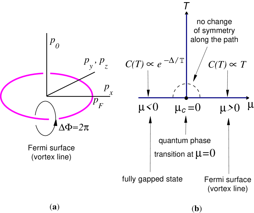
Figure 2: (a) Fermi surface is a topological object in momentum space – a vortex loop. (b) When the chemical potential $\mu$ decreases the loop shrinks and disappears at $\mu<0$. The point $\mu=T=0$ marks the Lifshitz transition between the gapless ground state at $\mu>0$ to the fully gapped vacuum at $\mu<0$

There are two scenarios of how to destroy the vortex loop in momentum space: perturbative and non-perturbative. The non-perturbative mechanism of destruction of the Fermi surface occurs for example at the superconducting transition, at which the spectrum changes drastically and the gap appears. We shall consider this later in Sec. 2.3, and now let us concentrate on the perturbative processes.

Contraction and expansion of vortex loop in ${\bf p}$-space

The Fermi surface cannot be destroyed by small perturbations, since it is protected by topology and thus is robust to perturbations. But the Fermi surface can be removed by large perturbations in the processes which reproduces the processes occurring for the real-space counterpart of the Fermi surface – the loop of quantized vortex in superfluids and superconductors. The vortex ring can continuously shrink to a point and then disappear, or continuously expand and leave the momentum space. The first scenario occurs when one continuously changes the chemical potential from the positive to the negative value: at $\mu<0$ there is no vortex loop in momentum space and the ground state (vacuum) is fully gapped. The point $\mu=0$ marks the quantum phase transition – the Lifshitz transition – at which the topology of the energy spectrum changes (Fig. 2(b)). At this transition the symmetry of the ground state does not changes. The second scenario of the quantum phase transition to the fully gapped states occurs when the inverse mass $1/m$ in Eq.(1) crosses zero.

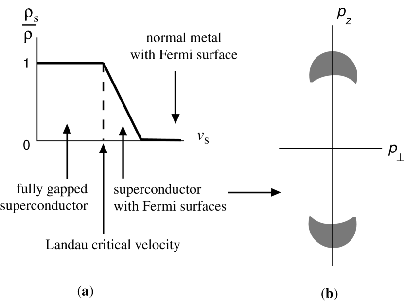
Figure 3: Illustration of Lifshitz transition in superfluid/superconductor at Landau critical velocity. (a) In the presence of the superfluid motion with velocity ${\bf v}_{s}$, the spectrum of quasiparticles is Doppler shifted. In the fully gapped superconductor in Eq.(5) the spectrum becomes $E({\bf p})=\pm\sqrt{(p^{2}/2m-\mu)^{2}+|\Delta|^{2}}+{\bf p}\cdot{\bf v}_{s}$. When the flow velocity exceeds the Landau critical velocity, $v_{L}\approx\Delta/p_{F}$ if $\Delta\ll\mu$, the positive branch crosses zero energy level. Typically this leads to instability, but in some cases, for example, in superfluid ³He-B, the superfluidity is not destroyed. In this case the Landau critical velocity marks the quantum phase transition at which two Fermi surfaces with $E({\bf p})=0$ emerge in the superfluid state (b). Liquid remains superfluid, but the density of the fermionic states is nonzero due to Fermi surfaces. Due to that the normal component of the liquid becomes nonzero even at $T=0$, as a result the density of the superfluid component $\rho_{s}$ (the prefactor in the superfluid current ${\bf j}_{s}=\rho_{s}{\bf v}_{s}$) is reduced compared with its value $\rho$ below the threshold. See also Sec. 26.1 in Ref. VolovikBook .

Similar Lifshitz transitions from the fully gapped state to the state with the Fermi surface may occur in superfluids and superconductors. This happens, for example, when the superfluid velocity crosses the Landau critical velocity [Fig. 3]. The symmetry of the order parameter does not change across such a quantum phase transition. On the other examples of the Fermi surface in superfluid/superconducting states in condensed matter and quark matter see Gubankova ). In the non-superconduting states, the transition from the gapless to gapped state is the metal-insulator transition. The Mott transition also belongs to this class.

Reconnection of vortex lines in ${\bf p}$-space

The Lifshitz transitions involving the vortex lines in ${\bf p}$-space may occur between the gapless states. They are accompanied by the change of the topology of the Fermi surface itself. The simplest example of such a phase transition discussed in terms of the vortex lines is provided by the reconnection of the vortex lines. In Fig. 4 the two-dimensional system is considered with the saddle point spectrum $E({\bf p})=p_{x}^{2}-p_{y}^{2}-\mu$. The reconnection quantum transition occurs at $\mu=0$. The three-dimensional systems, in which the Fermi surface is a 2D vortex sheet in the 4D space $(\omega,p_{x},p_{y},p_{z})$, may experience the more complicated topological transitions.

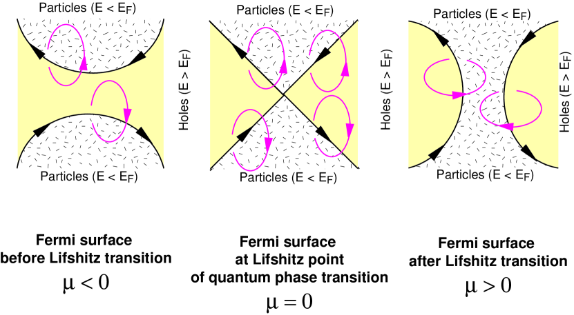
Figure 4: Lifshitz transition with change of the Fermi surface topology as reconnection of vortex lines in momentum space. The direction of the ”circulation” around the vortex lines (grey arrows) and ”vorticity” along the vortex lines (black arrows) are shown

2.3 Metal-superconductor transition

The transition to superconducting state, even if it occurs at $T=0$, does not belong to the class of the quantum phase transitions which we discuss in this review, because it is the consequence of the spontaneously broken symmetry and does not occur perturbatively. Let us discuss this transition from the point of view of the momentum-space topology.

Topology of Gor’kov function across the superconducting transition

Let us first note that the breaking of $U(1)$ symmetry is not the sufficient condition for superfluidity or superconductivity. For example, the $U(1)$ symmetry of the atoms A which is the result of conservation of the number $N_{A}$ of A atoms, may be violated simply due to possibility of decay of atom A to atom B. But this does not lead to superfluidity, and the Fermi surface does not disappear. For these two species of atoms the Hamiltonian is $2\times 2$ matrix, such as

$$H=\left(\matrix{p^{2}/2m_{A}-\mu&\Delta\cr\Delta^{*}&p^{2}/2m_{B}-\mu\cr}\right)~{},$$ (3)

where $\Delta$ is the matrix element which mixes the atoms A and B. This mixing violates the separate $U(1)$ symmetry for each of the two gases, but the gap does not appear. Zeroes of the energy spectrum found from the nullification of the determinant of the matrix, $(p^{2}/2m_{A}-\mu)(p^{2}/2m_{B}-\mu)-|\Delta|^{2}=0$, form two Fermi surfaces if $\Delta=0$, and these Fermi surfaces survive if $\Delta\neq 0$ but is sufficiently small. This is the consequence of topological stability of ${\bf p}$-space vortices. Each Fermi surface has topological charge $N_{1}=1$, and their sum $N_{1}=2$ is robust to small perturbations.

The non-perturbative phenomenon of superfluidity in the fermionic gas occurs due to Cooper pairing of atoms (electrons), i.e. due to mixing between the particle and hole states. Such mixing requires introduction of the extended matrix Green’s function even for a single fermions species. This is the Gor’kov Green’s function which is the matrix in the particle-hole space of the same fermions, i.e. we have effective doubling of the relevant fermionic degrees of freedom for the description of superconductivity. In case of $s$-wave pairing the Gor’kov Green’s function has the following form:

$$G^{-1}=\left(\matrix{i\omega-p^{2}/2m+\mu&\Delta\cr\Delta^{*}&i\omega+p^{2}/2m-\mu\cr}\right)~{},$$ (4)

Now the energy spectrum

$$E^{2}=(p^{2}/2m-\mu)^{2}+|\Delta|^{2}$$ (5)

has a gap, i.e. the Fermi surface disappears. How does this happen? At $\Delta=0$ the matrix Green’s function describes two species of fermions: particles and holes. The topological charges of the corresponding Fermi surfaces are $N_{1}=1$ for particles and $N_{1}=-1$ for holes, with total topological charge $N_{1}=0$. The trivial total topological charge of the Fermi surfaces allows for their annihilation, which just occurs when the mixing matrix element $\Delta\neq 0$ and the energy spectrum becomes fully gapped. Thus the topology of the matrix Gor’kov Green’s function $G$ does not change across the superconducting transition.

Topology of diagonal Green’s function across the superconducting transition

Let us consider what happens with the conventional Green’s function across the transition. This is the $G_{11}$ element of the matrix (4):

$$G_{11}=-\frac{i\omega+p^{2}/2m-\mu}{\omega^{2}+(p^{2}/2m-\mu)^{2}+|\Delta|^{2}}~{}.$$ (6)

One can see that it has the same topology in momentum space as the Green’s function of normal metal in Eq.(1):

$$G_{11}(\Delta=0)=\frac{1}{i\omega-p^{2}/2m+\mu}=-\frac{i\omega+p^{2}/2m-\mu}{\omega^{2}+(p^{2}/2m-\mu)^{2}}~{}.$$ (7)

Though instead of the pole in Eq.(7) for superconducting state one has zero in Eq.(6) for normal state, their topological charges in Eq.(2) are the same: both have the same vortex singularity with $N_{1}=1$. Thus the topology of the conventional Green’s function $G_{11}$ also does not change across the superconducting transition.

So the topology of each of the functions $G$ and $G_{11}$ does not change across the transition. This illustrates again the robustness of the topological charge. But what occurs at the transition? The Green’s function $G_{11}$ gives the proper description of the normal state, but it does not provide the complete description of the superconducting state, That is why its zeroes, though have non-trivial topological charge, bear no information on the spectrum of excitations. On the other hand the matrix Green’s function $G$ provides the complete description of the superconducting states, but is meaningless on the normal state side of the transition. Thus the spectrum on two sides of the transition is determined by two different functions with different topological properties. This illustrates the non-perturbative nature of the superconducting transition, which crucially changes the ${\bf p}$-space topology leading to the destruction of the Fermi surface without conservation of the topological charge across the transition.

Momentum space topology in pseudo-gap state

Pseudo-gap is the effect of the suppression of the density of states (DOS) at low energy Pseudogap . Let us consider a simple model in which the pseudo-gap behavior of the normal Fermi liquid results from the superfluid/superconducting fluctuations, i.e. in this model the pseudo-gap state is the normal (non-superconducting) state with the virtual superconducting order parameter $\Delta$ fluctuating about its equilibrium zero value (see review Sadovskii and Ref. Sadovskii2 ). For simplicity we discuss the extreme case of such state where $\Delta$ fluctuates being homogeneous in space. The average value of the off-diagonal element of the Gor’kov functions is zero in this state, $\left<G_{12}\right>=0$, and thus the $U(1)$ symmetry remains unbroken. The Green’s function of this pseudo-gap state is obtained by averaging of the function $G_{11}$ over the distribution of the uniform complex order parameter $\Delta$:

$$G=\left<G_{11}\right>=\int d\Delta d\Delta^{*}P(|\Delta|)\frac{-i\omega-\epsilon}{\omega^{2}+\epsilon^{2}+|\Delta|^{2}}~{}~{}.$$ (8)

Here $\epsilon({\bf p})=p^{2}/2m-\mu$ and $P(|\Delta|)$ is the probability of the gap $|\Delta|$. If $P(0)\neq 0$, then in the low-energy limit $\omega^{2}+\epsilon^{2}\ll\Delta_{0}^{2}$, where $\Delta_{0}$ is the amplitude of fluctuations, one obtains

$$G=\frac{Z}{i\omega-\epsilon}~{}~{},~{}~{}Z\propto\frac{\omega^{2}+\epsilon^{2}}{\Delta_{0}^{2}}\ln\frac{\Delta_{0}^{2}}{\omega^{2}+\epsilon^{2}}~{}.$$ (9)

The Green’s function has the same topological property as conventional Green’s function of metal with Fermi surface at $\epsilon({\bf p})=0$, but the suppression of residue $Z$ is so strong, that the pole in the Green’s function is transformed to the zero of the Green’s function. Because of the topological stability, the singularity of the Green’s function at the Fermi surface is not destroyed: the zero is also the singularity and it has the same topological invariant in Eq.(2) as pole. So this model of the Fermi liquid represents a kind of Luttinger or marginal Fermi liquid with a very strong renormalization of the singularity at the Fermi surface. Transformation of poles to zeroes at the Mott transition has been discussed in Refs. Dzyaloshinskii ; Phillips .

This demonstrates that the topology of the Fermi surface is the robust property, which does not resolve between different fine structures of the Fermi liquids with different DOS.

Using the continuation of Eq.(9) to the real frequency axis $\omega$, one obtains the density of states in this extreme model of the pseudo-gap:

$$\nu(\omega)=N_{0}\int d\epsilon~{}{\rm Im}G=\pi N_{0}\int_{0}^{\omega}d\epsilon~{}\frac{\omega+\epsilon}{\Delta_{0}^{2}}=\frac{3\pi}{2}N_{0}\frac{\omega^{2}}{\Delta_{0}^{2}}~{}~{},$$ (10)

where $N_{0}$ is the DOS of the conventional Fermi liquid, i.e. without the pseudo-gap effect. Though this state is non-superfluid and is characterized by the Fermi surface, the DOS at $\omega\ll\Delta_{0}$ is highly suppressed compared to $N_{0}$, i.e. the pseudo-gap effect is highly pronounced. This DOS has the same dependence on $\omega$ as that in such superconductors or superfluids in which the gap has point nodes discussed in the next Section 3. When the spatial and time variation of the gap fluctuations are taken into account, the pseudo-gap effect would not be so strong.

Momentum space topology in marginal Fermi liquid

Actually in all the metals the Landau Fermi-liquid picture is violated due to interaction of electrons with electromagnetic field Holstein ; Reizer . The Green’s function at very low frequency is non-analytic and cannot be expressed in terms of the pole:

$$G^{-1}=i\omega\left(1+\gamma\ln\frac{M^{2}}{\omega^{2}}\right)-\epsilon~{},~{}\gamma=\frac{e^{2}v_{F}}{24\pi^{2}c^{2}}.$$ (11)

The same logarithmical divergence takes place for the fermionic Green’s function in the high-density quantum chromodynamics due to interaction with gluons

$$\gamma=C_{F}\frac{g^{2}v_{F}}{24\pi^{2}}~{},~{}C_{F}=\frac{N_{c}^{2}-1}{2N_{c}}~{},$$ (12)

where $N_{c}(=3)$ is the number of colors NonFLQCD . Nevertheless the singularity of the Green’s function at the Fermi surface (i.e. at $\omega=\epsilon=0$) is described by the same topological invariant $N_{1}$ in Eq.(2) as in the case of the conventional Fermi surface for the conventional Green’s function with poles. The same topology remains for marginal Fermi liquids emerging in 1D and 2D systems. For example, the Green’s function of the 2D fermions interacting with the gauge-like bosons (see Ref. Khveshchenko and references therein)

$$G^{-1}=i\omega\left(\frac{M^{2}}{\omega^{2}}\right)^{1/6}-\epsilon~{},$$ (13)

is also described by the Fermi surface topological invariant $N_{1}$ in Eq.(2).

3 Fermi points

3.1 Fermi point as topological object

Chiral Fermi points

The crucial non-perturbative reconstruction of the spectrum occurs at the superfluid transition to ³He-A, where the point nodes emerge instead of the Fermi surface. Since we are only interested in effects determined by the topology and the symmetry of the fermionic Hamiltonian $H({\bf p})$ or Green’s function $G({\bf p},i\omega)$, we do not require a special form of the Green’s function and can choose the simplest one with the required topology and symmetry. First, consider the Bogoliubov–Nambu Hamiltonian which qualitatively describes fermionic quasiparticles in the axial state of $p$–wave pairing. This Hamiltonian can be applied to superfluid ³He-A VollhardtWoelfle and also to the $p$-wave BCS state of ultracold Fermi gas:

$$H=\left(\matrix{p^{2}/2m-\mu&c_{\perp}\,{\bf p}\cdot(\hat{\bf e}_{1}+i\,\hat{\bf e}_{2})\cr c_{\perp}\,{\bf p}\cdot(\hat{\bf e}_{1}-i\,\hat{\bf e}_{2})&-p^{2}/2m+\mu\cr}\right)$$ (14)

$$=\tau_{3}(p^{2}/2m-\mu)+c_{\perp}\,{\bf p}\cdot(\tau_{1}\hat{\bf e}_{1}-\tau_{2}\hat{\bf e}_{2}),$$ (15)

where $\tau_{1}$, $\tau_{2}$ and $\tau_{3}$ are $2\times 2$ Pauli matrices in Bogoliubov–Nambu particle-hole space, and we neglect the spin structure which is irrelevant for consideration. The orthonormal triad $(\hat{\bf e}_{1},\,\hat{\bf e}_{2},\,\hat{\bf l}\equiv\hat{\bf e}_{1}\times\hat{\bf e}_{2})$ characterizes the order parameter in the axial state of triplet superfluid. The unit vector $\hat{\bf l}$ corresponds to the direction of the orbital momentum of the Cooper pair (or the diatomic molecule in case of BEC); and $c_{\perp}$ is the speed of the quasiparticles if they propagate in the plane perpendicular to $\hat{\bf l}$.

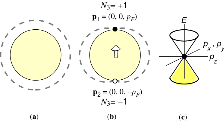
Figure 5: Angular dependence of the superfluid/superconducting gap (dashed lines) at the former Fermi surface (solid lines). The gap $\Delta$ is (a) isotropic in the $s$-wave state and (b) is $\Delta(\theta)=p_{F}c_{\perp}\sin\theta$ for the $p$-wave state in Eq.(16), where $\theta$ is the polar angle, and arrow shows the direction of the unit vector $\hat{\bf l}$. The spectrum of quasiparticles has two nodes at the former Fermi surface: at $\theta=0$, i.e. at ${\bf p}_{1}=p_{F}\hat{\bf l}$ (filled circle) and at $\theta=\pi$, i.e. at ${\bf p}_{2}=-p_{F}\hat{\bf l}$ (open circle). Their winding numbers of the Fermi points given by Eq.(17) are correspondingly $N_{3}=+1$ and $N_{3}=-1$. (c) According to Eq.(18), close to the Fermi points the quasiparticle spectrum becomes “relativistic”. For the local observer, who measures the spectrum using clocks and rods made of the low-energy fermions, the Hamiltonian for fermions in the vicinity of the point with $N_{3}=+1$ is equivalent to the Weyl Hamiltonian for the right handed massless fermions: $H=c{\mbox{\boldmath$\sigma$}}\cdot{\bf p}$; and the spectrum has the conical form $E=\pm cp$

The energy spectrum of these Bogoliubov–Nambu fermions is

$$E^{2}({\bf p})=\left({p^{2}\over 2m}-\mu\right)^{2}+\,c_{\perp}^{2}\,\left({\bf p}\times\hat{\bf l}\,\right)^{2}.$$ (16)

In the BCS regime occuring for positive chemical potential $\mu>0$, there are two Fermi points in 3D momentum space with $E({\bf p})=0$. For the energy spectrum (16), the Fermi points are ${\bf p}_{1}=p_{F}\,\hat{\bf l}$ and ${\bf p}_{2}=-p_{F}\,\hat{\bf l}$, with Fermi momentum $p_{F}=\sqrt{2m\mu}$ [Fig. 5(b)].

For a general system, be it relativistic or nonrelativistic, the topological stability of the Fermi point (the node of the co-dimension 3) is guaranteed by the nontrivial homotopy group $\pi_{2}(GL(n,{\bf C}))=Z$ which describes the mapping of a sphere $S^{2}$ embracing the point node to the space of non-degenerate complex matrices Horava . This is the group of integers. The integer valued topological invariant (winding number) can be written in terms of the fermionic propagator $G(i\omega,{\bf p})$ as a surface integral in the 4D frequency-momentum space $p_{\mu}=(\omega,{\bf p})$: VolovikBook

$$N_{3}\equiv{1\over{24\pi^{2}}}\,\epsilon_{\mu\nu\rho\sigma}~{}{\rm tr}\,\oint_{\Sigma_{a}}dS^{\sigma}G\frac{\partial}{\partial p_{\mu}}G^{-1}\;G\frac{\partial}{\partial p_{\nu}}G^{-1}\;G\frac{\partial}{\partial p_{\rho}}G^{-1}.$$ (17)

Here $\Sigma_{a}$ is a three-dimensional surface around the isolated Fermi point $p_{\mu a}=(0,{\bf p}_{a})$ and ‘tr’ stands for the trace over the relevant spin and/or band indices. For the case considered in Eq.(15), the Green’s function is $G^{-1}(i\omega,{\bf p})=i\omega-H({\bf p})$; the trace is over the Bogoliubov-Nambu spin; and the two Fermi points ${\bf p}_{1}$ and ${\bf p}_{2}$ have nonzero topological charges $N_{3}=+1$ and $N_{3}=-1$ [Fig. 6 (right)].

We call such Fermi points the chiral Fermi points, because in the vicinity of these point the fermions behave as right-handed or left handed particles (see below). These nodes of co-dimension 3 are the diabolical points – the exceptional degeneracy points of the complex-valued Hamiltonian which depends on the external parameters (see Ref. NeumannWigner ; StoneA ; Arnold ; Berry ). At these points two different branches of the spectrum touch each other. Topology of these points has been discussed in Ref. Novikov . In our case the relevant parameters of the Hamiltonian are the components of momentum ${\bf p}$, and we discuss the contact point of branches with positive and negative energies VolovikDiabolic . Topology of the chiral Fermi points in relation to the spectrum of elementary particles has been discussed in Ref. NielsenNinomiya .

Emergent relativity and chiral fermions

Close to any of the Fermi points the energy spectrum of fermionic quasiparticles acquires the relativistic form (this follows from the so-called Atiyah-Bott-Shapiro construction Horava ). In particular, the Hamiltonian in Eq.(15) and spectrum in Eq.(16) become VolovikBook :

$$H\rightarrow e_{k}^{i}\sigma^{k}(p_{i}-eA_{i})~{}~{},~{}~{}E^{2}({\bf p})\rightarrow g^{ik}(p_{i}-eA_{i})(p_{k}-eA_{k})~{}.$$ (18)

Here the analog of the dynamic gauge field is ${\bf A}=p_{F}\hat{\bf l}$; the “electric charge” is either $e=+1$ or $e=-1$ depending on the Fermi point; the matrix $e_{i}^{k}$ is the analog of the dreibein with $g^{ik}=e^{i}_{j}e^{k}_{j}={\rm diag}(c_{\perp}^{2},c_{\perp}^{2},c_{\parallel}^{2}=p_{F}^{2}/m^{2})$ playing the role of the effective dynamic metric in which fermions move along the geodesic lines. Fermions in Eq.(18) are chiral: they are right-handed if the determinant of the matrix $e^{i}_{j}$ is positive, which occurs at $N_{3}=+1$; the fermions are left-handed if the determinant of the matrix $e^{i}_{j}$ is negative, which occurs at $N_{3}=-1$. For the local observer, who measures the spectrum using clocks and rods made of the low-energy fermions, the Hamiltonian in Eq.(18) is simplified: $H=\pm c{\mbox{\boldmath$\sigma$}}\cdot{\bf p}$ [Fig. 5(c). Thus the chirality is the property of the behavior in the low energy corner and it is determined by the topological invariant $N_{3}$.

Majorana Fermi point

The Hamiltonians which give rise to the chiral Fermi points with non-zero $N_{3}$ are essentially complex matrices. That is why one may expect that in systems described by real-valued Hamiltonian matrices there are no topologically stable points of co-dimension 3. However, the general analysis in terms of $K$-theory Horava demonstrates that such points exist and are described by the group $Z_{2}$. Let us denote this $Z_{2}$ charge as $N_{3{\rm M}}$ to distinguish it from the $Z$ charge $N_{3}$ of chiral fermions. The summation law for the charge $N_{3{\rm M}}$ is $1+1=0$, i.e. two such points annihilate each other. Example of topologically stable massless real fermions is provided by the Majorana fermions Horava . The summation law $1+1=0$ also means that $1=-1$, i.e. the particle is its own antiparticle. This property of the Majorana fermions follows from the topology in momentum space and does not require the relativistic invariance.

Summation law for Majorana fermions and marginal Fermi point

The summation law $1-1=0$ for chiral fermions and $1+1=0$ for Majorana fermions is illustrated using the following $4\times 4$ Hamiltonian matrix:

$$H=c\tau_{1}p_{x}+c\tau_{2}\sigma_{2}p_{y}+c\tau_{3}p_{z}~{}.$$ (19)

This Hamiltonian describes either two chiral fermions or two Majorana fermions. The first description is obtained if one chooses the spin quantization axis along $\sigma_{2}$. Then for the direction of spin $\sigma_{2}=+1$ this Hamiltonian describes the right-handed fermion with spectrum $E(p)=cp$ whose Fermi point at ${\bf p}=0$ has topological charge $N_{3}=+1$. For $\sigma_{2}=-1$ one has the left-handed chiral fermion whose Fermi point is also at ${\bf p}=0$, but it has the opposite topological charge $N_{3}=-1$. Thus the total topological charge of the Fermi point at ${\bf p}=0$ is $N_{3}=1-1=0$.

In the other description, one takes into account that the matrix (19) is real and thus can describe the real (Majorana) fermions. In our case the original fermions are complex, and thus we have two real fermions with the spectrum $E(p)=cp$ representing the real and imaginary parts of the complex fermion. Each of the two Majorana fermions has the Fermi (Majorana) point at ${\bf p}=0$ where the energy of fermions is zero. Since the Hamiltonian (19) is the same for both real fermions, the two Majorana points have the same topological charge.

Let us illustrate the difference in the summation law for charges $N_{3}$ and $N_{3{\rm M}}$ by introducing the perturbation $M\sigma_{1}\tau_{2}$ to the Hamiltonian (19):

$$H=c\tau_{1}p_{x}+c\tau_{2}\sigma_{2}p_{y}+c\tau_{3}p_{z}+M\sigma_{1}\tau_{2}~{}.$$ (20)

Due to this perturbation the spectrum of fermions is fully gapped: $E^{2}(p)=c^{2}p^{2}+M^{2}$. In the description in terms of the chiral fermions, the perturbation mixes left and right fermions. This leads to formation of the Dirac mass $M$. The annihilation of Fermi points with opposite charges illustrates the summation law $1-1=0$ for the topological charge $N_{3}$.

Let us now consider the same process using the description in terms of real fermions. The added term $M\sigma_{1}\tau_{2}$ is imaginary. It mixes the real and imaginary components of the complex fermions, and thus it mixes two Majorana fermions. Since the two Majorana fermions have the same topological charge, $N_{3{\rm M}}=1$, the formation of the gap means that the like charges of the Majorana points annihilate each other. This illustrates the summation law $1+1=0$ for the Majorana fermions.

In both descriptions of the Hamiltonian (19), the total topological charge of the Fermi or Majorana point at ${\bf p}=0$ is zero. We call such topologically trivial point the marginal Fermi point. The topology does not protect the marginal Fermi point, and the small perturbation can lead to formation of the fully gapped vacuum, unless there is a symmetry which prohibits this.

3.2 Quantum phase transition in BCS–BEC crossover region

Splitting of marginal Fermi point

Let us consider some examples of quantum phase transition goverened by the momentum-space topology of gap nodes, between a fully-gapped vacuum state and a vacuum state with topologically-protected point nodes. In the context of condensed-matter physics, such a quantum phase transition may occur in a system of ultracold fermionic atoms in the region of the BEC–BCS crossover, provided Cooper pairing occurs in the non-$s$-wave channel. For elementary particle physics, such transitions are related to CPT violation, neutrino oscillations, and other phenomena SplittingPreprint .

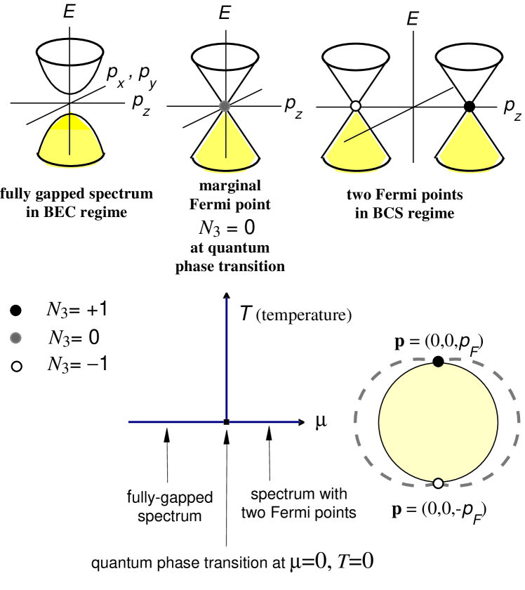
Figure 6: Quantum phase transition between two $p$-wave vacua with the same symmetry but of different universality class. In the bottom right corner you find the gap (dashed line) in the $p$-wave state. It depends on the direction in momentum space and becomes zero when ${\bf p}$ is along the $\hat{\bf l}$-vector (along $z$-axis). At $\mu>0$, two gap nodes give rise to two zeroes in the spectrum – Fermi points: one with winding number $N_{3}=+1$ (filled circle) and another with winding number $N_{3}=-1$ (open circle). The transition occurs when the chemical potential $\mu$ in Eq.(15) crosses zero value. The Fermi points merge at $\mu=0$ forming the marginal (topologically trivial) gap node with $N_{3}=0$ (grey circle) and annihilate each other. At $\mu<0$ the Green’s function has no singularities and the quantum vacuum is fully gapped

Let us start with the topological quantum phase transition involving topologically stable Fermi points Book1 ; QPT . Let us consider what happens with the Fermi points in Eq. (16), when one varies the chemical potential $\mu$. For $\mu>0$, there are two Fermi points, and the density of fermionic states in the vicinity of Fermi points is $\nu(\omega)\propto\omega^{2}$. For $\mu<0$, Fermi points are absent and the spectrum is fully-gapped [Fig. 6]. In this topologically-stable fully-gapped vacuum, the density of states is drastically different from that in the topologically-stable gapless regime: $\nu(\omega)=0$ for $\omega<|\mu|$. This demonstrates that the quantum phase transition considered is of purely topological origin. The transition occurs at $\mu=0$, when two Fermi points with $N_{3}=+1$ and $N_{3}=-1$ merge and form one topologically-trivial Fermi point with $N_{3}=0$, which disappears at $\mu<0$.

The intermediate state at $\mu=0$ is marginal: the momentum-space topology is trivial ($N_{3}=0$) and cannot protect the vacuum against decay into one of the two topologically-stable vacua unless there is a special symmetry which stabilizes the marginal node. As we shall see in the Sec. 3.3, the latter takes place in the Standard Model with marginal Fermi point.

Transition involving multiple nodes

The Standard Model contains 16 chiral fermions in each generation. The multiple Fermi point may occur in condensed matter too. For systems of cold atoms, an example is provided by another spin-triplet $p$–wave state, the so-called $\alpha$–phase. The Bogoliubov-Nambu Hamiltonian which qualitatively describes fermionic quasiparticles in the $\alpha$–state is given by VolovikGorkov1985 ; VollhardtWoelfle :

$$H=\left(\matrix{p^{2}/2m-\mu&\left({\bf\Sigma}\cdot{\bf p}\right)\,c_{\perp}/\sqrt{3}\cr\left({\bf\Sigma}\cdot{\bf p}\right)^{\dagger}\,c_{\perp}/\sqrt{3}&-p^{2}/2m+\mu\cr}\right),$$ (21)

with ${\bf\Sigma}\cdot{\bf p}\equiv\sigma_{x}p_{x}+\exp(2\pi i/3)\,\sigma_{y}p_{y}+\exp(-2\pi i/3)\,\sigma_{z}p_{z}\,$.

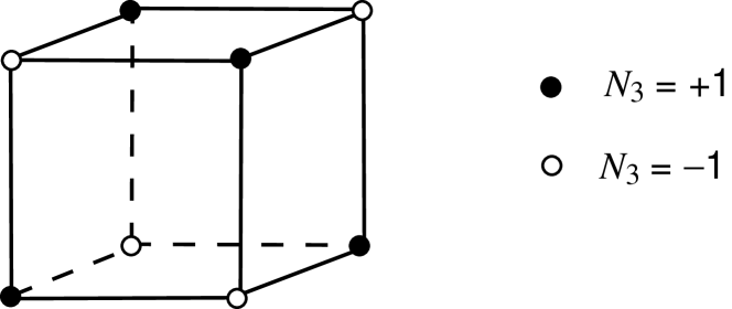
Figure 7: Fermi points in the $\alpha$-phase of triplet superfluid/superconductor in the BCS regime

On the BEC side ($\mu<0$), fermions are again fully-gapped, while on the BCS side ($\mu>0$), there are 8 topologically protected Fermi points with charges $N_{3}=\pm 1$, situated at the vertices of a cube in momentum space VolovikGorkov1985 [Fig. 7]. The fermionic excitations in the vicinity of these points are left- and right-handed Weyl fermions. At the transition point at $\mu=0$ these 8 Fermi points merge forming the marginal Fermi point at ${\bf p}=0$.

3.3 Quantum phase transitions in Standard Model

Marginal Fermi point in Standard Model

It is assumed that the Standard Model above the electroweak transition contains 16 chiral fermions in each generation: 8 right-handed fermions with $N_{3}=+1$ each and 8 left-handed fermions with $N_{3}=-1$ each. If so, then the vacuum of the Standard Model above the electroweak transition is marginal: there is a multiply degenerate Fermi point at ${\bf p}=0$ with the total topological charge $N_{3}=+8-8=0$ [Fig. 8(a)]. This vacuum is therefore the intermediate state between two topologically-stable vacua: the fully-gapped vacuum in Fig. 8(b); and the vacuum with topologically-nontrivial Fermi points in Fig. 8(c).

The absence of the topological stability means that even the small mixing between the fermions leads to annihilation of the Fermi point. In the Standard Model, the proper mixing which leads to the fully gapped vacuum is prohibited by symmetries, namely the continuous electroweak $U(1)\times SU(2)$ symmetry (or the discrete symmetry discussed in Sec. 12.3.2 of Ref.VolovikBook ) and the CPT symmetry. (Marginal gapless fermions emerging in spin systems were discussed in WenPRL . These massless Dirac fermions protected by symmetry differ from the chiral fermions of the Standard Model. The latter cannot be represented in terms of massless Dirac fermions, since there is no symmetry between left and right fermions in Standard Model.)

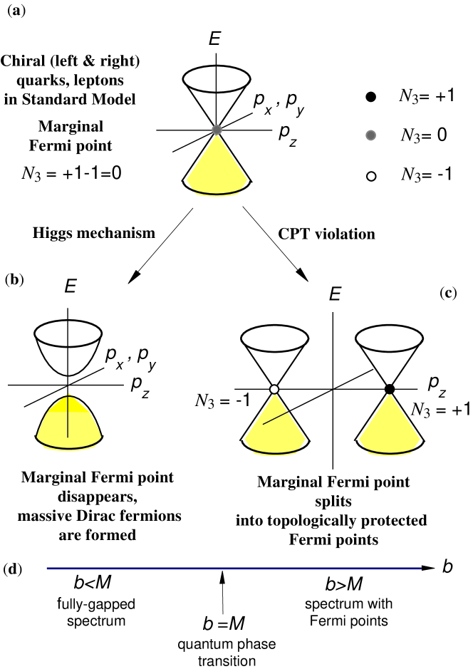
Figure 8: Two scenarios of annihilation of marginal Fermi point (a) in Standard Model of strong and electroweak interactions. Higgs mechanism leads to Dirac mass and thus to the fully gapped vacuum (b), while CPT violation leads to splitting of Fermi points (c). In the bottom edge you find the quantum phase transition in the model in Eq.(25) when the CPT violating parameter $b\equiv|{\bf b}|$ crosses the Dirac mass $M$

Explicit violation or spontaneous breaking of electroweak or CPT symmetry transforms the marginal vacuum of the Standard Model into one of the two topologically-stable vacua. If, for example, the electroweak symmetry is broken, the marginal Fermi point disappears and the fermions become massive [Fig. 8(b)]. This is assumed to happen below the symmetry breaking electroweak transition caused by Higgs mechanism where quarks and charged leptons acquire the Dirac masses. If, on the other hand, the CPT symmetry is violated, the marginal Fermi point splits into topologically-stable Fermi points which protect chiral fermions [Fig. 8(c)]. One can speculate that in the Standard Model the latter happens with the electrically neutral leptons, the neutrinos SplittingPreprint ; KlinkhamerCPT .

Quantum phase transition with splitting of Fermi points

Let us consider this scenario on a simple example of a marginal Fermi point describing a single pair of relativistic chiral fermions, that is, one right-handed fermion and one left-handed fermion. These are Weyl fermions with Hamiltonians $H_{\rm right}={\mbox{\boldmath$\sigma$}}\cdot{\bf p}$ and $H_{\rm left}=-{\mbox{\boldmath$\sigma$}}\cdot{\bf p}$, where $\sigma$ denotes the triplet of spin Pauli matrices. Each of these Hamiltonians has a topologically-stable Fermi point at ${\bf p}=0$. The corresponding inverse Green’s functions are given by

$$G^{-1}_{\rm right}(i\omega,{\bf p}) = i\omega-{\mbox{\boldmath$\sigma$}}\cdot{\bf p}\;,$$ (22)

$$G^{-1}_{\rm left}(i\omega,{\bf p}) = i\omega+{\mbox{\boldmath$\sigma$}}\cdot{\bf p}~{}.$$ (23)

The positions of the Fermi points coincide, ${\bf p}_{1}={\bf p}_{2}=0$, but their topological charges (17) are different. For this simple case, the topological charge equals the chirality of the fermions, $N_{3}=C_{a}$ (i.e., $N_{3}=+1$ for the right-handed fermion and $N_{3}=-1$ for the left-handed one). The total topological charge of the Fermi point at ${\bf p}=0$ is therefore zero.

The splitting of this marginal Fermi point can be described by the Hamiltonians $H_{\rm right}={\mbox{\boldmath$\sigma$}}\cdot({\bf p}-{\bf p}_{1})$ and $H_{\rm left}=-{\mbox{\boldmath$\sigma$}}\cdot({\bf p}-{\bf p}_{2})$, with ${\bf p}_{1}=-{\bf p}_{2}\equiv{\bf b}$ from momentum conservation. The real vector ${\bf b}$ is assumed to be odd under CPT, which introduces CPT violation into the physics. The $4\times 4$ matrix of the combined Green’s function has the form

$$G^{-1}(i\omega,{\bf p})=\left(\matrix{i\omega-{\mbox{\boldmath$\sigma$}}\cdot({\bf p}-{\bf b})&0\cr 0&i\omega+{\mbox{\boldmath$\sigma$}}\cdot({\bf p}+{\bf b})\cr}\right).$$ (24)

Equation  (17) shows that ${\bf p}_{1}={\bf b}$ is the Fermi point with topological charge $N_{3}=+1$ and ${\bf p}_{2}=-{\bf b}$ the Fermi point with topological charge $N_{3}=-1$.

Let us now consider the more general situation with both the electroweak and CPT symmetries broken. Due to breaking of the electroweak symmetry the Hamiltonian acquires the off-diagonal term (mass term) which mixes left and right fermions

$$H=\left(\matrix{{\mbox{\boldmath$\sigma$}}\cdot({\bf p}-{\bf b})&M\cr M&-{\mbox{\boldmath$\sigma$}}\cdot({\bf p}+{\bf b})\cr}\right)~{}.$$ (25)

The energy spectrum of Hamiltonian (25) is

$$E^{2}_{\pm}({\bf p})=M^{2}+|{\bf p}|^{2}+b^{2}\pm\,2\,b\,\sqrt{M^{2}+\left({\bf p}\cdot\hat{{\bf b}}\right)^{2}}~{},$$ (26)

with $\hat{{\bf b}}\equiv{\bf b}/|{\bf b}|$ and $b\equiv|{\bf b}|$.

Allowing for a variable parameter $b$, one finds a quantum phase transition at $b=M$ between the fully-gapped vacuum for $b<M$ and the vacuum with two isolated Fermi points for $b>M$ [Fig. 8(d)]. These Fermi points are situated at

$${\bf p}_{1} = +\hat{{\bf b}}\;\sqrt{b^{2}-M^{2}}\;,$$ (27)

$${\bf p}_{2} = -\hat{{\bf b}}\;\sqrt{b^{2}-M^{2}}~{}.$$ (28)

Equation  (17), now with a trace over the indices of the $4\times 4$ Dirac matrices, shows that the Fermi point at ${\bf p}_{1}$ has topological charge $N_{3}=+1$ and thus the right-handed chiral fermions live in the vicinity of this point. Near the Fermi point at ${\bf p}_{2}$ with the charge $N_{3}=-1$, the left-handed fermions live. The magnitude of the splitting of the two Fermi points is given by $2\,\sqrt{b^{2}-M^{2}}\,$. At the quantum phase transition $b=M$, the Fermi points with opposite charge annihilate each other and form a marginal Fermi point at ${\bf p}=0$. The momentum-space topology of this marginal Fermi point is trivial (the topological invariant $N_{3}=+1-1=0$).

Fermi surface with global charge $N_{3}$ and quantum phase transition with transfer of $N_{3}$

Extension of the model (25) by introducing the time like parameter $b_{0}$

$$H=\left(\matrix{{\mbox{\boldmath$\sigma$}}\cdot({\bf p}-{\bf b})-b_{0}&M\cr M&-{\mbox{\boldmath$\sigma$}}\cdot({\bf p}+{\bf b})+b_{0}\cr}\right)~{},$$ (29)

demonstrates another type of quantum phase transitions SplittingPreprint shown in Fig. 9.

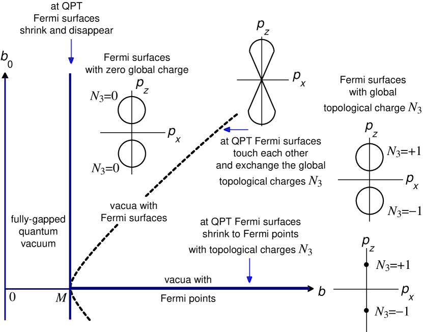
Figure 9: Topological quantum phase transitions in the model (29). The vacua at $b_{0}\neq 0$ and $b>M$ have Fermi surfaces. At $b^{2}>b_{0}^{2}+M^{2}$, these Fermi surfaces have nonzero global topological charges $N_{3}=+1$ and $N_{3}=-1$. At the quantum phase transition occurring on the line $b_{0}=0$, $b>M$ (thick horizontal line) the Fermi surfaces shrink to the Fermi points with nonzero $N_{3}$. At $M^{2}<b^{2}<b_{0}^{2}+M^{2}$ the global topology of the Fermi surfaces is trivial, $N_{3}=0$. At the quantum phase transition occurring on the line $b=M$ (thick vertical line), the Fermi surfaces shrink to the points; and since their global topology is trivial the zeroes disappear at $b<M$ where the vacuum is fully gapped. The quantum phase transition between the Fermi surfaces with and without topological charge $N_{3}$ occurs at $b^{2}=b_{0}^{2}+M^{2}$ (dashed line). At this transition, the Fermi surfaces touch each other, and their topological charges annihilate each other

At $b_{0}\neq 0$, Fermi points which exist at $b_{0}=0$, $b>M$ transform to the closed Fermi surfaces. These Fermi surfaces in addition to the local charge $N_{1}$ have the global topological invariant $N_{3}$ inherited from the original Fermi points. The global charge $N_{3}$ is defined by the same Eq. (17), but with a three-dimensional surface $\Sigma_{a}$ around the whole Fermi surface. On the line of the quantum phase transition, $b^{2}-b_{0}^{2}=M^{2}$ (dashed line), two Fermi surfaces contact each other at the point ${\bf p}=0$. At that moment, the topological charge $N_{3}$ is transferred between the Fermi surfaces through the point of the contact. Above the transition line, the global charges of Fermi surfaces are zero. At the quantum phase transition at $b=M$ (thick vertical line) these Fermi surfaces shrink to the points; and since the $N_{3}$ topology of these points is trivial they disappear at $b<M$ where the state is fully gapped.

Standard Model with chiral Fermi point

In the above consideration we assumed that the Fermi point in the Standard Model above the electroweak energy scale is marginal, i.e. its total topological charge is $N_{3}=0$. Since the topology does not protect such a point, everything depends on symmetry, which is a more subtle issue. In principle, one may expect that the vacuum is always fully gapped. This is supported by the Monte-Carlo simulations which suggest that in the Standard Model there is no second-order phase transition at finite temperature, instead one has either the first-order electroweak transition or crossover depending on the ratio of masses of the Higgs and gauge bosons Kajantie . This would actually mean that the fermions are always massive.

Such scenario does not contradict to the momentum-space topology, only if the total topological charge $N_{3}$ is zero. However, from the point of view of the momentum-space topology there is another scheme of the description of the Standard Model. Let us assume that the Standard Model follows from the GUT with $SO(10)$ group. In this scheme, the 16 Standard Model fermions form at high energy the 16-plet of the $SO(10)$ group. All the particles of this multiplet are left-handed fermions. These are: four left-handed $SU(2)$ doublets (neutrino-electron and 3 doublets of quarks) + eight left $SU(2)$ singlets of anti-particles (antineutrino, positron and 6 anti-quarks). The total topological charge of the Fermi point at ${\bf p}=0$ is $N_{3}=-16$, and thus such a vacuum is topologically stable and is protected against the mass of fermions. This topological protection works even if the $SU(2)\times U(1)$ symmetry is violated perturbatively, say, due to the mixing of different species of the 16-plet. Mixing of left leptonic doublet with left singlets (antineutrino and positron) violates $SU(2)\times U(1)$ symmetry, but this does not lead to annihilation of Fermi points and mass formation since the topological charge $N_{3}$ is conserved.

We discussed the similar situation in the Sec. 2.3 for the case of the Fermi surface, and found that if the total topological charge of the Fermi surfaces is non-zero, the gap cannot appear perturbatively. It can only arise due to the crucial reconstruction of the fermionic spectrum with effective doubling of fermions. In the same manner, in the $SO(10)$ GUT model the mass generation can only occur non-perturbatively. The mixing of the left and right fermions requires the introduction of the right fermions, and thus the effective doubling of the number of fermions. The corresponding Gor’kov’s Green’s function in this case will be the $(16\times 2)\times(16\times 2)$ matrix. The nullification of the topological charge $N_{3}=-16$ occurs exactly in the same manner, as in superconductors. In the extended (Gor’kov) Green’s function formalism appropriate below the transition, the topological charge of the original Fermi point is annihilated by the opposite charge $N_{3}=+16$ of the Fermi point of ‘holes’ (right-handed particles).

This demonstrates that the mechanism of generation of mass of fermions essentially depends on the momentum space topology. If the Standard Model originates from the $SO(10)$ group, the vacuum belongs to the universality class with the topologically non-trivial chiral Fermi point (i.e. with $N_{3}\neq 0$), and the smooth crossover to the fully-gapped vacuum is impossible. On the other hand, if the Standard Model originates from the left-right symmetric Pati-Salam group such as $SU(2)_{L}\times SU(2)_{R}\times SU(4)$, and its vacuum has the topologically trivial (marginal) Fermi point with $N_{3}=0$, the smooth crossover to the fully-gapped vacuum is possible.

Chiral anomaly

Since chiral Fermi points in condensed matter and in Standard Model are described by the same momentum-space topology, one may expect common properties. An example of such a common property would be the axial or chiral anomaly. For quantum anomalies in (3+1)–dimensional systems with Fermi points and their dimensional reduction to (2+1)–dimensional systems, see, e.g., Ref. VolovikBook and references therein. In superconducting and superfluid fermionic systems the chiral anomaly is instrumental for the dynamics of vortices. In particular, one of the forces acting on continuous vortex-skyrmions in superfluid ³He-A is the result the anomalous production of the fermionic charge from the vacuum decsribed by the Adler-Bell-Jackiw equation Adler .

4 Fermi lines

In general the zeroes of co-dimension 2 (nodal lines in 3D momentum space or point nodes in 2D momentum space) do not have the topological stability. However, if the Hamiltonian is restricted by some symmetry, the topological stability of these nodes is possible. The nodal lines do not appear in spin-triplet superconductors, but they may exist in spin-singlet superconductors VolovikGorkov1985 ; Blount . The analysis of topological stability of nodal lines in systems with real fermions was done by Horava Horava .

4.1 Nodes in high-$T_{c}$ superconductors

An example of point nodes in 2D momentum space is provided by the layered quasi-2D high-T_c superconductor. In the simplest form, omitting the mass and the amplitude of the order parameter, the 2D Bogoliubov-Nambu Hamiltonian is

$$H=\tau_{3}\left(\frac{p_{x}^{2}+p_{y}^{2}}{2m}-\mu\right)+a\tau_{1}(p_{x}^{2}-\lambda p_{y}^{2})~{}.$$ (30)

In case of tetragonal crystal symmetry one has either the pure $s$-wave state with $\lambda=-1$ ($p_{x}^{2}+p_{y}^{2}$) or the pure $d$-wave state with $\lambda=+1$ ($p_{x}^{2}-p_{y}^{2}$). But in case of orthorhombic crystal these two states are not distinguishible by symmetry and thus the general order parameter is represented by the $s+d$ combination, i.e. in the orthorhombic crystal one always has $|\lambda|\neq 1$. For example, experiments in high-T_c cuprate YBa₂Cu₃O₇ suggest that $\lambda\sim 0.7$ in this compound AnisotropyExperiment .

At $\mu>0$ and $\lambda>0$, the energy spectrum contains 4 point nodes in 2D momentum space (or four Fermi-lines in the 3D momentum space):

$$p_{x}^{a}=\pm p_{F}\sqrt{\lambda\over 1+\lambda}~{}~{},~{}~{}p_{y}^{a}=\pm p_{F}\sqrt{1\over 1+\lambda}~{}~{},~{}~{}p_{F}^{2}=2\mu~{}.$$ (31)

The problem is whether these nodes survive or not if we extend Eq.(30) to the more general Hamiltonian obeying the same symmetry. The important property of this Hamiltonian is that, as distinct from the Hamiltonian (15), it obeys the time reversal symmetry which prohibits the imaginary $\tau_{2}$-term. In the spin singlet states the Hamiltonian obeying the time reversal symmetry must satisfy the equation $H^{*}(-{\bf p})=H({\bf p})$. The general form of the $2\times 2$ Bogoliubov-Nambu spin-singlet Hamiltonian satisfying this equation can be expressed in terms of the 2D vector ${\bf m}({\bf p})=(m_{x}({\bf p}),m_{y}({\bf p}))$:

$$H=\tau_{3}m_{x}({\bf p})+\tau_{1}m_{y}({\bf p})~{}.$$ (32)

Using this vector one can construct the integer valued topological invariant – the contour integral around the point node in 2D momentum space or around the nodal line in 3D momentum space:

$$N_{2}=\frac{1}{2\pi}\oint dl~{}\hat{\bf z}\cdot\left(\hat{\bf m}\times\frac{d\hat{\bf m}}{dl}\right)~{},$$ (33)

where $\hat{{\bf m}}\equiv{\bf m}/|{\bf m}|$. This is the winding number of the plane vector ${\bf m}({\bf p})$ around a vortex line in 3D momentum space or around a point vortex in 2D momentum space. The winding number is robust to any change of the Hamiltonian respecting the time reversal symmetry, and this is the reason why the node is stable.

All four nodes in the above example of Eq.(30) are topologically stable, since nodes with equal signs (++ and $--$) have winding number $N_{2}=+1$, while the other two nodes have winding number $N_{2}=-1$ [Fig. 11].

4.2 $Z_{2}$-lines

Now let us consider the stability of these nodes using the general topological analysis (the so-called $K$-theory, see Horava ). For the general $n\times n$ real matrices the classification of the topologically stable nodal lines in 3D momentum space (zeroes of co-dimension 2) is given by the homotopy group $\pi_{1}(GL(n,{\bf R}))$ Horava . It determines classes of mapping of a contour $S^{1}$ around the nodal line (or around a point in the 2D momentum space) to the space of non-degenerate real matrices. The topology of nodes depends on $n$. If $n=2$, the homotopy group for lines of nodes is $\pi_{1}(GL(2,{\bf R}))=Z$, it is the group of integers in Eq.(33) obeying the conventional summation $1+1=2$. However, for larger $n\geq 3$ the homotopy group for lines of nodes is $\pi_{1}(GL(n,{\bf R}))=Z_{2}$, which means that the summation law for the nodal lines is now $1+1=0$, i.e. two nodes with like topological charges annihilate each other. These nodes of co-dimension 2 are similar to the points of degeneracy of the energy spectrum of the real-valued Hamiltonian which depends on the external parameters (see Ref. NeumannWigner ; Arnold ; Berry ).

The equation (30) is the $2\times 2$ Hamiltonian for the complex fermionic field. But each complex field consists of two real fermionic field. In terms of the real fermions, this Hamiltonian is the $4\times 4$ matrix and thus all the nodes must be topologically unstable. What keep them alive is the time reversal symmetry, which does not allow to mix real and imaginary components of the complex field. As a result, the two components are independent; they are described by the same $2\times 2$ Hamiltonian (30); they have zeroes at the same points; and these zeroes are described by the same topological invariants.

If we allow mixing between real and imaginary components of the spinor by introducing the imaginary perturbation to the Hamiltonian, such as $M\tau_{2}$, the summation law $1+1$ leads to immediate annihilation of the zeroes situated at the same points. As a result the spectrum becomes fully gapped:

$$E^{2}({\bf p})=\left(\frac{p_{x}^{2}+p_{y}^{2}}{2m}-\mu\right)^{2}+a^{2}(p_{x}^{2}-\lambda p_{y}^{2})^{2}+M^{2}~{}.$$ (34)

Thus to destroy the nodes of co-dimension 2 occurring for $2\times$ real-valued Hamiltonian (30) describing complex fermions it is enough to violate the time reversal symmetry.

How to destroy the nodes if the time reversal symmetry is obeyed which prohibits mixing? One possibility is to deform the order parameter in such a way that the nodes with opposite $N_{2}$ merge and then annihilate each other forming the fully gapped state. In this case, at the border between the state with nodes and the fully gapped state the quantum phase transition occurs (see Sec. 4.7). This type of quantum phase transition which involves zeroes of co-dimension 2 was also discussed in Ref.WenZee .

Another possibility is to increase the dimension of the matrix from $2\times 2$ to $4\times 4$. Let us consider this case.

4.3 Gap induced by interaction between layers

High-$T_{c}$ superconductors typically have several superconducting cuprate layers per period of the lattice, that is why the consideration of two layers which are described by $4\times 4$ real Hamiltonians is well justified. Let us start again with $2\times 2$ real matrix $H$, and choose for simplicity the easiest form for the vector ${\bf m}({\bf p})$. For ${\bf m}({\bf p})={\bf p}=(p_{x},p_{y})$ the Hamiltonian is

$$H=\tau_{3}p_{x}+\tau_{1}p_{y}~{}.$$ (35)

The node which we are interested in is at $p_{x}=p_{y}=0$ and has the topological charge (winding number) $N_{2}=1$ in Eq.(33). The Dirac-type Hamiltonian (35) and the corresponding nodes of co-dimension 2 are relevant for electrons leaving in the 2D carbon sheet known as graphene Novoselov ; Gusynin ; NovoselovQHE ; Falko .

Let us now introduce two bands or layers whose Hamiltonians have opposite signs:

$$H_{11}=\tau_{3}p_{x}+\tau_{1}p_{y}~{}~{},~{}~{}H_{22}=-\tau_{3}p_{x}-\tau_{1}p_{y}~{},$$ (36)

Each Hamiltonian has a node at $p_{x}=p_{y}=0$. In spite of the different signs of the Hamiltonian, the nodes have same winding number $N_{2}=1$: in the second band one has ${\bf m}_{2}({\bf p})=-{\bf m}_{1}({\bf p})$, but $N_{2}({\bf m})=N_{2}(-{\bf m})$ according to Eq.(33).

The Hamiltonians (35) and (36) can be now combined in the $4\times 4$ real Hamiltonian:

$$H=\sigma_{3}(\tau_{3}p_{x}+\tau_{1}p_{y})~{},$$ (37)

where $\sigma$ matrices operate in the 2-band space. The Hamiltonian (37) has two nodes: one is for projection $\sigma_{3}=1$ and another one – for the projection $\sigma_{3}=-1$. Their positions in momentum space and their topological charges coincide. Let us now add the term with $\sigma_{1}$, which mixes the two bands without violation of the time reversal symmetry:

$$H=\sigma_{3}(\tau_{3}p_{x}+\tau_{1}p_{y})+\sigma_{1}m~{}.$$ (38)

The spectrum becomes fully gapped, $E^{2}=p^{2}+m^{2}$, i.e. the two nodes annililate each other. Since the nodes have the same winding number $N_{2}$, this means that the summation law for these nodes is 1+1=0. Thus the zeroes of co-dimension 2 (nodal points in 2D systems or the nodal lines in the 3D systems) which appear in the $4\times 4$ (and higher) real Hamiltonians are described by the $Z_{2}$-group. The discussion of the $Z_{2}$ nodes in high-$T_{c}$ materials, polar state of $p$-wave pairing and mixed singlet-triplet superconducting states can be found in Ref. Sato .

4.4 Gap vs splitting of nodes in bilayer materials

The above example demonstrated how in the two band systems (or in the double layer systems) the interaction between the bands (layers) induces the annihilation of likewise nodes and formation of the fully gapped state. Experiments on the graphite film with two graphene layers demonstrate that the spectrum of quasiparticles is essentially different from that in a single carbon sheet NovoselovQHE . From the detailed calculations Falko it follows that the gap in the spectrum emerges in the graphite bilayer at the neutrality point, illustrating the rule $1+1=0$ for the $Z_{2}$ nodes of co-dimension 2.

Applying this to the high-T_c materials with 2, 3 or 4 cuprate layers per period, one concludes that the interaction between the layers can in principle induce a small gap even in a pure $d$-wave state. However, this does not mean that such destruction of the Fermi lines necessarily occurs. Instead, the interaction between the bands (layers) can lead to splitting of nodes, which then will occupy different positions in momentum space and thus cannot annihilate. Which of the two scenarios occurs – gap formation or splitting of nodes – depends on the parameters of the system. Changing these parameters one can produce the topological quantum phase transition from the fully gapped vacuum state to the vacuum state with pairs of nodes, as we discussed for the case of nodes with co-dimension 3 in Sec. 3. The splitting of nodes has been observed in the bilayer cuprate Bi₂Sr₂CaCu₂O_8+δ Kordyuk ; Ino . If in the other bilayer cuprates the splitting is not well resolved, this might be the indication of the small gap there.

4.5 Exotic fermions and reentrant violation of ‘special relativity’ in bilayer graphene

There still can be some discrete symmetry which forbids the annihilation of nodes of co-dimension 2, even if the nodes are not separated in momentum space. This is the symmetry between the two layers which forbids the rule $1+1=0$. For example, if the Hamiltonian still anti-commutes with some matrix, say, with $\tau_{2}$-matrix, there is a generalization of the integer valued invariant in Eq.(33) to the $2n\times 2n$ real Hamiltonian (see also WenZee ):

$$N_{2}=-{1\over 4\pi i}~{}{\rm tr}~{}\oint dl~{}\tau_{2}H^{-1}\nabla_{l}H~{}.$$ (39)

Since the summation law for this $N_{2}$ charge is 1+1=2, the nodes with $N_{2}=1$ present at each layer do not annihilate each other if the interaction term preserves the symmetry. In this case the spectrum of the bilayer system remains gapless.

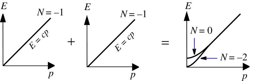
Figure 10: Reentrant violation of special relativity in 2D and 3D systems. Close to the topologically stable zero, single fermion has a relativistic spectrum. $N$ stands for the topological charge $N_{2}$ in 2D systems and the topological charge $N_{3}$ for 3D systems. In case of several relativistic fermions with the same topological charge, the interaction between the fermions may lead to the rearrangement of the topological charges between the fermions, $(-1)+(-1)\rightarrow(-2)+0$. This means that mixing between two left-handed neutrinos with charges $N_{3}=-1$ each results in one exotic non-relativistic neutrino with $N_{3}=-2$ and one massive neutrino with $N_{3}=0$. The same occurs for the fermions in the bilayer graphene, $1+1\rightarrow 2+0$: due to interaction between the layers, two Dirac fermions (one per each layer) with spectrum $E=cp$ transform to one exotic non-relativistic fermion with $N_{2}=2$ and quadratic spectrum $p^{2}/2m$ and one fully gapped fermion with $N_{2}=0$.

Let us now consider the gapless spectrum in such bilayer material. We start again with the Hamiltonian in Eq.(37), which describes gapless Dirac quasiparticles living in two independent layers, and add the interaction between them which does not violate the $\tau_{2}$-symmetry:

$$H=\sigma_{3}(\tau_{3}p_{x}+\tau_{1}p_{y})+m(\tau_{1}\sigma_{1}-\tau_{3}\sigma_{2})~{}.$$ (40)

The energy spectrum becomes

$$E_{+}=\pm\left(\sqrt{m^{2}+p^{2}}+m\right)~{}~{},~{}~{}E_{-}=\pm\left(\sqrt{m^{2}+p^{2}}-m\right)~{}.$$ (41)

Without interaction, i.e. at $m=0$, the quasiparticles represent two Dirac fermions with the topological charges $N_{2}=1$ each. Since the Hamiltonian (40) anti-commutes with the $\tau_{2}$-matrix, the total topological charge $N_{2}$ must be conserved even at $m\neq 0$. Thus the total charge for quasiparticles must be $N_{2}=2$. However it is now distributed between the branches of quasiparticle spectrum in the following manner (Fig. 10). For $m>0$, the quasiparticles with energy $E_{+}$ acquire the trivial topological charge $N_{2}=0$, that is why their spectrum becomes fully gapped: $E_{+}(p\ll m)\approx\pm 2m$. The quasiparticles with energy $E_{-}$ have the rest nonzero topological charge $N_{2}=2$, and thus they must be gapless. The energy spectrum of these gapless fermions with $N_{2}=2$ is exotic: at $p\ll m$ the spectrum becomes that of classical particles with positive and negative masses, $E_{-}\approx\pm p^{2}/2m$; in the region $p\gg m$ it is relativistic $E\approx\pm p$; and finally the relativistic invariance is violated again at high $p$ of order of inverse inter-atomic distance. When the parameter $m$ crosses zero, the quantum phase transition occurs.

It is important that the exotic branch with $N_{2}=2$ contains only single fermionic species, i.e. it cannot split into two fermions with $N_{2}=1$ each. That is why the quadratic law for the spectrum of exotic fermions is generic, provided that the proper symmetry of the Hamiltonian is obeyed. The same spectrum (41) takes place for quasiparticles in the carbon film consisting of two graphene sheets: it occurs in some range of parameters of the system where terms in the Hamiltonian, which violate the $\tau_{2}$-symmetry and induce the gap in the spectrum, are small and can be neglected Falko . Exotic fermions with parabolic spectrum lead to the unconventional quantum Hall effect Falko , which has been observed in the bilayer graphene NovoselovQHE .

All this shows that the stability of and the summation law for the nodal lines depend on the type of discrete symmetry which protects the topological stability. The integer valued topological invariants protected by discrete or continuous symmetry were discussed in Chapter 12 of the book VolovikBook .

If the symmetry is obeyed we have the following situation. Fermions with the elementary topological charge, $N_{2}=\pm 1$, are necessarily relativistic in the low-energy corner, according to the Atiyah-Bott-Shapiro construction. However, even a very small interaction between two species with $N_{2}=+1$ each may produce the exotic fermions, which are classical. In this scenario the Lorentz invariance is violated both at very high and at very low energies, therefore the term ‘reentrant violation of special relativity’.

4.6 Reentrant violation of special relativity in 3D systems

Similar reentrant violation of Lorentz invariance in the 3D vacua may occur for the Fermi points of co-dimension 3 described by the topological charge $N_{3}$ VolovikReentrant ; VolovikBook . Let us suppose that the Standard Model is an effective theory, and that the right-handed neutrinos are absent in this theory. The left-handed neutrino, which has $N_{3}=-1$, is necessarily massless. Its spectrum is necessarily relativistic in the low-energy corner, and thus the Lorentz invariance emerges at low energies. However, according to the general rules, if several species of the left-handed neutrino are present, so that $|N_{3}|>1$, the necessary violation of the Lorentz invariance at high energy must induce the violation of the Lorentz invariance at very low energy. Let us consider the case of two flavors of the left-handed neutrino – electron and muon neutrinos with $N_{3}=-1$ each in Fig. 10 (left). If the Standard Model is an effective theory, the high-energy cut-off induces mixing between the two flavors. The mixing is rather small, since it contains the high-energy cut-off in the denominator. Such a mixing typically leads to the rearrangement of the topological charges: $(-1)+(-1)\rightarrow(-2)+0$. This means that the two chiral neutrinos transform into one exotic non-relativistic neutrino with $N_{3}=-2$ and one massive neutrino with $N_{3}=0$ in Fig. 10 (right). In the particular model discussed in Refs. VolovikReentrant ; VolovikBook , the corresponding spectrum of two neutrino flavors is

$$E_{\pm}^{2}=p_{z}^{2}+\left(\sqrt{m^{2}+p_{x}^{2}+p_{y}^{2}}\pm m\right)^{2}~{}.$$ (42)

At $p_{z}=0$, this 3D spectrum transforms to the 2D spectrum in Eq.(41). The magnitude $m$ of the splitting of the neutrino spectrum has been discussed in Ref. KlinkhamerReentrant . Some speculations on the possible consequences of the reentrant violation of special relativity are discussed in Ref. Consoli .

4.7 Quantum phase transition in high-T_c superconductor

Let us return to the $2\times 2$ real Hamiltonian (30) and consider what happens with gap nodes when one changes the asymmetry parameter $\lambda$. When $\lambda$ crosses zero there is a quantum phase transition at which nodes in the spectrum annihilate each other and then the fully gapped spectrum develops [Fig. 11]. Note that there is no symmetry change across the phase transtion.

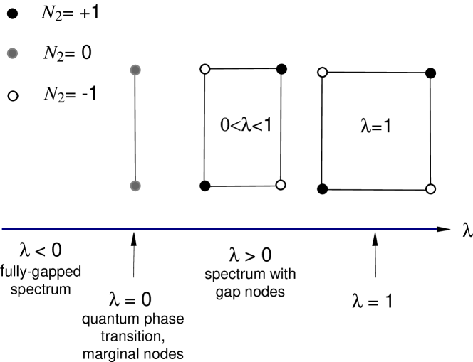
Figure 11: Quantum phase transition by change of anisotropy parameter $\lambda$ in Eq. (30) for superconductors in the $d+s$ state. At $\lambda>0$ the 2D spectrum has 4 nodes: two with topological charge $N_{2}=+1$ (filled circles) and two with topological charge $N_{2}=-1$ (open circles). At $\lambda=0$, points with opposite charges merge forming two marginal nodes with $N_{2}=0$ (grey circles). The marginal (topologically trivial) nodes disappear at $\lambda<0$ leaving the fully gapped vacuum

The similar quantum phase transition from gapless to gapped state without change of symmetry also occurs when $\mu$ crosses zero. This scenario can be realized in the BEC–BCS crossover region, see Botelho ; Borkowski ; Duncan .

The presence of the gap nodes in high-$T_{c}$ superconductors is indicated by the measurement of the field dependence of electronic specific heat $C$ at low temperatures. If the superconducting state is fully gapped, then $C\propto H$; while if there are point nodes in 2D momentum space then the heat capacity is nonlnear, $C\propto\sqrt{H}$ Volovik1993 . An unusual behavior of $C$ in high-$T_{c}$ cuprate Pr_2-xCe_xCuO_4-δ has been reported in Ref. Balci . It was found that the field dependence of electronic specific heat is linear at $T=2$K, and non-linear at $T\geq$3K. If so, this behavior could be identified with the quantum phase transition from gapped to gapless state, which is smeared due to finite temperature. However, the more accurate measurements have not confirmed the change of the regime: the nonlinear behavior $C\propto\sqrt{H}$ continues below $T=2$K Green .

5 Topological transitions in fully gapped systems

5.1 Skyrmion in 2-dimensional momentum space

The fully gapped ground states (vacua) in 2D systems or in quasi-2D thin films, though they do not have zeroes in the energy spectrum, can also be topologically non-trivial. They are characterized by the invariant which is the dimensional reduction of the topological invariant for the Fermi point in Eq.(17) Ishikawa ; VolovikYakovenko :

$$\tilde{N}_{3}={1\over{24\pi^{2}}}e_{\mu\nu\lambda}~{}{\bf tr}\int d^{2}pd\omega~{}G\partial_{p_{\mu}}G^{-1}G\partial_{p_{\nu}}G^{-1}G\partial_{p_{\lambda}}G^{-1}~{}.$$ (43)

For the fully gapped vacuum, there is no singularity in the Green’s function, and thus the integral over the entire 3-momentum space $p_{\mu}=(\omega,p_{x},p_{y})$ is well determined. If a crystalline system is considered the integration over $(p_{x},p_{y})$ is bounded by the Brillouin zone.

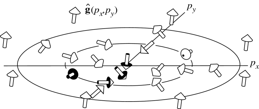
Figure 12: Skyrmion in ${\bf p}$-space with momentum space topological charge $\tilde{N}_{3}=-1$. It describes topologically non-trivial vacua in 2+1 systems with a fully non-singular Green’s function

An example is provided by the 2D version of the Hamiltonian (15) with $\hat{\bf l}=\hat{\bf z}$, $\hat{\bf e}_{1}=\hat{\bf x}$, $\hat{\bf e}_{2}=\hat{\bf y}$. Since for 2D case one has $p^{2}=p_{x}^{2}+p_{y}^{2}$, the quasiparticle energy (16)

$$E^{2}({\bf p})=\left({p_{x}^{2}+p_{y}^{2}\over 2m}-\mu\right)^{2}+\,c^{2}(p_{x}^{2}+p_{y}^{2})~{}$$ (44)

is nowhere zero except for $\mu=0$. The Hamiltonian (15) can be written in terms of the three-dimensional vector ${\bf g}(p_{x},p_{y})$:

$${\cal H}=\tau_{i}g_{i}({\bf p})~{}~{},~{}~{}g_{3}={p_{x}^{2}+p_{y}^{2}\over 2m}-\mu~{},~{}g_{1}=cp_{x}~{},~{}g_{2}=-cp_{y}~{}~{}.$$ (45)

For $\mu>0$ the distribution of the unit vector $\hat{\bf g}(p_{x},p_{y})={\bf g}/|{\bf g}|$ in the momentum space has the same structure as the skyrmion in real space (see Fig. 12). The topological invariant for this momentum-space skyrmion is given by Eq.(43) which can be rewritten in terms of the unit vector $\hat{\bf g}(p_{x},p_{y})$:

$$\tilde{N}_{3}={1\over 4\pi}\int dp_{x}dp_{y}~{}\hat{\bf g}\cdot\left({\partial\hat{\bf g}\over\partial{p_{x}}}\times{\partial\hat{\bf g}\over\partial{p_{y}}}\right)~{}.$$ (46)

Since at infinity the unit vector field $\hat{\bf g}$ has the same value, $\hat{\bf g}_{p\rightarrow\infty}\rightarrow(0,0,1)$, the 2-momentum space $(p_{x},p_{y})$ becomes isomoprhic to the compact $S^{2}$ sphere. The function $\hat{\bf g}({\bf p})$ realizes the mapping of this $S^{2}$ sphere to the $S^{2}$ sphere of the unit vector $\hat{\bf g}$ with winding number $\tilde{N}_{3}$. For $\mu>0$ one has $\tilde{N}_{3}=-1$ and for $\mu<0$ one has $\tilde{N}_{3}=0$.

5.2 Quantization of physical parameters

The topological charge $\tilde{N}_{3}$ and other similar topological charges in 2+1 systems give rise to quantization parameters. In particular, they are responsible for quantization of Hall and spin-Hall conductivities, which occurs without applied magnetic field (the so-called intrinsic or anomalous quantum Hall and spin quantum Hall effects). There are actually 4 responses of currents to transverse forces which are quantized under appropriate conditions. These are: (i) quantized response of the mass current (or electric current in electrically charged systems) to transverse gradient of chemical potential $\nabla\mu$ (transverse electric field ${\bf E}$); (ii) quantized response of the mass current (electric current) to transverse gradient of magnetic field interacting with Pauli spins; (iii) quantized response of the spin current to transverse gradient of magnetic field; and (iv) quantized response of the spin current to transverse gradient of chemical potential (transverse electric field) SQHE .

Chern-Simons term and ${\bf p}$-space topology

All these responses can be described using the generalized Chern-Simons term which mixes different gauge fields (see Eq.(21.20) in Ref. VolovikBook ):

$$F_{\rm CS}\{{\bf A}_{Y}\}={1\over 16\pi}N_{IJ}e_{\mu\nu\lambda}\int d^{2}xdtA_{\mu}^{I}F^{J}_{\nu\lambda}~{}~{}.$$ (47)

Here $A_{\mu}^{I}$ is the set of the real or auxiliary (fictituous) gauge fields. In electrically neutral systems, instead of the gauge field $A_{\mu}$ one introduces the auxiliary $U(1)$ field, so that the current is given by variation of the action with respect to $A_{\mu}$: $\delta S/\delta A_{\mu}=J^{\mu}$. The auxiliary $SU(2)$ gauge field $A_{\mu}^{i}$ is convenient for the description of the spin-Hall effect, since the variation of the action with respect to $A_{\mu}^{a}$ gives the spin current: $\delta S/\delta A_{\mu}^{i}=J^{\mu}_{i}$. Some components of the field $A_{\mu a}$ are physical, being represented by the real physical quantities which couple to the fermionic charges. Example is provided by the external magnetic field in neutral system, which play the role of $A_{0}^{i}$ (see Sec. 21.2 in Ref. VolovikBook ). After the current is calculated the values of the auxiliary fields are fixed. The latest discussion of the mixed Chern-Simons term can be found in Ref. MutualCS . For the related phenomenon of axial anomaly, the mixed action in terms of different (real and fictituous) gauge fields has been introduced in Ref. Zhitnitsky .

The important fact is that the matrix $N_{IJ}$ of the prefactors in the Chern-Simons action is expressed in terms of the momentum-space topological invariants:

$$N_{IJ}={1\over{24\pi^{2}}}e_{\mu\nu\lambda}~{}{\bf tr}~{}Q_{I}Q_{J}\int d^{2}pd\omega~{}G\partial_{p_{\mu}}G^{-1}G\partial_{p_{\nu}}G^{-1}G\partial_{p_{\lambda}}G^{-1}~{},$$ (48)

where $Q_{I}$ is the fermionic charge interacting with the gauge field $A_{\mu}^{I}$ (in case of several fermionic species, $Q_{I}$ is a matrix in the space of species).

Intrinsic spin quantum Hall effect

To obtain, for example, the response of the spin current $j_{z}^{i}$ to the electric field $E_{i}$, one must consider two fermionic charges: the electric charge $Q_{1}=e$ interacting with $U(1)$ gauge field, and the spin along $z$ as another charge, $Q_{2}=s_{z}=\hbar\sigma_{z}/2$, which interacts with the fictituous $SU(2)$ field $A_{\mu}^{z}$. This gives the quantized spin current response to the electric field $j_{z}^{i}=e^{ij}\sigma_{\rm spin-Hall}E_{j}$, where $\sigma_{\rm spin-Hall}=(e\hbar/8\pi)N$ and $N$ is integer:

$$N={1\over{24\pi^{2}}}e_{\mu\nu\lambda}~{}{\bf tr}~{}\sigma_{z}\int d^{2}pd\omega~{}G\partial_{p_{\mu}}G^{-1}G\partial_{p_{\nu}}G^{-1}G\partial_{p_{\lambda}}G^{-1}~{}.$$ (49)

Quantization of the spin-Hall conductivity in the commensurate lattice of vortices can be found in Ref. Vafek .

The above consideration is applicable, when the momentum (or quasi-momentum in solids) is the well defined quantity, otherwise (for example, in the presence of impurities) one cannot construct the invariant in terms of the Green’s function $G({\bf p},\omega)$. However, it is not excluded that in some cases the perturbative introduction of impurities does not change the prefactor $N_{IJ}$ in the Chern-Simons term (47) and thus does not influence the quantization: this occurs if there is no spectral flow under the adiabatic introduction of impurities. In this case the quantization is determined by the reference system – the fully gapped system from which the considered system can be obtained by the continuous deformation without the spectral flow (analogous phenomenon for the angular momentum paradox in ³He-A was discussed in AngularMomentumPar ). The most recent review paper on the spin current can be found in Rashba .

Momentum space topology and Hall effect in 3D systems

The momentum space topology is also important for the Hall effect in some 3+1 systems. The contribution of Fermi points to the intrinsic Hall effect is discussed in the Appendix of Ref. SplittingPreprint . For metals with Fermi surfaces having the global topological charge $N_{3}$ (see Sec. 3.3) the anomalous Hall effect is caused by the Berry curvature on the Fermi surface Haldane . The magnitude of the Hall conductivity is related to the volume of the Fermi surface in a similar way as the number of particles and the volume of the Fermi surface are connected by the Luttinger theorem Haldane . Another “partner” of the Luttinger theorem emerges for the Hall effect in superconductors, where topology enters via the spectral flow of fermion zero modes in the cores of topological defects – Abrikosov vortices EffectBandStructure .

5.3 Quantum phase transitions

Plateau transitions

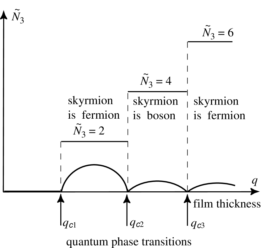
Figure 13: Quantum phase transitions occurring when one increases the thickness $q$ of the ³He-A film. The transitions at $q=q_{c2}$ and $q=q_{c3}$ are plateau-plateau transitions between vacua with different values of integer topological invariant $\tilde{N}_{3}$ in Eq.(43). At these transitions the quantum statistics of real-space skyrmions living in thin films changes. The change in the quasiparticle spectrum across the transitions may be seen from the minimum value of the quasiparticle energy, ${\rm min}_{\bf p}E({\bf p})$, at given $q$ (thick lines). The transitions at $q=q_{c2}$ and $q=q_{c3}$ between the fully gapped states occur through the gapless states. At $q=q_{c1}$ the transition is between gapless and fully gapped states

The integer topological invariant $\tilde{N}_{3}$ of the ground state cannot follow the continuous parameters of the system. That is why when one changes such a parameter, for example, the chemical potential in the model (45), one obtains the quantum phase transition at $\mu=0$ at which $\tilde{N}_{3}$ jumps from $0$ to $-1$. The film thickness is another relevant parameter. In the film with finite thickness the matrix of Green’s function acquires indices of the levels of transverse quantization. If one increases the thickness of the film, one finds a set of quantum phase transitions between vacua with different integer values of the invariant [Fig. 13], and thus between the plateaus in Hall or spin-Hall conductivity.

The abrupt change of the topological charge cannot occur adiabatically, that is why at the points of quantum transitions fermionic quasiparticles become gapless.

Topological zero modes and edge states

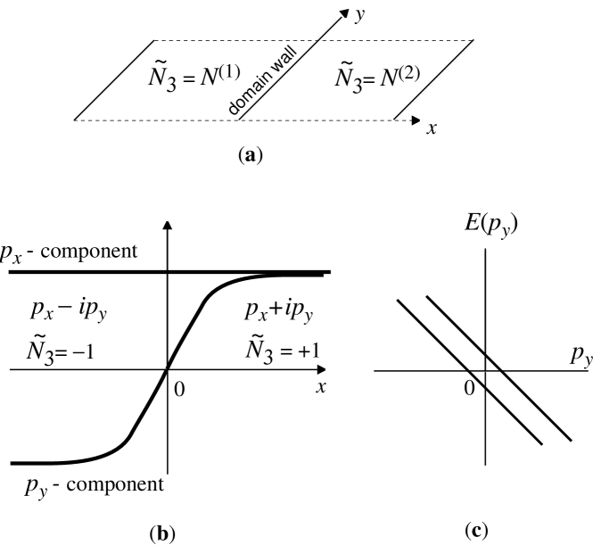
Figure 14: (a) Domain wall between two 2+1 vacua with different topological charges $\tilde{N}_{3}$. (b) Structure of the phase boundary between vacua with charges $\tilde{N}_{3}=\pm 1$ in Eq.(50). The prefactor in front of $p_{y}$ changes sign at $x=0$, which leads to the change of sign of the topological charge in Eq.(43). (c) Fermion zero modes – anomalous branches of fermions living at the interface whose spectrum crosses zero energy level. The number of anomalous branches is determined by the difference of the topological charges $\tilde{N}_{3}$ across the wall

If two vacua with different $\tilde{N}_{3}$ coexist in space [Fig. 14(a)], the phase boundary between them must also contain gapless fermions. This is an example of the so-called fermion zero modes living on different topological objects such as 3D monopole, 2D soliton wall, and 1D vortex/string (see Ref. JackiwRossi and references therein). The number of the gapless fermion zero modes obeys the index theorem: in our case the number of the $1+1$ fermions living at the phase boundary is determined by the difference of the topological charges of the two vacua, $\tilde{N}_{3}^{(1)}-\tilde{N}_{3}^{(2)}$ (see Chap. 22 in Ref. VolovikBook ).

The boundary of the condensed matter system can be considered as the phase boundary between the state with nonzero $\tilde{N}_{3}$ and the state with $\tilde{N}_{3}=0$. The corresponding fermion zero modes are the edge states well known in physics of the QHE.

Example of the phase boundary between two vacua with $\tilde{N}_{3}=\pm 1$ is shown in Fig. 14(b) for the $p_{x}+ip_{y}$ superfluids and superconductors. Here the $p_{y}$ component of the order parameter changes sign across the wall. The simplest structure of such boundary is given by Hamiltonian

$$H=\left(\matrix{\frac{p^{2}}{2m}-\mu&c\left(p_{x}+ip_{y}\tanh\frac{x}{\xi}\right)\cr c\left(p_{x}-ip_{y}\tanh\frac{x}{\xi}\right)&-\frac{p^{2}}{2m}+\mu\cr}\right)~{}.$$ (50)

Let us first consider fermions in semiclassical approach, when the coordinates $x$ and $p_{x}$ are independent. At $x=0$ the time reversal symmetry is restored, and the spectrum becomes gapless. At $x=0$ there are two zeroes of co-dimension 2 at points $p_{x}=0$ and $p_{y}=\pm p_{F}$. They are similar to zeroes discussed in Sec. 4.2. These zeroes are marginal, and disappear at $x\neq 0$ where the time reversal symmetry is violated. The topological charge is well defined only at $x\neq 0$. When $x$ crosses zero, the topological charge in Eq.(43) changes sign.

In the quantum mechanical description, $x$ and $p_{x}$ do not commute. The quantum-mechanical spectrum $E(p_{y})$ contains fermion zero modes – branches of spectrum which cross zero. According to the index theorem there are two anomalous branches in Fig. 14(c).

The index theorem together with the connection between the topological charge and quantization of physical parameters discussed in Sec. 5.2 implies that the quantization of Hall and/or spin Hall conductance is determined by the number of edge states in accordance with Refs. WenStone . The detailed discussion of the edge modes in $p_{x}+ip_{y}$ superfluids and superconductors and their contribution to the effective action can be found in Ref. Stonepxpy . These edge modes are Majorana fermions. Recent discussion of the edge states and intrinsic quantum spin-Hall effect in graphene is in Ref. Sengupta .

“Higgs” transition in ${\bf p}$-space

Note that the energy spectrum in Eq.(44) experiences an analog of the Higgs phase transition at $\mu=mc^{2}$ [Fig. 15]: if $\mu<mc^{2}$ the quasiparticle energy has a single minimum at $p=0$, while at $\mu>mc^{2}$ the minimum is at the circumference with radius $p_{0}=\sqrt{2m(\mu-mc^{2})}$. There is no symmetry breaking at this transition, since the vacuum state has the same rotational symmetry above and below the transition, while the asymptotic behavior of the thermodynamic quantities ($\propto T^{n}\exp{(-E_{\rm min}/T})$) experiences discontinuity across the transition: the power $n$ changes. That is why the point $\mu=mc^{2}$ marks the quantum phase transition, at which the topology of the minima of the energy spectrum changes.

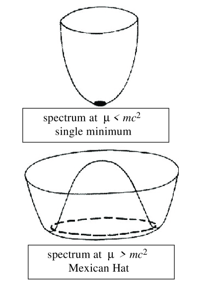
Figure 15: “Higgs” transition in momentum space.

However, this transition does not belong to the class of transitions which we discuss in the present review, since the topological invariant of the ground state $\tilde{N}_{3}$ does not change across this transition and thus at the transition point $\mu=mc^{2}$ the spectrum remains fully gapped. Moreover, such a transition does not depend on dimension of space-time and occurs in 3+1 systems as well. Example is provided by the $s$-wave superconductor or $s$-wave Fermi superfluid, whose spectrum in Eq.(5) experiences the same Higgs-like transition at $\mu=0$, i.e. in the BSC–BEC crossover region.

5.4 Quantum phase transition in 1D quantum Ising model

The momentum-space topology is applicable not only to fermionic systems, but to any system which can be expressed in terms of auxiliary fermions.

Fermionization and topological invariant

Example is provided by the 1-dimensional quantum Ising model where the topological quantum phase transition between the fully gapped vacua can be described in terms of the invariants for the fermionic Green’s function. The original Hamiltonian of this 1D chain of spins is:

$$H=-J\sum_{n=1}^{N}\left(h\sigma_{n}^{x}+\sigma_{n}^{z}\sigma_{n+1}^{z}\right)~{}~{},$$ (51)

where $\sigma^{x}$ and $\sigma^{z}$ are Pauli matrices, and $h$ is the parameter describing the external magnetic field. After the standard Jordan-Wigner transformation this system can be represented in terms of the non-interacting fermions with the following Hamiltonian in the continuous $N\rightarrow\infty$ limit (see Ref. Dziarmaga and references therein):

$$H=2J\left(h-\cos(pa)\right)\tau_{3}+2J\sin(pa)\tau_{1}~{}~{},~{}~{}-\frac{\pi}{a}<p<\frac{\pi}{a}~{}~{}.$$ (52)

It is periodic in the one-dimensional momentum space $p$ with period $2\pi/a$ where $a$ is the lattice spacing. The integer valued topological invariant here is the same as in Eq. (39) but now the integration is along the closed path in $p$-space, i.e. from $0$ to $2\pi/a$:

$$\tilde{N}_{2}=-{1\over 4\pi i}~{}{\rm tr}~{}\oint dp~{}\tau_{2}H^{-1}\nabla_{p}H~{}.$$ (53)

This invariant can be represented in terms of the Green’s function

$$G^{-1}=ig_{z}-g_{x}\tau_{3}+g_{y}\tau_{1}~{},$$ (54)

where for the particular case of the model (52), the components of the 3D vector ${\bf g}(p,\omega)$ are:

$$g_{x}(p,\omega)=2J\left(h-\cos(pa)\right)~{}~{},~{}~{}g_{y}(p,\omega)=2J\sin(pa)~{}~{},~{}~{}g_{z}(p,\omega)=\omega~{}.$$ (55)

Then the invariant (53) becomes:

$$\tilde{N}_{2}={1\over 4\pi}\int_{-\pi/a}^{\pi/a}dp\int_{-\infty}^{\infty}d\omega~{}\hat{\bf g}\cdot\left({\partial\hat{\bf g}\over\partial{p}}\times{\partial\hat{\bf g}\over\partial{\omega}}\right)~{}.$$ (56)

The invariant is well defined for the fully gapped states, when ${\bf g}\neq 0$ and thus the unit vector $\hat{\bf g}={\bf g}/|{\bf g}|$ has no singularity. In the model under discussion, one has for $h\neq 1$:

$$\tilde{N}_{2}(h<1)=1~{}~{},~{}~{}\tilde{N}_{2}(h>1)=0~{}~{}.$$ (57)

Instanton in $(p,\omega)$-space

The state with $\tilde{N}_{2}=1$ is the “instanton” in the $(\omega,p)$-space, which is similar to the skyrmion in $(p_{x},p_{y})$-space in Fig. 12. The real space-time counterpart of such instanton can be found in Refs. Instanton . It describes the periodic phase slip process occurring in superfluid ³He-A InstantonExp . In the model, the topological structure of the instanton at $h<1$ can be easily revealed for $h=0$. Introducing “space-time” coordinates $t=p$ and $z=\omega/2J$ one obtains that the unit vector $\hat{\bf g}$ precesses sweeping the whole unit sphere during one period $\Delta t=2\pi/a$ [Fig. 16]:

$$\hat{\bf g}(z,t)=\hat{\bf z}\cos\theta(z)+\sin\theta(z)\left(\hat{\bf x}\cos(at)+\hat{\bf y}\sin(at)\right)~{}~{},~{}~{}\cot\theta(z)=z~{}.$$ (58)

This state can be referred to as ‘ferromagnetic’, since in terms of spins it is the quantum superposition of two ferromagnetic states with opposite magnetization.

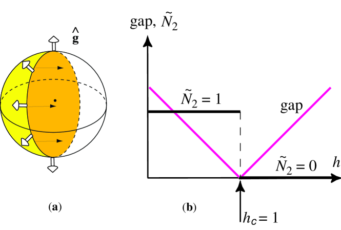
Figure 16: (a) Illustration of the topological invariant $\tilde{N}_{2}=1$ for ‘instanton’ in momentum space for $h=0$. According to Eq.(58) one has the domain wall in $z=\omega/2J$ space across which the direction of the vector ${\bf g}$ changes from $\hat{\bf z}$ at $z=\infty$ to $-\hat{\bf z}$ at at $z=-\infty$. The structure is periodic in $p$ and thus is precessing in ‘time’ $t=p$ (black arrows). During one period of precession $\Delta t=2\pi/a$ the unit vector $\hat{\bf g}(t,z)$ sweeps the whole unit sphere giving $\tilde{N}_{2}=1$ in Eq.(56). (b) At the transition point $h_{c}=1$ the gap in the energy spectrum of fermions vanishes, because the transition between two vacuua with different topological charge cannot occur adiabatically

At $h>1$, i.e. in the ‘paramagnetic’ phase, the momentum-space topology is trivial, $\tilde{N}_{2}(h>1)=0$. The transition at $h=1$ at which the topological charge $\tilde{N}_{2}$ of the ground state changes is the quantum phase transition, it only occurs at $T=0$.

Phase diagram for anisotropic XY-chain

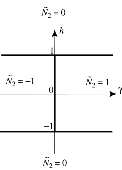
Figure 17: Phase diagram for anisotropic XY-chain in Eq.(59) in the plane ($\gamma,h)$. The regions with different topological charge $\tilde{N}_{2}$ are separated by the lines of topological quantum phase transitions (thick lines)

The phase diagram for the extension of the Ising model to the case of the anisotropic XY spin chain in a magnetic field with Hamiltonian (see e.g. Abanov )

$$H=-J\sum_{n=1}^{N}\left(h\sigma_{n}^{x}+\frac{1+\gamma}{2}\sigma_{n}^{z}\sigma_{n+1}^{z}+\frac{1-\gamma}{2}\sigma_{n}^{y}\sigma_{n+1}^{y}\right)~{}~{},$$ (59)

is shown in Fig. 17 in terms of the topological charge $\tilde{N}_{2}$. The lines $h=1$, $h=-1$ and ($\gamma=0$, $-1<h<1$), which separate regions with different $\tilde{N}_{2}$, are lines of quantum phase transitions.

Nullification of gap at quantum transition

Because of the jump in $\tilde{N}_{2}$ [Fig. 16(b)], the transition cannot occur adiabatically. That is why the energy gap must tend to zero at the transition, in the same way as it occurs at the plateau-plateau transition in Fig. 13. In the Ising model, the energy spectrum $E^{2}(p)=g_{x}^{2}(p)+g_{y}^{2}(p)=4J^{2}\left((h-\cos(pa))^{2}+\sin^{2}(pa)\right)$ has a gap $E(0)=2J|h-1|$ which tends to zero at $h\rightarrow 1$ [Fig. 16 (b)]. However, the nullification of the gap at the topological transition between the fully gapped states with different topological charges is the general property, which does not depend on the details of the underlying spin system and is robust to interaction between the auxiliary fermions.

The special case, when the gap does not vanish at the transition because the momentum space is not compact, is discussed in Sec. 11.4 of VolovikBook .

Dynamics of quantum phase transition and superposition of macroscopic states

In the quantum Ising model of Eq.(51) the ground state at $h<1$ represents the quantum superposition of two ferromagnetic states with opposite magnetization. However, in the limit of infinite number of spins $N\rightarrow\infty$ this becomes the Schrödinger’s Cat – the superposition of two macroscopically different states. According to Ref. Immirzi such superposition cannot be resolved by any measurements, because in the limit $N\rightarrow\infty$ no observable has matrix elements between the two ferromagnetic states, which are therefore disjoint. In general, the disjoint states form the equivalence classes emerging in the limit of infinite volume or infinite number of elements.

Another property of the disjoint macroscopic states is that their superposition, even if it is the ground state of the Hamiltonian, can never be achieved. For example, let us try to obtain the superposition of the two ferromagnetic states at $h<1$ starting from the paramagnetic ground state at $h>1$ and slowly crossing the critical point $h=1$ of the quantum phase transition. The dynamics of the time-dependent quantum phase transition in this model has been discussed in Refs. Dziarmaga ; ZurekQuantum . It is characterized by the transition time $\tau_{Q}$ which shows how fast the transition point is crossed: $1/\tau_{Q}=\dot{h}|_{h=1}$ . One may expect that if the transition occurs adiabatically, i.e. in the limit $\tau_{Q}\rightarrow\infty$, the ground state at $h>1$ transforms to the ground state at $h<1$. However, in the limit $N\rightarrow\infty$ the adiabatic condition cannot be satisfied. If $\tau_{Q}\rightarrow\infty$ but $\tau_{Q}\ll N^{2}/J$, the transition becomes non-adiabatic and the level crossing occurs with probability 1. Instead of the ground state at $h<1$ one obtains the excited state, which represents two (or several) ferromagnetic domains separated by the domain wall(s). Thus in the $N=\infty$ system instead of the quantum superposition of the two ferromagnetic states the classical coexistence of the two ferromagnetic states is realized.

In the obtained excited state the translational and time reversal symmetries are broken. This example of spontaneous symmetry breaking occurring at $T=0$ demonstrates the general phenomenon that in the limit of the infinite system one can never reach the superposition of macroscopically different states. On the connection between the process of spontaneous symmetry breaking and the measurement process in quantum mechanics see Ref. Grady and references therein. Both processes are emergent phenomena occurring in the limit of infinite volume $V$ of the whole system. In finite systems the quantum mechanics is reversible. For general discussion of the symmetry breaking phase transition in terms of the disjoint limit Gibbs distributions emerging at $V\rightarrow\infty$ see the book by Sinai Sinai .

6 Conclusion

Here we discussed the quantum phase transitions which occur between the vacuum states with the same symmetry above and below the transition. Such a transition is essentially different from conventional phase transition which is accompanied by the symmetry breaking. The discussed zero temperature phase transition is not the termination point of the line of the conventional 2-nd order phase transition: it is either an isolated point $(q_{c},0)$ in the $(q,T)$ plane, or the termination line of the 1-st order transition. This transition is purely topological – it is accompanied by the change of the topology of fermionic Green’s function in ${\bf p}$-space without change in the vacuum symmetry. The ${\bf p}$-space topology, in turn, depends on the symmetry of the system. The interplay between symmetry and topology leads to variety of vacuum states and thus to variety of emergent physical laws at low energy, and to variety of possible quantum phase transitions. The more interesting situations are expected for spatially inhomogeneous systems, say for systems with topological defects in ${\bf r}$-space, where the ${\bf p}$-space topology, the ${\bf r}$-space topology, and symmetry are combined (see Refs. Grinevich ; Horava and Chapter 23 in VolovikBook ).

I thank Frans Klinkhamer for collaboration and Petr Horava for discussions. This work is supported in part by the Russian Ministry of Education and Science, through the Leading Scientific School grant $\#$1157.2006.2, and by the European Science Foundation COSLAB Program.

References

- (1) H. Georgi, S.L. Glashow: Phys. Rev. Lett. 32, 438 (1974)
- (2) H. Georgi, H.R. Quinn, S. Weinberg: Phys. Rev. Lett. 33, 451 (1974)
- (3) G.E. Volovik, L.P. Gorkov: Sov. Phys. JETP 61, 843 (1985)
- (4) D. Vollhardt, P. Wölfle: The Superfluid Phases of Helium 3 (Taylor and Francis, London, 1990)
- (5) N.D. Mermin: Rev. Mod. Phys. 51, 591 (1979)
- (6) G.E. Volovik: The Universe in a Helium Droplet (Clarendon Press, Oxford, 2003)
- (7) P. Horava: Phys. Rev. Lett. 95, 016405 (2005)
- (8) V.A. Khodel, V.R. Shaginyan: JETP Lett. 51, 553 (1990)
- (9) G.E. Volovik: JETP Lett. 53, 222 (1991)
- (10) V.R. Shaginyan, A.Z. Msezane, M.Ya. Amusia: Phys. Lett. A 338, 393 (2005)
- (11) V.A. Khodel, J.W. Clark, M.V. Zverev: ‘Thermodynamic properties of Fermi systems with flat single-particle spectra’ (cond-mat/0502292)
- (12) V.A. Khodel, M.V. Zverev, V.M. Yakovenko: Phys. Rev. Lett. 95, 236402 (2005)
- (13) G.E. Volovik: JETP Lett. 59, 830 (1994)
- (14) S. Sachdev: Quantum Phase Transitions (Cambridge University Press, Cambridge, 2003)
- (15) I.M. Lifshitz: Sov. Phys. JETP 11, 1130 (1960); I.M. Lifshitz, M.Y. Azbel, M.I. Kaganov: Electron Theory of Metals (Consultant Press, New York, 1972)
- (16) G.E. Volovik: Exotic Properties of Superfluid 3He (World Scientific, Singapore, 1992)
- (17) F.R. Klinkhamer, G.E. Volovik: JETP Lett. 80, 343 (2004)
- (18) F.R. Klinkhamer, G.E. Volovik: Int. J. Mod. Phys. A 20, 2795 (2005)
- (19) V. Gurarie, L. Radzihovsky, A. V. Andreev: Phys. Rev. Lett. 94, 230403 (2005)
- (20) S.S. Botelho, C.A.R. Sa de Melo: J. Low Temp. Phys. 140, 409 (2005)
- (21) S.S. Botelho, C.A.R. Sa de Melo: Phys. Rev. B 71, 134507 (2005)
- (22) L.S. Borkowski, C.A.R. Sa de Melo: ‘From BCS to BEC superconductivity: Spectroscopic consequences’ (cond-mat/9810370)
- (23) R.D. Duncan, C.A.R. Sa de Melo: Phys. Rev. B 62, 9675 (2000)
- (24) X.G. Wen, A. Zee: Phys. Rev. B 66, 235110 (2002)
- (25) E. Gubankova: ‘Conditions for existence of neutral strange quark matter’ (hep-ph/0507291) E. Gubankova, E. Mishchenko, F. Wilczek: Phys. Rev. Lett. 94, 110402 (2005) K. Rajagopal, A. Schmitt: ‘Stressed pairing in conventional color superconductors is unavoidable’ (hep-ph/0512043) R. Casalbuoni: ‘Color Superconductivity in High Density QCD’ (hep-ph/0512198)
- (26) N. Bergeal, J. Lesueur, M. Aprili, G. Faini, J. P. Contour, B. Leridon: ‘Direct test of pairing fluctuations in the pseudogap phase of underdoped cuprates’ (cond-mat/0601265)
- (27) M.V. Sadovskii: ‘Models of the pseudogap state in high temperature superconductors’ (cond-mat/0408489)
- (28) E.Z. Kuchinskii, M.V. Sadovskii: ‘Non - Fermi liquid behavior in fluctuating gap model: From pole to zero of the Green’s function’ (cond-mat/0602406)
- (29) I. Dzyaloshinskii: Phys. Rev. Phys. Rev. B 68, 085113 (2003)
- (30) T.D. Stanescu, P.W. Phillips, T.P. Choy: cond-mat/0602280
- (31) T. Holstein, R.E. Norton, P. Pincus: Phys. Rev. B 8, 2649 (1973)
- (32) M.Yu. Reizer: Phys. Rev. B 40, 11571 (1989) M.Yu. Reizer: Phys. Rev. B 44, 5476 (1991) W.E. Brown, J.T. Liu, H.C. Ren: Phys.Rev. D 62 054013 (2000)
- (33) A. Ipp, A. Gerhold, A. Rebhan: Phys. Rev. D 69, 011901(R) (2004) T. Schäfer, K. Schwenzer: Phys. Rev. D 70, 054007 (2004) T. Schäfer: ‘Fermionic Quasiparticles in QCD at High Baryon Density’ (hep-ph/0510044)
- (34) A.V. Chubukov, D.V. Khveshchenko: cond-mat/0604376
- (35) J. von Neumann, E. Wigner: Phys. Zeit. 30, 467 (1929)
- (36) A.J. Stone: Proc. R. Soc. London A 351, 141 (1976)
- (37) V.I. Arnold: Mathematical Method in Classical Mechanics (Nauka, Moscow, 1979, in Russian) (Springer-Verlag, 1989)
- (38) M.V. Berry: Proc. R. Soc. London A 392, 45 (1984)
- (39) S.P. Novikov: Sov. Phys. Math. Dokl. 23, 298 (1981)
- (40) G.E. Volovik: JETP Lett. 46, 98 (1987)
- (41) H.B. Nielsen, M. Ninomiya: Nucl. Phys. B 185, 20 (1981) Nucl. Phys. B 193, 173 (1981)
- (42) X.G. Wen: Phys. Rev. Lett. 88, 011602 (2002)
- (43) F.R. Klinkhamer: ‘Lorentz-noninvariant neutrino oscillations: model and predictions’ (hep-ph/0407200) F.R. Klinkhamer: Nucl. Phys. B (Proc. Suppl.) 149, 209 (2005)
- (44) K. Kajantie, M. Laine, K. Rummukainen, M. Shaposhnikov: Phys. Rev. Lett. 77, 2887 (1996)
- (45) S.L. Adler: ‘Anomalies to all orders’. In: Fifty Years of Yang-Mills Theory, ed. by G. ’t Hooft (World Scientific, 2006)
- (46) E.I. Blount: Phys. Rev. B 32, 2935 (1985)
- (47) H.J.H. Smilde, A.A. Golubov, Ariando, G. Rijnders, J.M. Dekkers, S. Harkema, D.H.A. Blank, H. Rogalla, H. Hilgenkamp, Phys. Rev. Lett. 95, 257001 (2005)
- (48) K.S. Novoselov, A.K. Geim, S.V. Morozov, D. Jiang, M.I. Katsnelson, I.V. Grigorieva, S.V. Dubonos, A.A. Firsov: Nature 438, 197 (2005)
- (49) S.G. Sharapov, V.P. Gusynin, H. Beck: Phys. Rev. B 69, 075104 (2004)
- (50) K. S. Novoselov, E. McCann, S. V. Morozov, V. I. Falko, M. I. Katsnelson, U. Zeitler, D. Jiang, F. Schedin, A. K. Geim: ‘Unconventional quantum Hall effect and Berry’s phase of in bilayer graphene’ (cond-mat/0602565)
- (51) E. McCann, V.I. Fal’ko: Phys. Rev. Lett. 96, 086805 (2006)
- (52) M. Sato: ‘Nodal structure of superconductors with time-reversal invariance and topological number’ (cond-mat/0602445)
- (53) A.A. Kordyuk, S.V. Borisenko, A.N. Yaresko, S.-L. Drechsler, H. Rosner, T.K. Kim, A. Koitzsch, K.A. Nenkov, M. Knupfer, J. Fink, R. Follath, H. Berger, B. Keimer, S. Ono, Yoichi Ando: Phys. Rev. B 70, 214525 (2004) S. V. Borisenko, A. A. Kordyuk, V. Zabolotnyy, J. Geck, D. Inosov, A. Koitzsch, J. Fink, M. Knupfer, B. Buechner, V. Hinkov, C. T. Lin, B. Keimer, T. Wolf, S. G. Chiuzbaian, L. Patthey, R. Follath: ‘Kinks, nodal bilayer splitting and interband scattering in YBCO’ (cond-mat/0511596)
- (54) T. Yamasaki, K. Yamazaki, A. Ino, M. Arita, H. Namatame, M. Taniguchi, A. Fujimori, Z.-X. Shen, M. Ishikado, S. Uchida: ‘Unmasking the nodal quasiparticle dynamics in cuprate superconductors using low-energy photoemission’ (cond-mat/0603006)
- (55) G.E. Volovik: JETP Lett. 73, 162 (2001)
- (56) F.R. Klinkhamer: ‘Possible new source of T and CP violation in neutrino oscillations’ (hep-ph/0601116)
- (57) M. Consoli: Phys. Rev. D 65, 105017 (2002) M. Consoli, E. Costanzo: Nuovo Cim. B 119, 393 (2004)
- (58) G.E. Volovik: JETP Lett. 58, 469 (1993)
- (59) H. Balci, R.L. Greene: Phys. Rev. Lett. 93, 067001 (2004)
- (60) W. Yu, B. Liang, R.L. Greene: Phys. Rev. B 72, 212512 (2005)
- (61) K. Ishikawa, T. Matsuyama: Z. Phys. C 33, 41 (1986) K. Ishikawa, T. Matsuyama: Nucl. Phys. B 280, 523 (1987)
- (62) G.E. Volovik, V.M. Yakovenko: J. Phys.: Condens. Matter 1, 5263 (1989)
- (63) G.E. Volovik: ‘Fractional statistics and analogs of quantum Hall effect in superfluid 3He films’. In: Quantum Fluids and Solids - 1989 ed. by G.G.Ihas, Y.Takano (AIP Conference Proceedings , 1989) 194, pp. 136–146
- (64) Su-Peng Kou, Xiao-Liang Qi, Zheng-Yu Weng: Phys. Rev. B 72, 165114 (2005)
- (65) D.T. Son, A.R. Zhitnitsky: Phys. Rev. D 70, 074018 (2004)
- (66) O. Vafek and A. Melikyan: ‘Index theorem and quantum order of -wave superconductors in the vortex state’ (cond-mat/0509258)
- (67) G.E. Volovik: JETP Lett. 61, 958 (1995)
- (68) E.I. Rashba: ‘Spin-orbit coupling and spin transport’ (cond-mat/0507007) H.A. Engel, E.I. Rashba, B.I. Halperin: ‘Theory of Spin Hall Effects’ (cond-mat/0603306)
- (69) S.D.M. Haldane: Phys. Rev. Lett. 93, 206602 (2004)
- (70) G.E. Volovik: JETP Lett. 64, 845 (1996)
- (71) R. Jackiw, P. Rossi: Nucl.Phys. B 190, 681, (1981)
- (72) M. Stone: Ann. Phys. 207, 38 (1991) X.G. Wen: Phys. Rev. B 43, 11025 (1991)
- (73) M. Stone, R. Roy: Phys. Rev. B 69, 184511 (2004)
- (74) K. Sengupta, R. Roy, M. Maiti: ‘Spin-Hall effect in triplet chiral superconductors and graphene’ (cond-mat/0604217)
- (75) J. Dziarmaga: Phys. Rev. Lett. 95 245701 (2005)
- (76) J.R. Hook, H.E. Hall: J. Phys. C 12, 783 (1979) G.E. Volovik: JETP Lett. 27, 573 (1978)
- (77) D.N. Paulson, M. Krusius, J.C. Wheatley: Phys. Rev. Lett. 36, 1322 (1976)
- (78) A.G. Abanov, F. Franchini: Phys. Lett. A 316, 342 (2003)
- (79) M. Fioroni, G. Immirzi: ’How and why the wave function collapses after a measurement’ (gr-qc/9411044)
- (80) W.H. Zurek, U. Dorner, P. Zoller: Phys. Rev. Lett. 95, 105701 (2005)
- (81) M. Grady: ‘Spontaneous symmetry breaking as the mechanism of quantum measurement’ (hep-th/9409049)
- (82) Ya.G. Sinai: Theory of Phase Transitions, International series in natural philosophy (Pergamon Press, 1983)
- (83) P.G. Grinevich, G.E. Volovik: J. Low Temp. Phys. 72, 371 (1988) M.M. Salomaa, G.E. Volovik: Phys. Rev. 37, 9298 (1988) M.M. Salomaa, G.E. Volovik: J. Low Temp. Phys. 74, 319 (1989)