Statistical mechanics and Vlasov equation allow for a simplified Hamiltonian description of Single-Pass Free Electron Laser saturated dynamics

Abstract

A reduced Hamiltonian formulation to reproduce the saturated regime of a Single Pass Free Electron Laser, around perfect tuning, is here discussed. Asymptotically, $N_{m}$ particles are found to organize in a dense cluster, that evolves as an individual massive unit. The remaining particles fill the surrounding uniform sea, spanning a finite portion of phase space, approximately delimited by the average momenta $\omega_{+}$ and $\omega_{-}$. These quantities enter the model as external parameters, which can be self-consistently determined within the proposed theoretical framework. To this aim, we make use of a statistical mechanics treatment of the Vlasov equation, that governs the initial amplification process. Simulations of the reduced dynamics are shown to successfully capture the oscillating regime observed within the original $N$-body picture.

I General background

Free-Electron Lasers (FELs) are coherent and tunable radiation sources, which differ from conventional lasers in using a relativistic electron beam as their lasing medium, hence the term free-electron.

The physical mechanism responsible for the light emission and amplification is the interaction between the relativistic electron beam, a magnetostatic periodic field generated in the undulator and an optical wave copropagating with the electrons. Due to the effect of the magnetic field, the electrons are forced to follow sinusoidal trajectories, thus emitting synchrotron radiation. This spontaneous emission is then amplified along the undulator until the laser effect is reached. Among different schemes, single-pass high-gain FELs are currently attracting growing interest, as they are promising sources of powerful and coherent light in the UV and X ranges. Besides the Self Amplified Spontaneous Emission (SASE) setting sase , seeding schemes may be adopted where a small laser signal is injected at the entrance of the undulator and guides the subsequent amplification process seed . In the following we shall refer to the latter case. Basic features of the system dynamics are successfully captured by a simple one-dimensional Hamiltonian model introduced by Bonifacio and collaborators in Bonifacio . Remarkably, this simplified formulation applies to other physical systems, provided a formal translation of the variables involved is performed. As an example, focus on kinetic plasma turbulence, e.g.  the electron beam-plasma instability. When a weak electron beam is injected into a thermal plasma, electrostatic modes at the plasma frequency (Langmuir modes) are destabilized. The interaction of the Langmuir waves and the electrons constituting the beam can be studied in the framework of a self-consistent Hamiltonian picture ElskensBook , formally equivalent to the one in Bonifacio . In a recent paper andrea we established a bridge between these two areas of investigation (FEL and plasma), and exploited the connection to derive a reduced Hamiltonian model to characterize the saturated dynamics of the laser. According to this scenario, $N_{m}$ particles are trapped in the resonance, i.e. experience a bouncing motion in one of the (periodically repeated) potential wells, and form a clump that evolves as a single macro-particle localized in space. The remaining particles populate the surrounding halo, being almost uniformly distributed in phase space between two sharp boundaries, whose average momentum is labeled $\omega_{+}$ and $\omega_{-}$. The issue of providing a self-consistent estimate for the external parameters $N_{m}$, $\omega_{+}$ and $\omega_{-}$ is addressed and solved in this paper.

This long-standing problem was first pointed out by Tennyson et al. in the pioneering work tennyson and recently revisited in ElskensBook . A first attempt to calculate $N_{m}$ is made in tesi where a semi-analytical argument is proposed. In this respect, the strategy here proposed applies to a large class of phenomena whose dynamics can be modeled within a Hamiltonian framework ElskensBook ; Ruffo displaying the emergence of collective behaviour Kaneko .

The paper is organized as follows. In Section II we introduce the one-dimensional model of a FEL amplifier Bonifacio and review the derivation of the reduced Hamiltonian tennyson ; andrea . Section III recalls the statistical mechanics approach to estimate the saturated laser regime. In Sections IV to VI the analytic characterization of $N_{m}$, $\omega_{+}$ and $\omega_{-}$ is given in details and the results are then tested numerically in section VII. Finally, in Section VIII we sum up and draw our conclusions.

II From the self-consistent $N$-body Hamiltonian to the reduced formulation

Under the hypothesis of one-dimensional motion and monochromatic radiation, the steady state dynamics of a Single-Pass Free Electron Laser is described by the following set of equations:

$$\frac{{\mathrm{d}}\theta_{j}}{{\mathrm{d}}\bar{z}} = p_{j}\quad,$$ (1)

$$\frac{{\mathrm{d}}p_{j}}{{\mathrm{d}}\bar{z}} = -Ae^{i\theta_{j}}-A^{\ast}e^{-i\theta_{j}}\quad,$$ (2)

$$\frac{{\mathrm{d}}A}{{\mathrm{d}}\bar{z}} = i\delta A+\frac{1}{N}\sum_{j}e^{-i\theta_{j}}~{}\quad,$$ (3)

where $\bar{z}=2k_{w}\rho z\gamma_{r}^{2}/\langle\gamma\rangle_{0}^{2}$ is the rescaled longitudinal coordinate, which plays the role of time. Here, $\rho=[a_{w}\omega_{p}/(4ck_{w})]^{2/3}/\gamma_{r}$ is the so-called Pierce parameter, $\langle\gamma\rangle_{0}$ the mean energy of the electrons at the undulator’s entrance, $k_{w}=2\pi/\lambda_{w}$ the wave number of the undulator, $\omega_{p}=(4\pi e^{2}n/m)^{1/2}$ the plasma frequency, $c$ the speed of light, $n$ the total electron number density, $e$ and $m$ respectively the charge and mass of one electron. Further, $a_{w}=eB_{w}/(k_{w}mc^{2})$, where $B_{w}$ is the rms peak undulator field. Here $\gamma_{r}=\left(\lambda_{w}(1+a_{w}^{2})/2\lambda\right)^{1/2}$ is the resonant energy, $\lambda_{w}$ and $\lambda$ being respectively the period of the undulator and the wavelength of the radiation field. Introducing the wavenumber $k$ of the FEL radiation, the two canonically conjugated variables are ($\theta$,$p$), defined as $\theta=(k+k_{w})z-2\delta\rho k_{w}z\gamma_{r}^{2}/\langle\gamma\rangle_{0}^{2}$ and $p=(\gamma-\langle\gamma\rangle_{0})/(\rho\langle\gamma\rangle_{0})$. $\theta$ corresponds to the phase of the electrons with respect to the ponderomotive wave. The complex amplitude $A=A_{x}+iA_{y}$ represents the scaled field, transversal to $z$. Finally, the detuning parameter is given by $\delta=(\langle\gamma\rangle_{0}^{2}-\gamma_{r}^{2})/(2\rho\gamma_{r}^{2})$, and measures the average relative deviation from the resonance condition.

The above system of equations ($N$ being the number of electrons) can be derived from the Hamiltonian

$$H=\sum_{j=1}^{N}\frac{p_{j}^{2}}{2}-\delta I+2\sqrt{\frac{I}{N}}\sum_{j=1}^{N}\sin(\theta_{j}-\varphi),$$ (4)

where the intensity $I$ and the phase $\varphi$ of the wave are given by $A=\sqrt{I/N}\exp(-i\varphi)$. Here the canonically conjugated variables are $(p_{j},\theta_{j})$ for $1\leq j\leq N$ and $(I,\varphi)$. Besides the “energy” $H$, the total momentum $P=\sum_{j}p_{j}+I$ is also conserved. By exploiting these conserved quantities, one can recast the FEL equations of motion in the following form for the set of $2N$ conjugate variables ($q_{j},p_{j}$) farina :

$$\dot{q_{j}} = p_{j}-\frac{1}{\sqrt{NI}}\sum_{l=1}^{N}\sin q_{l}+\delta~{},$$ (5)

$$\dot{p_{j}} = -2\sqrt{\frac{I}{N}}\cos q_{j},$$ (6)

where the dot denotes derivation with respect to $\bar{z}$, and $q_{j}=\theta_{j}-\varphi\ {\mathrm{mod}}(2\pi)$ is the phase of the $j^{th}$ electron in a proper reference frame. The fixed points of system (5)-(6) are determined by imposing $\dot{q_{j}}=\dot{p_{j}}=0$ and solving:

$$p_{j}-\frac{1}{\sqrt{NI}}\sum_{l=1}^{N}\sin q_{l}+\delta = 0~{},$$ (7)

$$2\sqrt{\frac{I}{N}}\cos q_{j} = 0.$$ (8)

An elliptical fixed point is found for $q_{i}=\bar{q}=3\pi/2$. The conjugate momentum solves $({\bar{p}}+\delta)\sqrt{P/N-{\bar{p}}}+1=0$ and therefore depends on $P/N$. We shall return on this issue in the following Sections.

For a monokinetic initial beam with velocity resonant with the wave, equations (1), (2) and (3) predict an exponential instability and a late oscillating saturation for the amplitude of the radiation field. Numerical simulations fully confirm this scenario as displayed in fig. 1. In the single particle ($q,p$) space, a dense core of particles is trapped by the wave and behaves like a large “macro-particle”, that evolves coherently in the resonance. The distances between these particles do not grow exponentially fast (as is the case for chaotic motion) but grow at most linearly with time (for particles trapped in the resonance with different adiabatic invariants, i.e.essentially different action in the single particle pendulum-like description). This linear-in-time departure of the particles appears in the differential rotation in fig. 2, while the remaining particles are almost uniformly distributed between two oscillating boundaries. Having observed the formation of such structures in the phase-space allowed to derive a simplified Hamiltonian model to characterize the asymptotic evolution of the laser tennyson ; andrea . This reduced formulation consists in only four degrees of freedom, namely the wave, the macro-particle and the two boundaries delimiting the portion of space occupied by the so-called chaotic sea, i.e. the uniform halo surrounding the inner core.

Figure 1: Evolution of the radiation intensity as follows from equations (1), (2) and (3). $N=10^{4}$ electrons are simulated, for an initial mono-energetic profile. Here $\delta=0$ and $I(0)\simeq 0$. Particles are initially uniformly distributed in space.

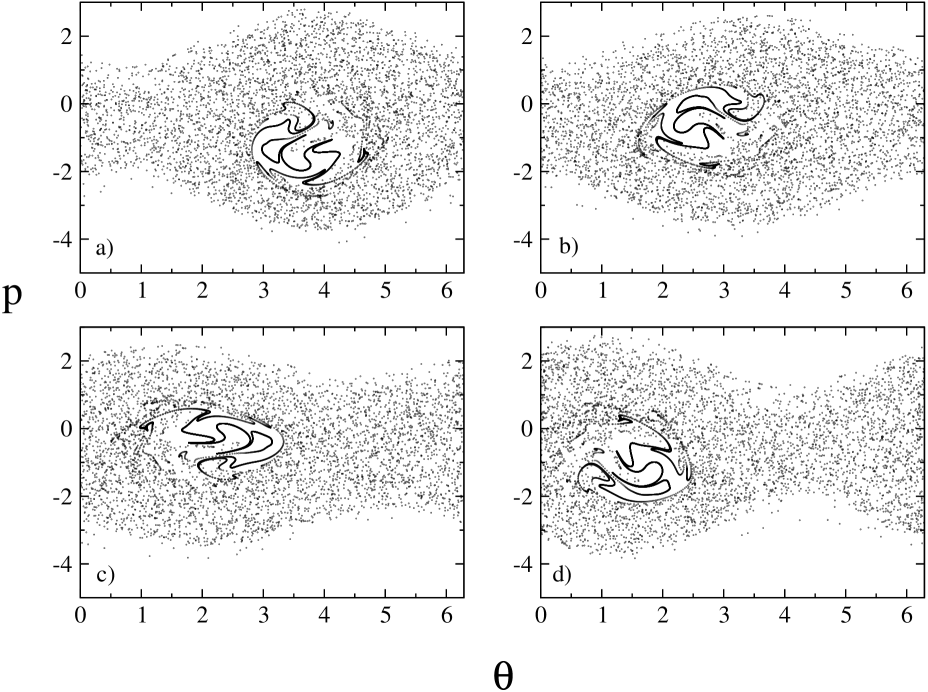
Figure 2: Phase space portraits for different position along the undulator [$\bar{z}$ = a) $80$, b) $81$, c) $83$, d) $84$]. The differential rotation of the macro-particle is clearly displayed. For the parameters choice refer to the caption of Fig. 1.

In andrea we hypothesized the macro-particle to be formed by $N_{m}$ individual massive units, and introduced the variables $(\zeta,\xi)$ to label its position in the phase space.

The $N_{c}=N-N_{m}$ particles of the surrounding halo are treated as a continuum with constant phase space distribution, $f_{sea}(\theta,p,\bar{z})=f_{c}$, between two boundaries, namely $p_{+}(\theta,\bar{z})$ and $p_{-}(\theta,\bar{z})$ such that:

$$p_{\pm}=p^{0}_{\pm}+\widetilde{p}_{\pm}\exp(i\theta)+\widetilde{p}_{\pm}^{*}\exp(-i\theta)~{},$$ (9)

where $p^{0}_{\pm}$ represents their mean velocity. These assumptions allow to map the original system, after linearizing with respect to $\widetilde{p}_{\pm}$, into andrea :

$$\ddot{\zeta} = i\Phi e^{i\zeta}-i\Phi^{\ast}e^{-i\zeta}$$ (10)

$$\frac{1}{2}\dot{V}_{\pm} = -\frac{i}{2}{\omega}_{\pm}V_{\pm}+i\Phi$$ (11)

$$\dot{\Phi} = \frac{i}{2}\frac{N_{c}}{N}\frac{V_{+}-V_{-}}{\omega_{+}-\omega_{-}}+i\frac{N_{m}}{N}e^{-i\zeta}+i\delta\Phi$$ (12)

where

$$A = -i\Phi$$ (13)

$$\widetilde{p}_{\pm} = V_{\pm}/2$$ (14)

$$\widetilde{p}^{0}_{\pm} = \omega_{\pm}$$ (15)

Normalizing the density in the chaotic sea to unity yields $f_{c}=1/(2\pi\Delta\omega)$, where $\Delta\omega:=\omega_{+}-\omega_{-}$ represents the (average) width of the chaotic sea. The above system can be cast in a Hamiltonian form by introducing new actions $I_{\pm}$ and their conjugate angles $\varphi_{\pm}$:

$$V_{+} = \sqrt{4\frac{I_{+}\Delta\omega}{N_{c}}}e^{-i\varphi_{+}}$$ (16)

$$V_{-} = \sqrt{4\frac{I_{-}\Delta\omega}{N_{c}}}e^{i\varphi_{-}}.$$ (17)

A pictorial representation of the main quantities involved in the analysis is displayed in fig. 3. In addition:

$$\Phi=iA=-\sqrt{\frac{I}{N}}e^{-i(\varphi+\frac{\pi}{2})}.$$ (18)

The reduced $4$-degrees-of-freedom Hamiltonian reads, up to a constant irrelevant to the evolution equations:

$$H_{4}=\frac{\xi^{2}}{2N_{m}}-\delta I+\omega_{+}I_{+}-\omega_{-}I_{-}-2\alpha\left[\sqrt{II_{+}}\sin(\varphi-\varphi_{+})-\sqrt{II_{-}}\sin(\varphi+\varphi_{-})\right]-2\beta\sqrt{I}\sin(\varphi-\zeta),$$ (19)

where

$$\alpha = \sqrt{\frac{N_{c}}{N\Delta\omega}}$$ (20)

$$\beta = \frac{N_{m}}{\sqrt{N}}$$ (21)

The first four terms represent the kinetic energy of the macro-particle, the oscillation of the wave and the harmonic contributions associated to the oscillation of the chaotic sea boundaries. The remaining terms refer to the interaction energy. Total momentum is $P=\xi+I+N_{c}\bar{\omega}$. The Hamiltonian (19) allows for a simplified description of the late nonlinear regime of the instability, provided the three parameters $\omega_{+}$, $\omega_{-}$ and $N_{m}$ are given.

To achieve a complete and satisfying theoretical description we need to provide an argument to self-consistently estimate these coefficients. To this end, we shall use the analytical characterization of the asymptotic behavior of the laser intensity and beam bunching (a measure of the electrons spatial modulation) obtained in julien with a statistical mechanics approach. In the next section these results are shortly reviewed.

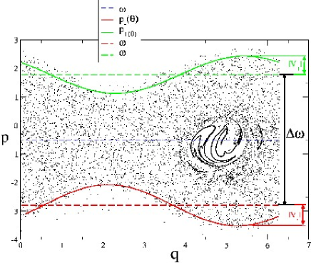
Figure 3: ($q$,$p$) phase space portrait in the deep saturated regime for a monokinetic initial beam ($I(0)\simeq 0$, $p_{j}(0)=0$ and $q$ uniformly distributed in $[0,2\pi]$). The two solid lines result from a numerical fit performed according to the following strategy. First, the particles located close to the outer boundaries are selected and then the expression $p_{\pm}(q)=\omega_{\pm}\mp|V_{\pm}|\sin(q+B_{\pm})$ is numerically adjusted to interpolate their distribution. Here, $|V_{\pm}|$, $B_{\pm}$ and $\omega_{\pm}$ are free parameters. The numerics are compatible with the simplifying assumption $B_{+}=B_{-}\simeq 0$.

III Statistical theory of Single-Pass FEL saturated regime

As observed in the previous Section, the process of wave amplification occurs in two steps: an initial exponential growth followed by a relaxation towards a quasi-stationary state characterized by large oscillations. This regime is governed by the Vlasov equation, rigorously obtained by performing the continuum limit ($N\rightarrow\infty$ at fixed volume and energy per particle) julien ; ElskensBook ; Firpo98 on the discrete system (1-3). Formally, the following Vlasov-wave system is found:

$$\frac{\partial f}{\partial\bar{z}} = -p\frac{\partial f}{\partial\theta}+2(A_{x}\cos{\theta}-A_{y}\sin{\theta})\frac{\partial f}{\partial p}\quad,$$ (22)

$$\frac{dA_{x}}{d\bar{z}} = -\delta A_{y}+\int f\cos{\theta}\,{\mathrm{d}}\theta\,{\mathrm{d}}p\quad,$$ (23)

$$\frac{dA_{y}}{d\bar{z}} = \delta A_{x}-\int f\sin{\theta}\,{\mathrm{d}}\theta\,{\mathrm{d}}p\quad.$$ (24)

The latter conserves the pseudo-energy per particle

$$\epsilon=\int{\frac{p^{2}}{2}f(\theta,p)\,{\mathrm{d}}\theta\,{\mathrm{d}}p}-\delta(A_{x}^{2}+A_{y}^{2})+2\int{(A_{x}\sin\theta+A_{y}\cos\theta)f(\theta,p)}\,{\mathrm{d}}\theta\,{\mathrm{d}}p$$ (25)

and the momentum per particle

$$\sigma=\int{pf(\theta,p)\,{\mathrm{d}}\theta\,{\mathrm{d}}p}+(A_{x}^{2}+A_{y}^{2})\ .$$ (26)

A subsequent slow relaxation towards the Boltzmann equilibrium is observed. This is a typical finite-$N$ effect and occurs on time-scales much longer than the transit trough the undulator ElskensBook ; Firpo01 ; Bonifacio . For our calculations we are interested in the first saturated state. To estimate analytically the average intensity and bunching parameter in this regime we exploit the statistical treatment of the Vlasov equation, presented in julien . In the following, we provide a short outline of the strategy. Since the Gibbs ensembles are equivalent for this model, note that the same expressions are recovered through a canonical calculation ElskensBook ; julien ; Firpo00 .

The basic idea is to coarse-grain the microscopic one-particle distribution function $f(\theta,p,\bar{z})$. An entropy is then associated to the coarse-grained distribution $\bar{f}$, which essentially counts a number of microscopic configurations. Neglecting the contribution of the field, since it represents only one degree of freedom within the ($N+1$) of the Hamiltonian (4), one assumes

$$s(\bar{f})=-\int{\left[\frac{\bar{f}}{f_{0}}\ln\frac{\bar{f}}{f_{0}}+\left(1-\frac{\bar{f}}{f_{0}}\right)\ln\left(1-\frac{\bar{f}}{f_{0}}\right)\right]f_{0}{\mathrm{d}}\theta\,{\mathrm{d}}p}\simeq-\int\left[\frac{\bar{f}}{f_{0}}\ln\frac{\bar{f}}{f_{0}}\right]f_{0}{\mathrm{d}}\theta{\mathrm{d}}p\ ,$$ (27)

where the constant $f_{0}$ is related to the initial distribution .

The equilibrium is computed by maximizing this entropy, while imposing the dynamical constraints. This corresponds to solving the constrained variational problem

$$S(\epsilon,\sigma)=\max_{\bar{f},A_{x},A_{y}}\left(s(\bar{f})\Big{|}H(\bar{f},A_{x},A_{y})=N\epsilon;P(\bar{f},A_{x},A_{y})=N\sigma;\int{f(\theta,p)\,{\mathrm{d}}\theta\,{\mathrm{d}}p}=1\right),$$ (28)

which leads to the equilibrium values

$$\bar{f} = f_{0}\frac{e^{-\beta(p^{2}/2+2A\sin\theta)-\lambda p-\mu}}{1+e^{-\beta(p^{2}/2+2A\sin\theta)-\lambda p-\mu}}$$ (29)

$$A = \sqrt{A_{x}^{2}+A_{y}^{2}}=\frac{\beta}{\beta\delta-\lambda}\int{\sin(\theta)\bar{f}(\theta,p)\,{\mathrm{d}}\theta\,{\mathrm{d}}p},$$ (30)

where $\beta$, $\lambda$ and $\mu$ are the Lagrange multipliers for the energy, momentum and normalization constraints and, in addition, we have assumed the non-restrictive condition $\sum\cos(\theta_{i})=0$ julien . Using then the three equations for the constraints, the statistical equilibrium calculation is reduced to finding the values of the multipliers as functions of energy $\epsilon$ and momentum $\sigma$. These equations lead directly to the estimates of the equilibrium values for the intensity $I$ and bunching parameter $b=|\sum\exp(i\theta_{i})|/N$.

In the following, we focus on the case of an initially monokinetic beam injected at the wave velocity, while the initial wave intensity is negligible, so that $\epsilon=0$ and $\sigma=0$. Moreover we let $f_{0}\rightarrow\infty$, which amounts to $\mu\rightarrow\infty$ in eq. (29). Results are displayed in fig. 4 showing remarkably good agreement between theory and simulations, below the critical threshold $\delta_{c}\simeq 1.9$ that marks the transition between high and low gain regimes. This transition is purely dynamical and cannot be reproduced by the statistical calculation.

Analytically, it turns out that

$$b=|A|^{3}-|A|\delta=\frac{{\mathrm{I}_{1}}(2/(3|A|^{3}-2\delta|A|))}{{\mathrm{I}_{0}}(2/(3|A|^{3}-2\delta|A|))}$$ (31)

where ${\mathrm{I}}_{n}$ is the modified Bessel function of order $n$. In particular for $\delta=0$, one finds $|A|^{2}=I/N\simeq 0.65$ and $b\simeq 0.54$.

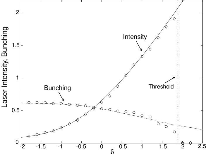
Figure 4: Comparison between theory (solid and long-dashed lines) and simulations (symbols) for a monoenergetic beam with $\epsilon=0$, $\sigma=0$, when varying the detuning $\delta$. The dotted vertical line, $\delta=\delta_{c}\simeq 1.9$, represents the transition from the high-gain to low gain regime Bonifacio .

IV Towards the analytical characterization of $N_{m}$

As previously discussed, one can predict the value of the bunching parameter $b$, using the above statistical mechanics description. Clearly, the bunching parameter $b$ depends on the spatial distribution of the particles. From its definition it immediately follows:

$$b=\left[\left(\frac{1}{N}\sum_{i=1}^{N}\cos q_{i}\right)^{2}+\left(\frac{1}{N}\sum_{i=1}^{N}\sin q_{i}\right)^{2}\right]^{1/2}.$$ (32)

To proceed we can isolate the contribution relative to the macroparticle from that associated to the chaotic sea. We thus obtain:

$$b=\left[\left(\frac{1}{N}\sum_{i\in macro}\cos q_{i}+\frac{1}{N}\sum_{i\in sea}\cos q_{i}\right)^{2}+\left(\frac{1}{N}\sum_{i\in macro}\sin q_{i}+\frac{1}{N}\sum_{i\in sea}\sin q_{i}\right)^{2}\right]^{1/2}.$$ (33)

Focus on the first two terms of expression (33). We assume the macroparticle to be ideally localized at the elliptic fixed point solving (7)-(8), i.e. set $q_{j}=\bar{q}=3\pi/2$, for each individual massive unit belonging to the inner agglomeration. Hence, $\sum_{i\in macro}\cos q_{i}=N_{m}\cos\bar{q}=0$. As concerns the second contribution, recalling the expressions for the boundaries $p_{-}(q)$ and $p_{+}(q)$ (see caption of fig. 3), one can formally write:

$$\frac{1}{N}\sum_{i\in sea}\cos q_{i} \simeq \frac{N_{c}}{N}\frac{1}{2\pi(\omega_{+}-\omega_{-})}\int_{0}^{2\pi}\cos q\int_{p_{-}(q)}^{p_{+}(q)}{\mathrm{d}}p{\mathrm{d}}q$$ (34)

$$= \frac{N_{c}}{N}\frac{1}{2\pi(\omega_{+}-\omega_{-})}\int_{0}^{2\pi}(\cos q)[\omega_{+}-\omega_{-}]{\mathrm{d}}q$$

$$-\frac{N_{c}}{N}\frac{1}{2\pi(\omega_{+}-\omega_{-})}\int_{0}^{2\pi}[(|V_{+}|+|V_{-}|)\sin q]\cos q{\mathrm{d}}q=0.$$

The other contributions in eq. (33) can be estimated as follows:

$$\frac{1}{N}\sum_{i\in macro}\sin q_{i}\simeq-\frac{N_{m}}{N}$$ (35)

while

$$\frac{1}{N}\sum_{i\in sea}\sin q_{i} \simeq \frac{N_{c}}{N}\frac{1}{2\pi(\omega_{+}-\omega_{-})}\int_{0}^{2\pi}(\sin q)\int_{p_{-}(q)}^{p_{+}(q)}{\mathrm{d}}p{\mathrm{d}}q$$ (36)

$$= \frac{N_{c}}{N}\frac{1}{2\pi(\omega_{+}-\omega_{-})}\underbrace{\int_{0}^{2\pi}\sin q(\omega_{+}-\omega_{-}){\mathrm{d}}q}_{=0}$$

$$-\frac{N_{c}}{N}\frac{1}{2\pi(\omega_{+}-\omega_{-})}\int_{0}^{2\pi}(|V_{+}|+|V_{-}|)\sin^{2}q{\mathrm{d}}q=-\frac{N_{c}}{N}\frac{\widetilde{V}}{2\Delta\omega},$$

where $\widetilde{V}=|V_{+}|+|V_{-}|$. Inserting (34), (35), (36) into (33) yields:

$$b=\frac{N_{m}}{N}+\frac{N_{c}}{N}\frac{\widetilde{V}}{2\Delta\omega}$$ (37)

and finally

$$\frac{N_{m}}{N}=\frac{2b\Delta\omega-\widetilde{V}}{2\Delta\omega-\widetilde{V}}=1-\frac{2(1-b)\Delta\omega}{2\Delta\omega-\widetilde{V}}$$ (38)

using the relation $N_{m}=N-N_{c}$. It is worth emphasizing that, neglecting as a first approximation the amplitudes of the sinusoidal boundaries, i.e. setting $V_{-}=V_{+}=0$, the previous equation reduces to

$$\frac{N_{m}}{N}=b~{},$$ (39)

confirming the relevance of the macroparticle picture to the bunching parameter, a physical quantity of paramount importance for the FEL dynamics. Formula (37) yields bunching parameter values larger than (39), i.e. implies that the sea also contributes to increasing the bunching parameter. The difference increases as the sea gets more populated and the width $\omega_{+}-\omega_{-}$ is reduced (note that our approximations require $|V_{+}|+|V_{-}|<\omega_{+}-\omega_{-}$, see fig. 3).

V Estimating the average momentum of the boundaries $\omega_{\pm}$

In this section we estimate the unknown quantities $\omega_{\pm}$ by characterizing their functional dependence on $N_{m}$. For this purpose we introduce (see schematic layout of fig. 3):

$$\omega_{\pm}=\bar{\omega}\pm\frac{\Delta\omega}{2}~{}.$$ (40)

The problem of estimating $\omega_{\pm}$ is obviously equivalent to providing a self-consistent calculation for $\bar{\omega}$ and $\Delta\omega$. The latter are both monitored as function of time in fig. 5 and shown to be practically constant.

In the following, we shall focus on the case of a system which evolved from an initially monokinetic beam and an initially infinitesimal wave. It is then convenient to choose the Galilean reference frame moving at the beam initial velocity. This translates into the conditions $\epsilon=0$ and $\sigma=0$. The detuning $\delta$ is arbitrary so far. It is of prime interest to consider the special case where the beam is injected at the resonant velocity, so that $\delta=0$. We shall make this additional assumption in section VII, but the estimates in this section and in the next one do not require it unless explicitly stated.

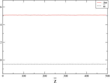
Figure 5: Solid line: $\Delta\omega$ vs $\bar{z}$. Dashed line: $\bar{\omega}$ vs $\bar{z}$. Parameters are set as discussed in the caption of fig. 1.

Consider the conservation of momentum for the original $N$-body system (4) and focus on the asymptotic dynamics, which allows one to isolate the contributions respectively associated to the macroparticle and the chaotic sea. Averaging over the number of particles yields:

$$\frac{N_{c}}{N}p_{sea}+\frac{N_{m}}{N}p_{macro}+J=\sigma_{0}$$ (41)

where $p_{sea}$ stands for the average momentum of the chaotic sea and the subscript ${}^{\prime}0^{\prime}$ labels the initial condition. To simplify the calculations, we introduced the rescaled intensity $J=I/N$. As already observed in andrea ; tennyson , the macroparticle rotates in phase space. This rotation is directly coupled to the oscillations displayed by the laser intensity. Averaging over a bounce period $z_{rot}$, one formally gets:

$$\frac{N_{c}}{N}\langle p_{sea}\rangle+\frac{N_{m}}{N}\langle p_{macro}\rangle+\langle J\rangle=0$$ (42)

where $\langle\cdot\rangle$ stands for the time average. Focus now on $\langle p_{sea}\rangle$. Since particles are uniformly filling the chaotic sea, one can use the approximation outlined before eq. (9) (see also caption of fig.3):

$$\langle p_{sea}\rangle=\frac{1}{z_{rot}}\int_{{\bar{z}}_{0}}^{{\bar{z}}_{0}+z_{rot}}\left(\int\!\!\int{pf_{sea}(\theta,p,\bar{z}){\mathrm{d}}\theta{\mathrm{d}}p}\right){\mathrm{d}}\bar{z}=\frac{1}{2\pi(\omega_{+}-\omega_{-})}\int\int_{p_{-}(q)}^{p_{+}(q)}{p}{\mathrm{d}}p{\mathrm{d}}\theta\simeq(\omega_{+}+\omega_{-})/2=\bar{\omega}~{}.$$ (43)

As already outlined in the preceding discussion, we assume that the macroparticle oscillates around the fixed point and therefore each individual element constituting the macroparticle verifies the condition $\langle q_{j}\rangle=\bar{q}$. In addition, from equation (7):

$$\langle p_{macro}\rangle:=\bar{p}=\left\langle\frac{1}{N\sqrt{J}}\sum_{i\in macro}\sin q_{i}\right\rangle+\left\langle\frac{1}{N\sqrt{J}}\sum_{i\in sea}\sin q_{i}\right\rangle-\delta.$$ (44)

To proceed in the analysis, we approximate the right hand side in equation (44) as:

$$\left\langle\frac{1}{N\sqrt{J}}\sum_{i\in macro}\sin q_{i}\right\rangle\simeq\frac{1}{N\sqrt{\langle J\rangle}}\sum_{i\in macro}\sin\langle q_{i}\rangle=\frac{1}{N\sqrt{\langle J\rangle}}\sum_{i\in macro}\sin\bar{q}=-\frac{N_{m}}{N}\frac{1}{\sqrt{\langle J\rangle}}$$ (45)

consistently with the argument after (33). The above relation is derived by performing a linearization (see Appendix), validated numerically and supported a posteriori by the correctness of the results. The contribution of the chaotic sea reads:

$$\left\langle\frac{1}{N\sqrt{J}}\sum_{i\in sea}\sin q_{i}\right\rangle\simeq\frac{1}{N\sqrt{\langle J\rangle}}\sum_{j\in sea}\sin q_{j}\simeq\frac{N_{c}}{N\sqrt{\langle J\rangle}}\frac{1}{2\pi(\Delta\omega)}\int_{0}^{2\pi}\sin q\int_{p_{-}(q)}^{p_{+}(q)}{\mathrm{d}}p{\mathrm{d}}q$$

$$=\frac{N_{c}}{N\sqrt{\langle J\rangle}}\frac{1}{2\pi\Delta\omega}\left[\underbrace{\int_{0}^{2\pi}(\omega_{+}-\omega_{-})\sin q{\mathrm{d}}q}_{=0}-\int_{0}^{2\pi}(|V_{+}|+|V_{-}|)\sin^{2}q{\mathrm{d}}q\right]=-\frac{N_{c}}{N\sqrt{\langle J\rangle}}\frac{\widetilde{V}}{2\Delta\omega}.$$ (46)

Merging equations (44), (45) and (V) and recalling (37) and (31), one obtains

$$\langle p_{macro}\rangle\simeq-\frac{N_{m}}{N}\frac{1}{\sqrt{\langle J\rangle}}-\frac{N_{c}}{N}\frac{\widetilde{V}}{2\Delta\omega}\frac{1}{\sqrt{\langle J\rangle}}-\delta=-\frac{b}{\sqrt{\langle J\rangle}}-\delta=-\langle J\rangle.$$ (47)

Thus the macroparticle moves on the average at the same velocity as the center of the chaotic sea. Inserting equations (43) and (47) into (42) and solving for $\bar{\omega}$, we find,

$$\bar{\omega}=\frac{N}{N_{c}}\left[-\langle J\rangle+\frac{N_{m}}{N}\left(\frac{b}{\sqrt{\langle J\rangle}}+\delta\right)\right]=-\langle J\rangle\ .$$ (48)

To get an expression for $\Delta\omega$, we consider the energy conservation for the original $N$-body model (4). By averaging over one complete rotation of the macroparticle, we write:

$$\frac{1}{N}\frac{\langle\sum_{i=1}^{N}p_{i}^{2}\rangle}{2}+2\left\langle\sqrt{J}\frac{1}{N}\sum_{i=1}^{N}\sin q_{i}\right\rangle=\delta\langle J\rangle~{}.$$ (49)

We then bring into evidence the contributions associated to the massive agglomerate and to the particles of the surrounding halo, for both the kinetic and the interaction terms:

$$\frac{N_{m}}{N}\frac{\langle p_{macro}^{2}\rangle}{2}+\frac{N_{c}}{N}\frac{\langle p_{sea}^{2}\rangle}{2}+\left\langle 2\sqrt{J}\frac{1}{N}\sum_{i\in macro}\sin q_{i}\right\rangle+\left\langle 2\sqrt{J}\frac{1}{N}\sum_{i\in sea}\sin q_{i}\right\rangle=\delta\langle J\rangle~{}.$$ (50)

Hereafter we make use of $\langle p_{macro}^{2}\rangle\simeq\langle p_{macro}\rangle^{2}$, which in turn amounts to assume small oscillations around the mean $\langle p_{macro}\rangle$, consistently with (44) which neglects such oscillations. The kinetic energy associated to the uniform sea can be estimated as follows:

$$\frac{\langle p_{sea}^{2}\rangle}{2}=\frac{1}{2\pi(\omega_{+}-\omega_{-})}\int{{\mathrm{d}}\theta\int_{\omega_{-}}^{\omega_{+}}{\frac{p^{2}}{2}}{\mathrm{d}}p}=\frac{1}{6}\frac{\omega_{+}^{3}-\omega_{-}^{3}}{\omega_{+}-\omega_{-}}=\frac{1}{6}\left(3\bar{\omega}^{2}+\frac{\Delta\omega^{2}}{4}\right).$$ (51)

In this estimate we assumed the particles to be distributed uniformly in a rectangular box, disregarding the sinusoidal shape of the boundaries. The modulation of the outer frontiers results in higher order corrections which can be neglected.

The interaction term follows directly from (44) and (47). Inserting (51) in (50), one finds:

$$\Delta\omega^{2}=\frac{N}{N_{c}}\left[36\langle J\rangle^{2}-24\delta\langle J\rangle\right].$$ (52)

VI Closed expressions for the amplitudes $V_{\pm}$ of the outer boundaries

The preceding calculations lead to three equations that allow to estimate $N_{m}$, $\bar{\omega}$ and $\Delta\omega$ (and thus $\omega_{+}$ and $\omega_{-}$), provided an expression for $V_{\pm}$ is given.

Note that $V_{\pm}$ enter as variables in the Hamiltonian and thus evolve self-consistently. However, one can assess their average value using an adiabatic argument ElskensBook . The boundaries of the sea are rather sharply drawn by the motion of particles, which move following the time-dependent Hamiltonian $H_{1.5}=p^{2}/2+2\sqrt{J}\sin(\theta-\varphi)$, with 1.5 degrees of freedom. In a first approximation, the time dependence of $J$ and $\varphi$ results in a detuning of the wave, as

$$\dot{\varphi}=\partial_{I}H=-\delta+(NI)^{-1/2}\sum_{j}\sin(\theta_{j}-\varphi)=-\delta-b/\sqrt{J}=-J$$ (53)

where we used (31) and the estimates of sec. IV. The resulting velocity agrees with the canonical estimate of reference ElskensBook in the low-temperature regime, as it must since ensembles are equivalent for this model.

Let us neglect the pulsations of $J$ and further variations of $\dot{\varphi}$. Then the Hamiltonian $H_{1.5}$ is brought to the integrable form of the classical pendulum, by a Galileo transformation to the frame moving at velocity $v=-\langle J\rangle$. In this frame, the motion of particles preserves their action, which is directly related to their effective energy

$$E_{\pm}=\frac{(p^{\prime}_{\pm})^{2}}{2}+2\sqrt{\langle J\rangle}\sin q^{\prime}$$ (54)

where $p^{\prime}_{\pm}=p_{\pm}+\langle J\rangle$, $q^{\prime}=\theta+\langle J\rangle t-\varphi^{\prime}$ ; here $\varphi^{\prime}=\varphi+\langle J\rangle t$ is the wave phase in the new frame. Solving for $p$, we get:

$$p_{\pm}+\langle J\rangle = \pm\sqrt{2E_{\pm}}\sqrt{1-\frac{2\sqrt{\langle J\rangle}}{E_{\pm}}\sin q^{\prime}}\simeq\pm\sqrt{2E_{\pm}}\left(1-\frac{\sqrt{\langle J\rangle}}{E_{\pm}}\sin q^{\prime}\right)$$ (55)

$$\simeq (\omega_{\pm}+\langle J\rangle)\mp|V_{\pm}|\sin q^{\prime}=\pm\left(\frac{\Delta\omega}{2}-|V_{\pm}|\sin q^{\prime}\right)$$

where we used the assumption that $\langle J\rangle^{1/2}/E_{\pm}$ is small, i.e. that the particle motion near the sea boundary (which has period $\sim 2\pi/\sqrt{2E_{\pm}}$) is fast with respect to the characteristic frequency $\sqrt{2}\langle J\rangle^{1/4}$ of particle oscillations inside the wave potential well. From (55) we finally obtain

$$|V_{\pm}|=\frac{4\sqrt{\langle J\rangle}}{\Delta\omega}~{}.$$ (56)

Note that the boundaries found here are also approximately level lines of the distribution $\bar{f}$ given by eq. (29), as they should be.

VII Validating the theory through direct simulation

In conclusion, we obtained a system of equations that can be solved to compute the values of $V_{+}$ and $V_{-}$ and provide self-consistent estimates of the three quantities $N_{m}$, $\omega_{+}$ and $\omega_{-}$, through a direct calculation of $\bar{\omega}$ and $\Delta\omega$, for an initially monokinetic beam and infinitesimal wave ($H/N=0$, $P/N=0$). The final equations read in the case $\delta=0$:

$$\frac{N_{m}}{N} = \frac{b-\widetilde{V}/(2\Delta\omega)}{1-\widetilde{V}/(2\Delta\omega)}$$

$$\bar{\omega} = -\langle J\rangle$$ (57)

$$\Delta\omega = 6\sqrt{\frac{N}{N_{c}}}\langle J\rangle$$

$$|V_{\pm}| = \frac{4\sqrt{\langle J\rangle}}{\Delta\omega}$$

$$\widetilde{V} = |V_{+}|+|V_{-}|$$

where $\langle J\rangle=|A|^{2}$ and $b$ are calculated from (31). The system is explicit after a few algebraic calculations, which show that

$${\frac{N_{c}}{N}}={9\over 2}b-\sqrt{{117\over 4}b^{2}-9b}\ .$$ (58)

It is worth recalling that the derivation of this system assumes that the dynamical variables like $V_{\pm}$ and $J$ do not vary too much, so that these final estimates yield coefficients $\omega_{\pm}$ which do not depend on time.

In table 1 the solutions of system (VII) are compared with the values measured in direct numerical experiments.

The theoretical values are then used to simulate the reduced dynamics (19). Comparisons with numerical results based on the original $N$-body (4) model are reported in fig. 6 and display a remarkably good agreement. The normalized standard deviations of the intensity in the two cases differ by less than five percent. As an additional check, we report in fig. 7 the Fourier transform of the signals displayed in fig. 6. A discrepancy smaller than $1$ % is observed for the peak values. These results provide an a posteriori validation of the reduced model which can be effectively employed to characterize the saturated evolution of the FEL field.

	Theory	Numerics
$b$	$0.530$	$0.56$
$\langle J\rangle$	$0.655$	$0.62$
$N_{m}/N$	$0.472$	$0.5$
$\bar{\omega}$	$-0.655$	$-0.50$
$\Delta\omega$	$5.408$	$5.10$
$|V_{+}|$	$0.599$	$0.85$
$|V_{-}|$	$0.599$	$0.8$

Table 1: Theoretical estimates from system (VII) (first column) vs. numerical measurements (second column) for $\delta=0$. To estimate $N_{m}$ we select the $i^{th}$ particle and calculate the spatial distances from the adjacent neighbors. If such quantities remain below a cut-off threshold during the subsequent evolution, the particles are said to belong to the inner cluster.

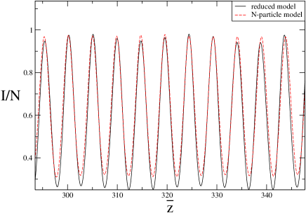
Figure 6: Rescaled laser intensity I/N vs time. The solid line refers to the reduced dynamics. The free parameters are fixed according to the self-consistent derivation here discussed. The dashed line refers to a direct integration of the original $N$-body system (4).

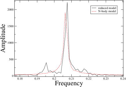
Figure 7: Fourier transform of the signals reported in fig. 6. The thick solid line refers to the reduced model, while the dashed one refers to the original $N$-body system.

VIII Conclusion

In this paper we consider a reduced Hamiltonian formulation to reproduce the saturated regime of a single-pass Free Electron Laser around perfect tuning. The model consists of only four degrees of freedom. The particles trapped in the resonance give birth to a coherent structure localized in space which is formally treated as an individual macro-particle. The remaining particles constitute the so-called chaotic sea and are uniformly distributed in phase space between two sharp boundaries that evolve according to the Vlasov equation.

This minimalistic approach was first derived by Tennyson et al. working in the context of plasma physics and recently adapted to the FEL in andrea . The original formulation assumes three external parameters, namely the mass of the dense core, $N_{m}$, and the average momenta $\omega_{\pm}$ associated to the outer boundaries, which have been so far phenomenologically adjusted to reproduce the results of $N$-body simulations. The lack of a self-consistent characterization has significantly weakened the potential impact of the reduced Hamiltonian approach so far.

This long standing problem tennyson ; ElskensBook is here addressed and solved. To this end we make use of the analytical estimates of the average intensity and bunching parameter at the saturation based on a statistical mechanics treatment of the Vlasov equation and of adiabatic theory ElskensBook ; julien . Our theoretical predictions for the parameters are compared to direct numerical measurements, showing an excellent agreement. Simulations of the reduced dynamics, complemented with the strategy here discussed, reproduce remarkably well the oscillatory regime displayed by the original $N$-body model.

In conclusion, we have provided a solid self-consistent formulation for the reduced Hamiltonian, which we hereby propose as an alternative theoretical tool to investigate the saturated regime of a FEL.

IX Acknowledgments

We thank R. Bachelard, C. Chandre and G. De Ninno for fruitful discussions. D.F. thanks Edison Giocattoli Firenze for financial support. Y.E. benefited from a delegation position at CNRS. This work is part of the PRIN2003 project Order and chaos in nonlinear extended systems funded by MIUR-Italy.

Appendix

Consider the following expression:

$$W=\frac{1}{N\sqrt{J}}\sum_{i\in macro}\sin q_{i}$$ (59)

and suppose we want to evaluate $\langle W\rangle$. The asymptotic intensity oscillates around a given plateau $\langle J\rangle$, hence we write the dominant Fourier term (see fig. 7):

$$J=\langle J\rangle\left(1+\epsilon_{J}\sin(\omega\bar{z})\right)$$ (60)

with $\epsilon_{J}=\Delta J/\langle J\rangle$, noting $\Delta J$ the amplitude of the oscillations. Moreover the macroparticle displays regular oscillations, centered around $\bar{q}=3\pi/2$. This in turn allows us to write:

$$q_{i}=\bar{q}+\epsilon_{q}\sin(\omega\bar{z})$$ (61)

for the $i^{th}$ particle composing the dense core. Here $\epsilon_{q}$ measures the average distance from $\bar{q}$. Assuming both $\epsilon_{J}$ and $\epsilon_{q}$ to be small, one can approximate (59) as follows:

$$W=\frac{N_{m}}{N\sqrt{\langle J\rangle}}\left(-1+\frac{\epsilon_{q}^{2}}{2}\sin^{2}(\omega\bar{z})+\ldots\right)\left(1-\frac{\epsilon_{J}}{2}\sin(\omega\bar{z})+\ldots\right)\simeq-\frac{N_{m}}{N\sqrt{\langle J\rangle}}+\frac{1}{2}\frac{N_{m}}{N\langle J\rangle^{1/2}}\epsilon_{J}\sin(\omega\bar{z})$$ (62)

where use has been made of the fact the $\cos{\bar{q}}=0$. Averaging (62) over one period $z_{rot}=2\pi/\omega$ one gets:

$$\langle W\rangle=-\frac{N_{m}}{N\sqrt{\langle J\rangle}}$$ (63)

which is identical to equation (45).