On the mean Euler characteristic and mean Betti’s numbers of the Ising model with arbitrary spin

Abstract

The behaviour of the mean Euler–Poincaré characteristic and mean Betti’s numbers in the Ising model with arbitrary spin on $\mathbbm{Z}^{2}$ as functions of the temperature is investigated through intensive Monte Carlo simulations. We also consider these quantities for each color $a$ in the state space $S_{Q}=\{-Q,-Q+2,\ldots,Q\}$ of the model. We find that these topological invariants show a sharp transition at the critical point.

Keywords: Phase transitions and critical phenomena. Topological invariants (Euler–Poincaré characteristic, Betti’s numbers).

1 Introduction

Knowledge about the spatial structure of systems is a subject that attracts more and more interest in statistical physics. For example, the study of morphological features has proved very useful to identify and distinguish various formation processes in contexts as varied as the study of large scale distributions of galaxies, or the investigation of micro-emulsions [1]. Other examples of situations where the focus on the spatial structure is of primary importance to understand the physical properties of a given system are provided by dissipative structures in hydrodynamics, Turing patterns occurring in chemical reactions, or transport properties of fluids [2]. For instance, the transport of a fluid over a porous substrate depends crucially on the existence of a connected cluster of pores that spans through the whole system [3]. Gaining insight into the spatial structure of the most commonly used lattice-models in statistical physics -i.e. the Potts, Clock and generalized Ising models- is also a matter of interest in the field of image-analysis, which makes extensive use of these models to simulate noise and clean dirty images [4]. In this context, mathematical quantities that characterize the typical spatial structure of the model seem to be the most natural tuning parameters as opposed to the usual thermodynamic quantities.
Consequently, efforts have recently been made [3, 5, 6] to study the typical behavior of Minkowsky-functionals (or curvature integrals) which quantify the geometrical properties of a given system. Particular interest has been devoted to the study of the Euler-Poincaré characteristic which turns out to be a relevant quantity in various models : let us indeed recall, that for the problem of bond percolation on regular lattices, Sykes and Essam [7] were able to show, using standard planarity arguments, that for the case of self-dual lattices (e.g. $\mathbb{Z}^{2}$), the mean value of the Euler-Poincaré characteristic changes sign at the critical point, see also [8].
More recently Blanchard, et al. showed [6] using duality and perturbative arguments, that for the two dimensional random cluster model (the Fortuin-Kasteleyn representation of the q-state Potts model) the mean local Euler-Poincaré characteristic is either zero or exhibits a jump at the self-dual temperature. More precisely, it vanishes when $q=1$ and exhibits a jump of order $1/\sqrt{q}$ when $q$ is large enough. Similar results were shown in higher dimensions $d$.
This paper aims to investigate the spatial structure of the Ising model with arbitrary spins on $\mathbb{Z}^{2}$ which, unlike the Potts-model, does not have a color-symmetry. We introduce colored complexes (i.e. the sets of sites for a given configuration that belong to the same color) and study the behavior of the associated local mean Euler-Poincaré characteristics. As a result of our numerical computations, we obtain that the mean value of the Euler characteristic per site vanishes below the critical temperature and is positive above this temperature. As we shall see, this behaviour can be related to the behaviours of topological invariants, the Betti’s numbers.

The paper is organized as follows. In Section 2, we introduce the model and give the definitions of the principal quantities of interest. Section 3 is devoted to the results obtained by intensive Monte-Carlo simulations. Concluding remarks are given in section $4$.

2 Definitions

To introduce the generalized Ising model considered by Griffiths’ in [9], we associate to each lattice site $x\in\mathbbm{Z}^{2}$ a spin $\sigma_{x}$ in the set $S_{Q}=\{-Q,-Q+2,\ldots,Q\}$, $Q=1,2,\ldots,$ (with cardinality $|S_{Q}|=Q+1$). The Hamiltonian in a finite box $\Lambda\subset\mathbbm{Z}^{2}$ is given by:

$$H_{\Lambda}=-J\sum_{\langle x,y\rangle}\sigma_{x}\sigma_{y}$$ (1)

where $J$ is a positive constant that we will take equal to $1$ in the next section, and the sum runs over nearest neighbors pairs of $\Lambda$. The associated partition function is defined by:

$$Z_{\Lambda}(\beta)=\sum_{{\begin{array}[]{c}\sigma_{x}\in S_{Q}\\ x\in\Lambda\end{array}}}e^{-\beta H_{\Lambda}}$$ (2)

where the sum is over all configurations $\boldsymbol{\sigma}_{\Lambda}=\{\sigma_{x}\}_{x\in\Lambda}$ and we let

$$\langle f\rangle_{\Lambda}(\beta)=\frac{1}{Z_{\Lambda}(\beta)}\sum_{{\begin{array}[]{c}\sigma_{x}\in S_{Q}\\ x\in\Lambda\end{array}}}fe^{-\beta H_{\Lambda}}$$ (3)

denote the (corresponding expectation) of a measurable function $f$. Among the quantity of interest, we shall first consider the magnetization

$$m_{\Lambda}(\beta)=\frac{1}{|\Lambda|}\langle\sum_{x\in\Lambda}\sigma_{x}\rangle_{\Lambda}(\beta)$$ (4)

where $|\Lambda|$ is the number of sites of $\Lambda$. Let us recall that this system exhibits a spontaneous magnetization at all inverse temperatures greater than the critical temperature of the Ising model ($Q=1$), as proved in [9].

We next introduce others quantities, namely the mean Euler characteristic per site. Consider a configuration $\boldsymbol{\sigma}_{\Lambda}$, and let $L(\boldsymbol{\sigma}_{\Lambda})$ be the set of bonds (unit segments) with endpoints $x,y$, such that $\sigma_{x}=\sigma_{y}$, and $P(\boldsymbol{\sigma}_{\Lambda})$ be the set of plaquettes $p$ with corner $x,y,z,t$, such that $\sigma_{x}=\sigma_{y}=\sigma_{z}=\sigma_{t}$. To a given configuration $\boldsymbol{\sigma}_{\Lambda}$, we associate (in a unique way) the two–dimensional cell–subcomplex $C(\boldsymbol{\sigma}_{\Lambda})=\{\Lambda,L(\boldsymbol{\sigma}_{\Lambda}),P(\boldsymbol{\sigma}_{\Lambda})\}$ of the complex $C=\{\Lambda,L_{\Lambda},P_{\Lambda}\}$ where $L_{\Lambda}$ is the set of bonds with both endpoints in $\Lambda$ and $P_{\Lambda}$ is the set of plaquettes with corners in $\Lambda$. The Euler characteristic of this subcomplex is defined by:

$$\boldsymbol{\chi}(\boldsymbol{\sigma}_{\Lambda})=|\Lambda|-|L(\boldsymbol{\sigma}_{\Lambda})|+|P(\boldsymbol{\sigma}_{\Lambda})|$$ (5)

where $|E|$ denotes hereafter the cardinality of the set $E$. It satisfies the Euler–Poincaré formula

$$\boldsymbol{\chi}(\boldsymbol{\sigma}_{\Lambda})=\boldsymbol{\pi}^{0}(\boldsymbol{\sigma}_{\Lambda})-\boldsymbol{\pi}^{1}(\boldsymbol{\sigma}_{\Lambda})+\boldsymbol{\pi}^{2}(\boldsymbol{\sigma}_{\Lambda})$$ (6)

where $\boldsymbol{\pi}^{0}(\boldsymbol{\sigma}_{\Lambda})$ and $\boldsymbol{\pi}^{1}(\boldsymbol{\sigma}_{\Lambda})$ are respectively the number of connected components and the number of independent $1$-cycles of the subcomplex $C(\boldsymbol{\sigma}_{\Lambda})$. Here $\boldsymbol{\pi}^{2}(\boldsymbol{\sigma}_{\Lambda})=0$ because $C(\boldsymbol{\sigma}_{\Lambda})$ has no $2$-cycles.

Notice that

$$\boldsymbol{\chi}(\sigma_{\Lambda})=\sum_{x\in\Lambda}\boldsymbol{\chi}_{x,\operatorname{loc}}(\boldsymbol{\sigma}_{\Lambda})$$ (7)

where the local Euler characteristic $\boldsymbol{\chi}_{x,\operatorname{loc}}(\boldsymbol{\sigma}_{\Lambda})$ is given by:

$$\boldsymbol{\chi}_{x,\operatorname{loc}}(\boldsymbol{\sigma}_{\Lambda})=1-\frac{1}{2}\sum_{y\in V(x)}\delta(\sigma_{x},\sigma_{y})+\frac{1}{4}\sum_{p\ni x}\prod_{yz\in p}\delta(\sigma_{y},\sigma_{z})$$ (8)

Here, $V(x)$ is the set of nearest neighbours of $x$, the second sums is over plaquettes containing $x$ as a corner, and $\delta$ is the kronecker symbol: $\text{}\delta(\sigma_{x},\sigma_{y})=1$ if $\sigma_{x}=\sigma_{y}$, and $\delta(\sigma_{x},\sigma_{y})=0$ otherwise. We define the mean Euler characteristic per site and the mean Betti’s numbers per site by:

$$\chi_{\Lambda}(\beta) = \frac{1}{|\Lambda|}\langle\boldsymbol{\chi}(\boldsymbol{\sigma}_{\Lambda})\rangle_{\Lambda}(\beta)\text{{{(1)}}}$$

$$\pi^{0}_{\Lambda}(\beta) = \frac{1}{|\Lambda|}\langle\boldsymbol{\pi}^{0}(\boldsymbol{\sigma}_{\Lambda})\rangle_{\Lambda}(\beta)\text{{{(2)}}}$$

$$\pi^{1}_{\Lambda}(\beta) = \frac{1}{|\Lambda|}\langle\boldsymbol{\pi}^{1}(\boldsymbol{\sigma}_{\Lambda})\rangle_{\Lambda}(\beta)\text{{{(3)}}}$$

The following limits exist and coincide:

$$\lim_{\Lambda\uparrow\mathbbm{Z}^{2}}\chi_{\Lambda}(\beta)=\lim_{\Lambda\rightarrow\mathbbm{Z}^{2}}\langle\boldsymbol{\chi}_{0,\operatorname{loc}}(\boldsymbol{\sigma}_{\Lambda})\rangle_{\Lambda}(\beta)$$ (9)

Here the first limit is taken in such a way that the number of sites of the boundary of $\Lambda$ divided by the number of sites of $\Lambda$ tends to $0$, while there is no restriction in the second limit.

The existence of these limits are simple consequences of Griffith’s inequality [10] which states that:

$$\langle\sigma_{x}^{n}\sigma_{y}^{m}\rangle_{\Lambda}(\beta)\geqslant\langle\sigma_{x}^{n}\rangle_{\Lambda}(\beta)\langle\sigma_{y}^{m}\rangle_{\Lambda}(\beta)$$ (10)

This implies the following monotonicity properties with respect to the volume:

$$\left\langle\sigma_{x}^{n}\sigma_{y}^{m}\rangle_{\Lambda}(\beta)\leqslant\left\langle\sigma_{x}^{n}\sigma_{y}^{m}\rangle_{\Lambda^{\prime}}(\beta)\operatorname{if}\Lambda\subset\Lambda^{\prime}\right.\right.$$

These properties give the existence of the infinite volume limit

$$\langle\sigma_{x}^{n}\sigma_{y}^{m}\rangle_{\Lambda}(\beta):={\lim_{\Lambda\rightarrow\mathbbm{Z}^{2}}}\langle\sigma_{x}^{n}\sigma_{y}^{m}\rangle_{\Lambda}(\beta)$$

through sequences of increasing volumes. They imply also, following [10], that the limiting state is translation invariant. It is then sufficient to observe that:

$$\delta(\sigma_{x},\sigma_{y})=\frac{\prod_{b\in S_{Q},b\neq 0}[b-(\sigma_{x}-\sigma_{y})]}{\prod_{b\in S_{Q},b\neq 0}b}$$

and thus can be written as a (finite) linear combination $\sum_{n,m\in S_{Q}}\lambda_{a,b}\sigma_{x}^{n}\sigma_{y}^{m}$ with finite coefficients $\lambda_{a,b}$ to conclude the existence of the second limit in (9), since also by (8) the local Euler characteristic is a (finite) linear combination of the $\sigma_{x}^{n}\sigma_{y}^{m}$ with finite coefficients. The translation invariance allows finally to show that this second limit in (9) coincides with the first one under the above mentioned conditions.

We shall also consider the subcomplexes of $C(\boldsymbol{\sigma}_{\Lambda})$ attached to each color. Namely, for a given configuration $\boldsymbol{\sigma}_{\Lambda}$ and a given color $a\in S_{Q}$, we let $\Lambda_{a}$ be the subset of the box $\Lambda$ such that $\sigma_{x}=a$, $L_{a}(\boldsymbol{\sigma}_{\Lambda})$ be the subset of bonds of $L(\boldsymbol{\sigma}_{\Lambda})$ with endpoints $x,y,$ such that $\sigma_{x}=\sigma_{y}=a$, and $P_{a}(\boldsymbol{\sigma}_{\Lambda})$ be the subset of plaquettes of $P(\boldsymbol{\sigma}_{\Lambda})$ with corner $x,y,z,t$, such that $\sigma_{x}=\sigma_{y}=\sigma_{z}=\sigma_{t}=a$. For each color $a$, we associate to a given configuration $\boldsymbol{\sigma}_{\Lambda}$, the two–dimensional cell–subcomplex $C_{a}(\boldsymbol{\sigma}_{\Lambda})=\{\Lambda_{a},L_{a}(\boldsymbol{\sigma}_{\Lambda}),P_{a}(\boldsymbol{\sigma}_{\Lambda})\}$. Obviously $C_{a}(\boldsymbol{\sigma}_{\Lambda})$ is a subcomplex of $C(\boldsymbol{\sigma}_{\Lambda})$ and hence a subcomplex of $C$ and $C(\boldsymbol{\sigma}_{\Lambda})=\cup_{a\in S_{Q}}\text{$C_{a}(\boldsymbol{\sigma}_{\Lambda})$}$.

The Euler characteristics of these subcomplexes are defined by:

$$\boldsymbol{\chi}^{a}(\boldsymbol{\sigma}_{\Lambda})=|\Lambda_{a}|-|L_{a}(\boldsymbol{\sigma}_{\Lambda})|+|P_{a}(\boldsymbol{\sigma}_{\Lambda})|$$ (11)

They satisfy the Euler–Poincaré formula

$$\boldsymbol{\chi}^{a}(\boldsymbol{\sigma}_{\Lambda})=\boldsymbol{\pi}^{0,a}(\boldsymbol{\sigma}_{\Lambda})-\boldsymbol{\pi}^{1,a}(\boldsymbol{\sigma}_{\Lambda})+\boldsymbol{\pi}^{2,a}(\boldsymbol{\sigma}_{\Lambda})$$ (12)

where $\boldsymbol{\pi}^{0,a}(\boldsymbol{\sigma}_{\Lambda})$ and $\boldsymbol{\pi}^{1,a}(\boldsymbol{\sigma}_{\Lambda})$ are respectively the number of connected components and the maximal number of independent $1$-cycles of the subcomplex $C_{a}(\boldsymbol{\sigma}_{\Lambda})$. Here again $\boldsymbol{\pi}^{2,a}(\boldsymbol{\sigma}_{\Lambda})=0$ because $C_{a}(\boldsymbol{\sigma}_{\Lambda})$ has no $2$-cycles.

Note that

$$\boldsymbol{\chi}(\boldsymbol{\sigma}_{\Lambda})=\sum_{a\in S_{Q}}\boldsymbol{\chi}^{a}(\boldsymbol{\sigma}_{\Lambda})$$ (13)

As for the total Euler characteristic, the Euler characteristic of each color can be written as a sum over local variables:

$$\boldsymbol{\chi}^{a}(\sigma_{\Lambda})=\sum_{x\in\Lambda}\boldsymbol{\chi}^{a}_{x,\operatorname{loc}}(\boldsymbol{\sigma}_{\Lambda})$$ (14)

where

$$\boldsymbol{\chi}^{a}_{x,\operatorname{loc}}(\boldsymbol{\sigma}_{\Lambda})=\delta(\sigma_{x},a)-\frac{1}{2}\sum_{y\in V(x)}\delta(\sigma_{x},a)\delta(\sigma_{y},a)+\frac{1}{4}\sum_{p\ni x}\prod_{yz\in p}\delta(\sigma_{y},a)\delta(\sigma_{z},a)$$ (15)

We define the mean Euler characteristic per site and the mean Betti’s numbers per site of the colored subcomplexes:

$$\chi^{a}_{\Lambda}(\beta) = \frac{1}{|\Lambda|}\langle\boldsymbol{\chi}^{a}(\sigma_{\Lambda})\rangle_{\Lambda}(\beta)\text{{{(4)}}}$$

$$\pi^{0,a}_{\Lambda}(\beta) = \frac{1}{|\Lambda|}\langle\text{$\boldsymbol{\pi}^{0,a}(\boldsymbol{\sigma}_{\Lambda})$}\rangle_{\Lambda}(\beta)\text{{{(5)}}}$$

$$\pi^{1,a}_{\Lambda}(\beta) = \frac{1}{|\Lambda|}\langle\text{$\boldsymbol{\pi}^{1,a}(\boldsymbol{\sigma}_{\Lambda})$}\rangle_{\Lambda}(\beta)\text{{{(6)}}}$$

One can show that the following limit exist and coincide:

$$\lim_{\Lambda\uparrow\mathbbm{Z}^{2}}\chi^{a}_{\Lambda}(\beta)=\lim_{\Lambda\rightarrow\mathbbm{Z}^{2}}\langle\chi^{a}_{0,\operatorname{loc}}(\boldsymbol{\sigma}_{\Lambda})\rangle_{\Lambda}(\beta)$$ (16)

by using the relation

$$\delta(\sigma_{x},a)=\frac{\prod_{b\in S_{Q},b\neq a}(\sigma_{x}-b)}{\prod_{b\in S_{Q},b\neq a}(a-b)}$$ (17)

and arguing as before.

3 Results

We have performed intensive Monte Carlo simulations to study the thermodynamic behaviour of this model. As expected, we find that it belongs to the 2D-Ising universality class for all tested values of $Q$ with the same critical exponents. The inverse critical temperature $\beta_{c}$ at which second order phase transition occurs for $Q$ ranging from 2 upward tends to 0 with increasing values of $Q$.

Using Binder cumulants [11] (see also [12],[13],[14]), we find $\beta\overset{}{}_{c\text{}}^{Q=1}=0.4405\pm 0.0004$, $\beta\overset{}{}_{c\text{}}^{Q=2}=0.1475\pm 0.0005$, $\beta\overset{}{}_{c\text{}}^{Q=5}=0.0316\pm 0.0005$. The critical exponent for the magnetization is found equal to $0.125\pm 0.001\operatorname{and}\operatorname{the}$ one for the susceptibility to $1.76\pm 0.002$.

Figs. 1 and 2 show the finite size scaling plots of the magnetization and the susceptibility for $Q=2$ and $Q=5$ for different system sizes $L$: $|\Lambda|=L\times L$.

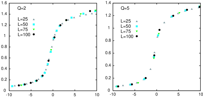
Figure 1: Scaling plots of the magnetization for $Q=2$ and $Q=5$. $\left\langle M\right\rangle L^{1/8}$ as function of $\beta^{\ast}L$. $\beta^{\ast}=\frac{\beta-\beta^{Q}_{c}}{\beta^{Q}_{c}}$ is the reduced inverse temperature.

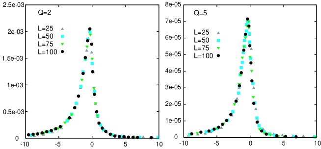
Figure 2: Scaling plots of the susceptibility $\left[M-\left\langle M\right\rangle\right]^{2}\times L^{-7/4}$ as function of $\beta^{\ast}L$, for $Q=2$ and $Q=5$ for different system sizes.

In the following we present computed mean values of the Euler characteristic and related Betti’s numbers per site and per color for several values of $Q$ as function of the inverse temperature $\beta$.

Periodic boundary conditions have been used which obviously lead to a symmetry between colors $a$ and$-a$. The equilibrium configuration presents a preference for positively or negatively oriented spins. We have chosen in the statistics, the first one, i.e. the one corresponding to $+Q$ boundary conditions.

Figure 3 shows the behaviour of the mean values of the global Euler characteristic $\chi_{\Lambda}$ and Betti’s numbers $\pi^{0}_{\Lambda}$ and $\pi^{1}_{\Lambda}$ as function of $\beta$ for $Q=1,2,5$ and $|\Lambda|=100^{2}$. Recall from (6) that $\pi^{0}_{\Lambda}(\beta)$ is nothing but the number of connected components of the complex and $\pi^{1}_{\Lambda}(\beta)$ is the number of independent cycles, i.e. the number of $1-$dimensional holes in the complex.

Seemingly, $\chi_{\Lambda}(\beta)$ appears as a decreasing function of $\beta$ and vanishes for $\beta>\beta_{c}$. The decrease of $\chi_{\Lambda}(\beta)$ for $\beta<\beta_{c}$ is associated both to a decrease of $\pi^{0}_{\Lambda}(\beta)$ and an increase of $\pi^{1}_{\Lambda}(\beta)$. In addition one observes that for $\beta>\beta_{c}$ these two quantities decrease and seem to compensate each other. This would explain the vanishing of $\chi_{\Lambda}(\beta)$ for $\beta\geqslant\beta_{c}$. As we shall see this compensation can be understood intuitively by looking at the behaviour of the colored Euler-Poincaré characteristic $\chi^{a}_{\Lambda}(\beta)$ and colored Betti’s numbers $\pi^{0,a}_{\Lambda}(\beta)$, $\pi^{1,a}_{\Lambda}(\beta)$, $a\in S_{Q}$, $Q=1,2,5$.

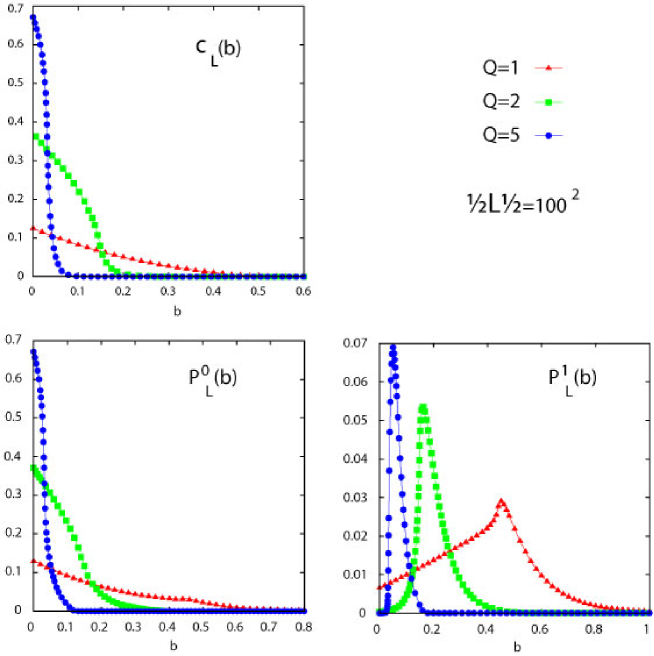
Figure 3: Mean values of the global Euler characteristic $\chi$ and global Betti’s numbers $\Pi_{0}$ and $\Pi_{1}$ for $Q=1,2,5$ and lattice size $|\Lambda|=100^{2}$.

Let us look at the Ising case $Q=1$ for which these quantities are presented in Figure 4. We observe that for $\beta<\beta_{c}$ the quantities $\chi^{a}_{\Lambda}(\beta)$, $\pi^{0,a}_{\Lambda}(\beta)$, $\pi^{1,a}_{\Lambda}(\beta)$ do not depend on colors $a=\pm 1$. However they exhibit a sharp transition in the color variable right at the critical point.

It is also seen that above $\beta>\beta_{c}$, $\pi^{0,+1}_{\Lambda}\simeq\pi^{1,-1}_{\Lambda}\simeq 0$ and $\pi^{1,+1}_{\Lambda}\simeq\pi^{0,-1}_{\Lambda}$. Therefore $\pi^{0}_{\Lambda}\simeq\pi^{1}_{\Lambda}$ which implies that in this range of temperature the global Euler characteristic vanishes. Alternatively the behaviour of the colored Betti’s numbers explain why $\chi^{+1}_{\Lambda}(\beta)\simeq-\chi^{-1}_{\Lambda}(\beta)$ which, in view of formula (13), gives also that the global Euler characteristic vanishes. These facts can be understood intuitively at low temperatures if one has in mind the usual picture of islands of $(-)$ inside a sea of $(+)$. Indeed, for such configurations, say $\boldsymbol{\sigma}_{\Lambda}$, one has $\boldsymbol{\pi}^{0,+1}_{\Lambda}(\boldsymbol{\sigma}_{\Lambda})\simeq\boldsymbol{\pi}^{1,-1}_{\Lambda}(\boldsymbol{\sigma}_{\Lambda})\simeq 1$ and each island gives a contribution $1$ to both $\boldsymbol{\pi}^{1,+1}_{\Lambda}(\boldsymbol{\sigma}_{\Lambda})$ and $\boldsymbol{\pi}^{0,-1}_{\Lambda}(\boldsymbol{\sigma}_{\Lambda})$.

On the other hand, when $\beta<\beta_{c}$ there exists only one (disordered) phase with independent colors. This corroborates the fact that $\chi^{a}_{\Lambda}(\beta)$, $\pi^{0,a}_{\Lambda}(\beta)$ and $\pi^{1,a}_{\Lambda}(\beta)$ do not rely on colors in this domain of temperature. In addition, the disorder increases when beta decreases, and in this domain of temperature it is natural to expect that the number of connected components of each color increases, while the number of independent cycles (of each color) decreases.

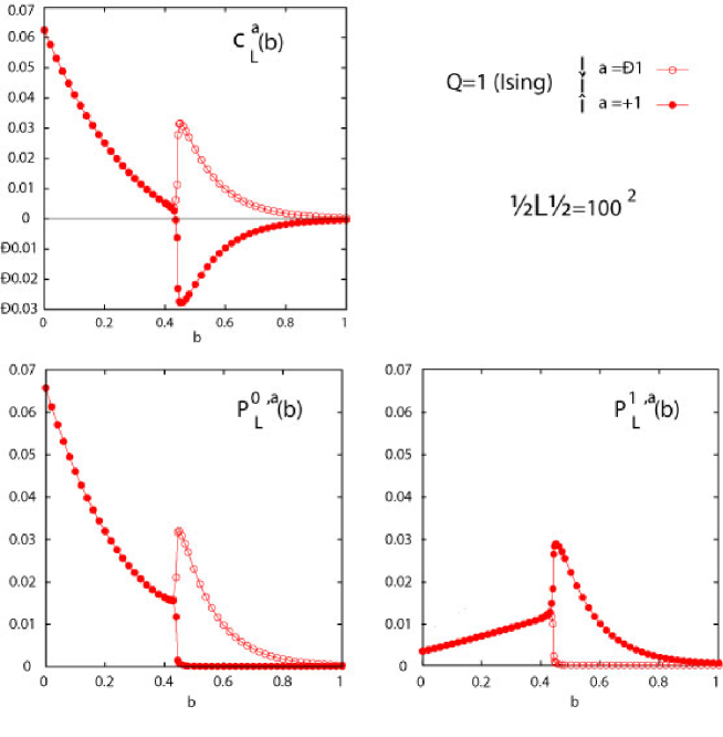
Figure 4: Mean values of the colored Euler characteristic $\chi^{a}(\beta)$ and Betti’s numbers $\pi^{0,a}(\beta)$ and $\pi^{1,a}(\beta)$ for $Q=1$ and $|\Lambda|=100^{2}$.

Figure 5 shows the results for the case $Q=2$ ($a=0,\pm 2$). Considering first the colors $a=\pm 2$, one can formulate the same reasoning as for the case $Q=1$. The quantities of interest behave similarly as before except for the amplitudes.

The color $a=0$ does not present any particular feature. $\pi^{1,0}_{\Lambda}(\beta)\simeq 0$ translates the fact that this color is dominated by the two extremal states $a=-2,+2$ for all values of $\beta$. This is reflected by noting that $\chi^{0}_{\Lambda}(\beta)\simeq\pi^{0,0}_{\Lambda}(\beta)$ in Figure 5.

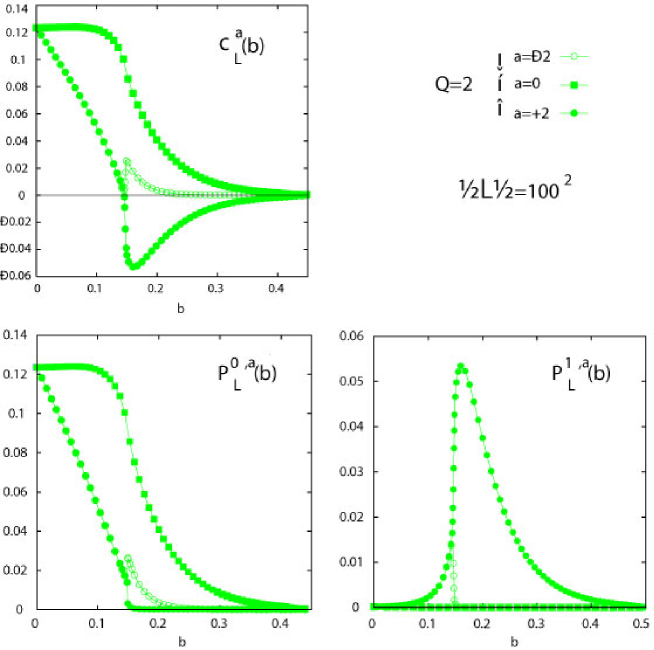
Figure 5: Mean values of the colored Euler characteristic $\chi^{a}(\beta)$ and Betti’s numbers $\pi^{0,a}(\beta)$ and $\pi^{1,a}(\beta)$ for $Q=2$ and $|\Lambda|=100^{2}$.

In Figure 6 we present our results for the case $Q=5$ ($a=\pm 5,\pm 3,\pm 1$). We observe that for $\beta>\beta_{c}$ the main contribution to the number of connected components comes from color $a=-3$.

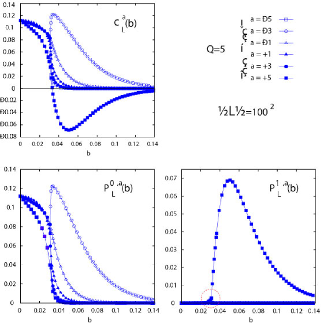
Figure 6: Mean values of the colored Euler characteristic $\chi^{a}(\beta)$ and Betti’s numbers $\pi^{0,a}(\beta)$ and $\pi^{1,a}(\beta)$ for $Q=5$ and $|\Lambda|=100^{2}$.

Figure 7 below gives an enlargement of Figure 6 showing the behavior of the other colors. Here also a sharp transition is observed at the critical point.

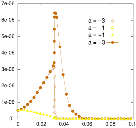
Figure 7: Enlargement of Figure 6 near the critical point.

All numerics have been performed with careful thermalization control (up to $5.10^{6}$ MC steps before measurements). Data simulation errors were controlled through binning analysis. In all figures, the error bars are smaller than the sizes of the symbols. The Hoshen-Kopelman cluster search algorithm [15] for colored connected components identification has been used.

4 Conclusion

In [6] we have already shown that for the Random Cluster Model, the mean value of the Euler-Poincaré characteristic with respect to the Fortuin-Kasteleyn measure exhibits a non trivial behaviour at the critical point. Namely, there we found that, in dimension $2$, it is either zero or discontinuous at the transition point.

Here, for the Ising model with arbitrary spins on $\mathbbm{Z}^{2}$, our numerics show that the topology of configurations reveals the signature of the phase transition. In particular this leads us to following conjecture

Conjecture: in the thermodynamic limit, $\chi_{\Lambda\uparrow\mathbbm{Z}^{2}}(\beta)>0$ for $\beta<\beta_{c}$ and $\chi_{\Lambda\uparrow\mathbbm{Z}^{2}}(\beta)=0$ for $\beta>\beta_{c}$.

We think that the vanishing of $\chi_{\Lambda\uparrow\mathbbm{Z}^{2}}(\beta)$ can be shown at large $\beta$ by perturbative Peierls type arguments in view of the expression (15) of the local Euler characteristic.

It would be interesting to study also these quantities in models with color symmetry like the Potts or Clock models [16].

Acknowledgments

Warm hospitality and Financial support from the BiBoS research Center, University of Bielefeld and Centre de Physique Théorique, CNRS Marseille are gratefully acknowledged. One of the authors, Ch. D., acknowledges financial support from the IRCSET embark-initiative postdoctoral fellowship scheme. We thank the referee for constructive remarks.

References

- [1] Serra J, image analysis and mathematical morphology, 1982 Academic Press, London.
- [2] Mecke K, morphology of spatial patterns : porous media, spinodal decomposition, and dissipative structures, 1997 Acta Physica Polonica B, 28 1747–1782.
- [3] Mecke K, exact moments of curvature measures in the boolean model, 2001 Acta Physica Polonica B, 102 1343–1381.
- [4] Winkler G, image analysis, Random Fields and Markov Chain Monte Carlo Springer, 2003.
- [5] Wagner H, Euler characteristic for archimedean lattices, 2000 Unpublished.
- [6] Blanchard Ph, Gandolfo D, Ruiz J, and Shlosman S, on the Euler–Poincaré characteristic of the random cluster model, 2003 Mark. Proc. Rel. Fields, 9 523.
- [7] Sykes M F and Essam J W, exact critical percolation probabilities for site and bond problems in two dimensions, 1964 J. Math. Phys. , 5 1117–1121.
- [8] Grimmet G, Percolation, 1999 Springer, 2nd edition.
- [9] Griffiths R B, rigorous results for Ising ferromagnet of arbitrary spins, 1969 J. Math. Phys., 10 1559.
- [10] Griffiths R B, correlations in Ising ferromagnets II., 1967 J. Math. Phys., 8 484–489.
- [11] Binder K, finite size scaling analysis of Ising model block distribution functions, 1981 Z. Phys. 43 119.
- [12] Nicolaides D and Bruce A D, universal configurational structure in two-dimensional scalar models, 1988 J. Phys. A: Math. Gen. 21 233–243.
- [13] Chen X S and Dohm V, nonuniversal finite–size scaling in anisotropic systems, 2004 Phys. Rev. E 70 056136.
- [14] Selke W and Shchur L N, critical Binder cumulant in two–dimensional anisotropic Ising models, 2005 J. Phys. A: Math. Gen. 38 L739–L744.
- [15] Hoshen J and Kopelman R, percolation and cluster distribution I., cluster multiple labeling technique and critical concentration algorithm, 1976 Phys. Rev. B, 14:3438.
- [16] work in progress.