Small parameter for lattice models with strong interaction

Abstract

Diagram series expansion for lattice models with a localized nonlinearity can be renormalized so that diagram vertexes become irreducible vertex parts of certain impurity model. Thus renormalized series converges well in the very opposite cases of tight and weak binding and pretends to describe in a regular way strong-correlated systems with localized interaction. Benchmark results for the classical $O(N)$ models on a cubic lattice are presented.

One of the key problems of the modern condensed-matter theoretical physics is the quest for a regular description of the strong correlations Fulde . Roughly speaking, correlations are strong if the nonlinearity and coupling are comparable, and therefore perturbative approaches make no sense.

Consider a lattice model with local coupling between cells with a nonlinearity localized inside each cell. In the two limit cases of the weak and tight binding a series expansion can be performed in powers of the respective small parameters Balesku . One of a few regular ways to handle the situation of crossover is to employ the concept of localized correlations. It basically means that interaction of each cell with the rest of the system can approximately be described as an interaction with certain non-correlated effective bath Cowley . The parameters of this bath are to be found self-consistently. If there is, say, one particle per cell, it means that real multi-site problem is approximated by much simpler single-site one (”impurity problem”). An example of such an approach is the mean-field description of the classical statistical ensembles of interacting particles. In this scheme, interaction of a particle with its fluctuating surrounding is replaced with interaction of a particle with a constant average field. There is a self-consistent equation for this field. An accuracy can be dramatically increased for change the mean-field by Gaussian-bath approximation. In this case, the surrounding is approximated by certain Gaussian ensemble. It is important that almost the same argumentation can be presented for very wide class of systems. Particularly, so-called dynamical mean-field theory (DMFT) for strongly interacting fermions is essentially a Gaussian-bath approximation DMFT .

Physically, Gaussian-bath approximation consists in the assumption that the irreducible part of high momenta is localized inside a single site. The strong point of this assumption is that it is valid for several very different limits for systems with localized nonlinearity. The approximation reproduces leading-order results of the weak- and tight-binding series expansion simultaneously. Indeed, if the nonlinearity is small, the perturbation theory explicitly says that correlations are localized in the first-order of weak-binding approximation. On the other hand, if coupling goes to zero, sites become almost isolated and correlations are obviously localized, no matter how strong the nonlinearity is. Once the two opposite limits are described well, their crossover can be expected to be also somehow depicted. There is some more justifications for the scheme, particularly it becomes exact for a system of an infinite dimensionality.

Since an analysis of proper impurity problem gives a good understanding of the properties of strongly-correlated systems, it is desirable to construct a perturbation theory starting from the solution of an impurity problem as a zeroth approximation. A theory of this kind is presented in this paper for lattice models with a localized nonlinearity. We exactly renormalize diagram expansion so that diagram vertexes become irreducible vertex parts of certain impurity problem. An important peculiarity of the proposed approach is that a good convergence is achieved both in tight-binding and weak-binding situations. As an example, we present the results obtained for quantum Ising model in a transverse field.

We consider statistics of the real vector field $\phi$ on a discrete lattice with a localized nonlinearity $\Theta(\phi)$ and the dispersion law $\Omega$. In general, lattice potential can depend on a number of the lattice site. Through the article we number sites by $x$ whereas components of the on-site field $\phi_{x}$ are numbered by $j$, statistical average is denoted by triangle brackets:

$$<...>=Z^{-1}\int...~{}e^{-\beta E(\phi)}[D\phi]$$ (1)

$$Z=\int e^{-\beta E(\phi)}[D\phi]$$

$$E(\phi)=\sum_{x}\Theta_{x}(\phi_{x})+\frac{1}{2}(\phi\Omega\phi).$$

Scalar product $(\phi\Omega\phi)$ is a sum over both indices: $\sum_{xx^{\prime}jj^{\prime}}\phi_{xj}\Omega_{xx^{\prime}jj^{\prime}}\phi_{x^{\prime}j^{\prime}}$; below we also use external product denoted by the dot: $\phi\cdot\phi$. The notation $(\phi_{x}\Omega_{xx}\phi_{x})$ is used for a scalar product in the on-site subspace: $(\phi_{x}\Omega_{xx}\phi_{x})\equiv\sum_{jj^{\prime}}\phi_{xj}\Omega_{xxjj^{\prime}}\phi_{xj^{\prime}}$.

Consider an auxiliary ensemble with energy

$$E^{aux}(\phi)=\sum_{x}\Theta_{x}(\phi_{x})+\frac{1}{2}\left(\phi A\phi\right)+(\phi^{0}(\Omega-A)\phi).$$ (2)

We introduced here vector quantity $\phi^{0}$ and a Hermitian tensor $A$ having non-zero terms only at the same $x$-indices: $A_{xx^{\prime}}=0$ for $x\neq x^{\prime}$ (through the text we call such quantities ’$x$-diagonal’). The values of $A$ and $\phi^{0}$ are not specified for a while.

Since $A$ is $x$-diagonal, site oscillators of the auxiliary ensemble are uncoupled (one can see that $E^{aux}(\phi)$ splits to a sum of independent single-site energies). Thus, properties of the auxiliary system at each site can be obtained as a solution of a single-site impurity problem.

Denote an average over the auxiliary ensemble by overline and introduce normalized two-point correlator and higher-order irreducible vertex parts at the sites of auxiliary system:

$$g_{12}=\beta\left(\overline{\phi_{1}\phi_{2}}-\overline{\phi_{1}}~{}\overline{\phi_{2}}\right)$$ (3)

$$\gamma^{(3)}_{1^{\prime}2^{\prime}3^{\prime}}=-\beta^{3}g_{1^{\prime}1}^{-1}g_{2^{\prime}2}^{-1}g_{3^{\prime}3}^{-1}\left(\overline{\phi_{1}\phi_{2}\phi_{3}}-\overline{\phi_{1}\phi_{2}}~{}\overline{\phi_{3}}-\overline{\phi_{1}\phi_{3}}~{}\overline{\phi_{2}}-\overline{\phi_{2}\phi_{3}}~{}\overline{\phi_{1}}+2\overline{\phi_{1}}~{}\overline{\phi_{2}}~{}\overline{\phi_{3}}\right)$$

$$\gamma^{(n)}_{1^{\prime}..n^{\prime}}=(-\beta)^{n}g_{1^{\prime}1}^{-1}...g_{n^{\prime}n}^{-1}\cdot({\rm irreducible~{}part~{}of~{}the}~{}n{\rm-th~{}moment}).$$

To simplify the notation, we omit site index $x$ and write numbers as subscripts for the on-site coordinates here.

It should be noted that mean-field and Gaussian-bath approximations can be understood as approximations of the system (1) by (2) with a self-consistent requirement $\phi^{0}=\overline{\phi}$ and certain choice of $A_{xx}$. Indeed, to obtain the mean-field scheme, one should, first, replace all $\phi$ in $E(\phi)$ with its average for all cells except just a single one, and, second, use an average over this particular cell as a guess for $<\phi>$. It is easy to check that the mean-field corresponds to the simple choice $A_{xx}=\Omega_{xx}$. Gaussian-bath approximation also reduces the system to a single-site problem. The difference is that the remaining degrees of freedom are not frozen in its average positions, but approximated with harmonic oscillators, forming Gaussian bath. These Gaussian degrees of freedom can be integrated out, giving again single-site energy like in (2) with certain $A$. An approximation for the single-site system by a harmonic oscillator can be found from the requirement that the approximation mimics $\overline{\phi_{x}}$ and $g_{xx}$. Thus obtained parameters of harmonic oscillators are to be used as in the next iteration of the self-consistent loop as parameters of the oscillators forming the bath. These iterations converge to the point where $x$-diagonal part of the tensor $\left(g+(\Omega-A)^{-1}\right)^{-1}$ vanish. This is in fact a condition for $A$ of the Gaussian-bath approximation.

The aim of this paper is to express averages (1) via $\overline{\phi}$, $g$ and $\gamma^{(n)}$ by certain regular series. The quantities $A$ and $\phi_{0}$ will determined by certain self-consistent conditions.

First, we would like to introduce the ”dual” variables $f$. Let us consider the basis where $g(\Omega-A)g$ is diagonal and label the states in this basis by $p$. Define the integration $\int[Df]\equiv\int df_{p_{1}}...\int df_{p_{n}}...$ in such a way that the path of integration in each integral depends on a sign of diagonal element $(g(\Omega-A)g)_{pp}$: $f_{p}$ goes from $-\infty$ to $\infty$ for $(g(\Omega-A)g)_{pp}<0$ and from $-i\infty$ to $i\infty$ overwise. With thus defined $\int[Df]$, the following identity holds:

$$e^{-\frac{1}{2}\beta\left((\phi-\phi^{0})(\Omega-A)(\phi-\phi^{0})\right)}=({\rm factor})\times\int[Df]e^{-\beta\left(((\phi-\phi^{0})g^{-1}f)-\frac{1}{2}(f(g(\Omega-A)g)^{-1}f)\right)}.$$ (4)

In fact, the path of integration over $f_{p}$ is chosen to deliver the convergence of integrals here. After this identity is applied, partition function takes the form

$$Z=\int[D\phi]\int[Df]e^{-\beta E(\phi,f)}$$ (5)

$$E(\phi,f)=E^{aux}(\phi)+((\phi-\phi^{0})g^{-1}f)-\frac{1}{2}(f(g(\Omega-A)g)^{-1}f),$$

A set of exact relations between the averages over initial and dual ensemble can be established by the integration by parts in (5) with respect to $f$. Particularly,

$$g(\Omega-A)<\phi-\phi^{0}>=<f>;$$ (6)

$$g(\Omega-A)<(\phi-\phi^{0})\cdot(\phi-\phi^{0})>(\Omega-A)g=<f\cdot f>+\beta^{-1}g(\Omega-A)g.$$

The idea of an introduction of new variables is that energy (5) does not contain direct coupling between different sites for the initial variable $\phi$, since $(\phi g^{-1}f)=\sum_{x}(\phi_{x}(g^{-1}f)_{x})$. Therefore $\phi_{x}$ can be integrated out at each site, yielding an an expression for the energy in dual variables $E(f)$:

$$E(f)=\sum_{x}V_{x}(f_{x})+\frac{1}{2}\left(f\tilde{\Omega}f\right)$$ (7)

$$\tilde{\Omega}=-g^{-1}-g^{-1}(\Omega-A)^{-1}g^{-1}$$

This expression is formally very similar to an initial system (1). Physical difference comes, first, from the possibility to choose $A$ and $\phi^{0}$ in certain optimal way, and, second, from the the non-trivial way of integration over $f$ so that $f$ has an imaginary part. In particular, $<f_{xj}^{2}>$ can be negative or equal zero.

Properties of the dual potential $V(f)$ are determined by the cumulant expansion (2) for an auxiliary system. The last term in (7) is chosen in such a way that the second derivative of $V$ vanishes; other derivatives are $V^{(1)}=(\overline{\phi}-\phi^{0})g^{-1}$ and $-\beta V^{(n)}=\gamma^{(n)}$ for $n\geq 3$. To describe effects due to nonlinearity, we introduce tensor $\Sigma^{\prime}$ defined by equation

$$<\phi\cdot\phi>=\beta^{-1}(g^{-1}+\Omega-A+\Sigma^{\prime})^{-1},$$ (8)

so that $\Sigma^{\prime}$ describes a non-local contribution to the self-energy of the initial system (1). It follows from the second line of (6) that dual two-point correlator can be expressed via $\Sigma$ as follows:

$$<f\cdot f>=g\frac{-\beta^{-1}}{(g^{-1}-\Sigma^{\prime})^{-1}+(\Omega-A)^{-1}}g.$$ (9)

All expressions presented above are exact. Now, we construct a perturbation theory resulting from the series expansion in powers of $V$. Terms of these series can be expressed by the diagrams with $\gamma^{(n)}$ standing at vertexes connected with lines carrying dual two-point correlator $<f\cdot f>$. We consider the series for $\Sigma^{\prime}$. It can be found from the expansion of the left- and right-hand side of (9) in powers of $V$ and $\Sigma^{\prime}$, respectively. Some of those diagrams are presented in Figure 1. Each diagram is accompanied by an additional factor $-\beta^{-1}$ and a numerical coefficient. It can be found from the above-mentioned expansion of (9).

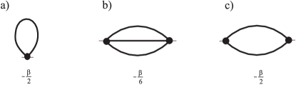
Figure 1: Diagrams contributing $\Sigma^{\prime}$ and corresponding coefficients. Diagram (a) is small if condition (11) is fulfilled. Diagrams (b) and (c) describe av $\alpha^{2}$ correction to $\Sigma^{\prime}$; diagram (c) vanishes for an unordered state of $O(N)$ model.

Formally, single-lag vertexes can occur in the diagrams due to the presence of $V^{(1)}$ in the dual energy (7). We require such $\phi^{0}$ that $<f>=0$ to get rid of them. Then the first line of (6) requires

$$<\phi>=\phi^{0}.$$ (10)

Since $\gamma^{(n)}$ of any order can in principle appear in the series, a formal small parameter should be introduced to group the terms properly. Consider a special case of a scalar field with small nonlinearity: $U(\phi)=\alpha\phi^{4}$, $\alpha\to+0$. Estimate how $\alpha$ appears in high derivatives of $V(f)$: $\gamma^{(2n)}\propto\alpha^{n}$ and $\gamma^{(2n-1)}\propto\alpha^{n}\phi_{0}$. We propose to group diagrams with respect to their formal smallness in powers of $\alpha$. This is clearly a good choice for a weak-binding limit. Consider the opposite case of tight-binding $\Omega\to 0$ and suppose that our choice of $A$ delivers also $(A-\Omega)\to 0$ (note that mean-field and Gaussian-bath schemes satisfy this condition). It is obvious from (7) that bare two-point correlator appears to be a small quantity in this case. Since the number of lines in a diagram is roughly proportional to its $\alpha$-order, $\alpha$ again appears to be a good small parameter. We conclude that series expansion converges well both in tight-binding and weak-binding limits and therefore expect that the theory is suitable for a crossover situation.

Formally, series expansion can be constructed for any $A$, but an appropriate choice should result to better convergence. It is useful to require

$$\beta^{-1}g=<(\phi-\phi_{0})\cdot(\phi-\phi_{0})>_{xx}.$$ (11)

One can formally obtain Gaussian-bath approximation as a result of Gaussian approximation for $<f\cdot f>$ in (9), combined with requirements (10,11). Gaussian approximation means $\alpha^{0}$ order of the theory. Higher terms of an expansion in powers of $\alpha$ improve the result and, in particular, bring non-local correlations on the scene.

To demonstrate capabilities of the method and to give more technical details, we present here the results obtained in an $\alpha^{2}$-approximation for classical $O(N)$ models at 3D cubic lattice with the nearest-neighbor coupling. Potential energy is

$$-\sum_{<xx^{\prime}>}(\phi_{x}\phi_{x^{\prime}}),$$ (12)

where $\phi_{x}$ is an $N$-component vector of the constrained length $||\phi_{x}||^{2}=(\phi_{x}\phi_{x})=N$. In the previous notation, dispersion law is $\Omega_{k}=-(\cos k_{x}+\cos k_{y}+\cos k_{z})$, whereas the constrain makes the system nonlinear. Sum is over all pairs of the nearest neighbors. Cases of $N=1,2,3$ correspond to Ising, $xy$, and Heisenberg models, respectively. In three dimensions, system (12) shows a second-order phase transition at finite temperature for $N$. The model is extensively studied. One can note Monte Carlo simulations HeisenbergMC ; Ising , high-temperature expansion HT (in our terminology, this is in fact tight-binding approach), renormalisation-group methods RG etc. Here we do not pretend to obtain something new for the model itself. It is used to check if the method works for a realistic system.

For simplicity, let us consider an unordered state $<\phi>=0$, so that only even-lag vertexes appear in diagrams, $\gamma^{(2n+1)=0}$. It can be easily obtained that $g_{12}=\beta^{-1}\delta_{12}$ (irrespective on $N$) and $\gamma^{(4)}_{1234}=\gamma_{N}(\delta_{12}\delta_{34}+\delta_{13}\delta_{24}+\delta_{14}\delta_{23})$ with $\gamma_{N=1}=-2/3,\gamma_{N=2}=-1/2,\gamma_{N=3}=-2/5$. Here $\delta$ is a Kronecker delta. Tensor structure of $g$, $\gamma^{(4)}$, as well as $A$, corresponds to the $O(N)$ symmetry of the problem.

The self-consistent equation for $a$ follows from (8) and (11):

$$g=\frac{1}{(2\pi)^{3}}\int\frac{d^{3}k}{g^{-1}+\Omega_{k}+\Sigma^{\prime}-A}$$ (13)

Technically, this equation can be solved iteratively, similarly to DMFT-loop technique DMFT . Start from certain guess for $A$ and $\Sigma^{\prime}$. For a general case, one should calculate $g(A)$ and $\gamma^{(n)}(A)$ at this point, but for a particular model (12) it is not necessary as $g$ and $\gamma$ do not depend on $A$, because of the constrain $||\phi_{x}||^{2}=N$. Calculate $<f\cdot f>$ from (9), given $g,A$, and $\Sigma^{\prime}$. For thus obtained $<f\cdot f>$ and $\gamma^{(n)}$, calculate new guess for $\Sigma^{\prime}$ for a given order in $\alpha$ (see below expressions for $\Sigma^{\prime}$ up to $\alpha^{2}$). Finally calculate the right-hand side of (13), given $g,A$, and new $\Sigma^{\prime}$. Denote the obtained value by $\tilde{g}$ and take the quantity $A+\xi(g^{-1}-\tilde{g}^{-1})$ as new guess for $A$, where $\xi\lesssim 1$ is a numerical factor. Repeat the loop for new $A$ and $\Sigma^{\prime}$. For properly chosen initial guess and value of $\xi$ iterations converge to a fixed point satisfying equation (12).

Gaussian-bath approximation corresponds to an assumption $\Sigma^{\prime}=0$. Corrections are given by the diagrams presented in Figure 1. Lines in these diagrams are thick, i.e. they correspond to the renormalized correlator $<f\cdot f>$. First-order correction would be given by a simple loop shown as diagram (a) in Figure 1. This diagram corresponds to formula $-\frac{1}{2\beta}\gamma^{(4)}<f_{x}\cdot f_{x}>$. It is however absent, because $<f_{x}\cdot f_{x}>$ equals zero in Gaussian-bath approximation, as it can be obtained from (6) and (13). So the correction starts actually from $\alpha^{2}$ terms.

Strictly speaking, once high-order corrections are taken into account, $<f_{x}\cdot f_{x}>$ does not vanish anymore. But it remains small. It can be shown that simple loops does not appear in diagrams up to $\alpha^{3}$ order. Consequently, second-order correction to $\Sigma^{\prime}$ can be described by just a single diagram (b) drawn in Figure 1, so that $\Sigma^{\prime}_{xx^{\prime}}=-\frac{1}{6\beta}\gamma^{2}<f_{x}\cdot f_{x^{\prime}}>^{3}$. After the sum over internal indices is taken, it gives $\Sigma^{\prime}_{xx^{\prime}}=-\beta^{-1}\gamma^{2}(1+N/2)f_{x,x^{\prime}}^{3}$, where $f_{x,x^{\prime}}$ is a diagonal element of the dual correlator.

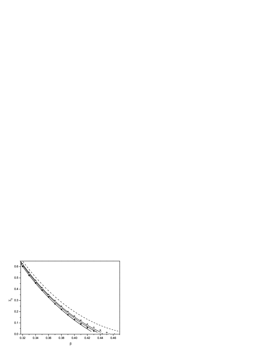
Figure 2: Effective soft-mode dispersion for $O(N)$ model at $N=1,2,3$. Dashed line: Gaussian-bath approximation. Solid lines: results for the $\alpha^{2}$-scheme, from bottom to top: $N=1$ (Ising), $N=2$ (xy), and $N=3$ (Heisenberg). In a narrow region near critical point the iteration procedure did not converge, and the lines are not drawn. Symbols are numerical data for $N=1,2,3$: respectively solid circles, open circles and crosses. Dotted line is a fit corresponding to a ‘purely critical’ behavior of $<\phi\cdot\phi>$ in Ising model.

Figure 2 shows data for the effective soft-mode dispersion $\Sigma_{0}\equiv(\beta<\phi_{k=0}\cdot\phi_{k=0}>)^{-1}$. Dots are numerical data. Data for the lines are obtained by formula $\Sigma_{0}=g^{-1}+\Omega_{k=0}+\Sigma^{\prime}-A$. Iteration procedure converges well everywhere except very narrow regions near critical point. Since we were not interested in a description of the critical point itself, we did not put special attention to the source of this divergence.

Gaussian-bath approximation predicts the same dependence for any $N$, as one can observe from (13) with $\Sigma^{\prime}=0$. This is a serious qualitative drawback, although the quantitative accuracy is not so bad. So, the dependence of $\Sigma_{0}$ on $N$ in the model is related with a non-local part of correlations, and should be described by higher terms of $\alpha$-corrections. Indeed, $\alpha^{2}$-correction describes the dependence $\Sigma_{0}(N)$ well. There is also a dramatic increase of the accuracy in the $\alpha^{2}$ curves.

For the broken-symmetry state, the theory can be constructed in a very similar manner. Iteration loop now includes also a modification of $\phi^{0}$ to fulfill the condition (10) at a fixed point. Diagram (c) from Figure 1 appears due to the presence of $\gamma^{(3)}$. We do not show numerical results here, because they are very similar to what we obtain for the unordered state.

The entire plot range of Figure 2 lies within a critical region. For example, all points for Ising model obey critical scaling law $<\phi_{k=0}^{2}>\propto(\beta-\beta_{c})^{1.24}$ with a good accuracy, as the dashed line shows. Thus the theory performs well deep inside the critical region. However, the very vicinity of the critical point is not correctly described, because we work with perturbation theory of a finite order. It would be worth to construct a renormalization-group theory based on the presented perturbation approach. An attempt to construct a primitive approach of this kind starting from mean-field theory was performed several years ago dualRG .

There is a comment about an applicability of other approximation schemes. The system is strongly nonlinear, so weak-binding approximation is clearly not valid here. On the other hand, tight-binding description of a low order fails near the phase transition point because of the critical increase of the correlation length. For example, second order of the tight-binding series gives $\Sigma_{0}=\beta^{-1}(1+4\beta)^{-1}$. This is very inaccurate; corresponding curve simply lies out of the plot range of Figure 2. More sophisticated schemes, for example, cumulant expansion, also require much higher order to achieve an accuracy comparable with the presented $\alpha^{2}$ results. It is also important to recall that Gaussian-bath approximation becomes exact in the limit $N\to\infty$, and $1/N$ expansion can be constructed at this point 1/N . But $1/N$ approach is essentially based on a very particular $O(N)$ symmetry of system (12). Contrary, our method is developed for a general case and does not require any special symmetry.

In conclusion, we presented an exact renormalization of the diagram-series expansion in terms of the self-consistent impurity model. Renormalized vertexes are irreducible vertex parts of the impurity model. There is an explicit small parameter in the theory for weak-binding and tight-binding limit. A worked example of an $\alpha^{2}$-approximation for simple 3D models demonstrates that the method performs well for a strong-correlated situation. The example models were chosen because of the physical simplicity; the method itself looks rather general. It would be particularly important to extend it to the systems of identical quantum particles. Another challenge is a construction of renormalization-group theory based on the method.

The work was supported by Dynasty foundation and NWO grant 047.016.005. Author is grateful to M.I. Katsnelson and O.I.Loiko for their interest to this work.

References

- (1) P.Fulde, Electron Correlations in Molecules and Solids, Springer, Berlin, 2002
- (2) R. Balesku, Equilibrium and Nonequilibrium Statistical Mechanics, Wiley, New York, 1975.
- (3) A.D. Bruce and R.A. Cowley Structural phase transitions, Taylor and Francis Ltd., London, 1981.
- (4) A. Georges, G. Kotliar, W. Krauth, and M.J. Rozenberg, Rev. Mod. Phys. 68, 13 (1996).
- (5) P. Peczak, A.L. Ferrenberg, and D.P. Landau, Phys. Rev. B 43, 6087 (1991).
- (6) A. M. Ferrenberg and D. P. Landau, Phys. Rev. B 44, 5081 (1991).
- (7) M. Campostrini, A. Pelissetto, P. Rossi, and E. Vicari, Phys. Rev. E 65, 066127 (2002).
- (8) A. Pelissetto and E. Vicari, Physics Reports 368, 549 (2002).
- (9) H.Li, T. Chen, Z. Phys. B 100, 283 (1996).
- (10) A.N. Rubtsov, Phys. Rev. B 66,052107-1 (2002).
- (11) Y. Okabe, M. Oku, R. Abe, Progress of Theoretical Physics 59, 1825 (1978).