One-loop approximation for the Hubbard model

Abstract

The diagram technique for the one-band Hubbard model is formulated for the case of moderate to strong Hubbard repulsion. The expansion in powers of the hopping constant is expressed in terms of site cumulants of electron creation and annihilation operators. For Green’s function an equation of the Larkin type is derived and solved in a one-loop approximation for the case of two dimensions, nearest-neighbor hopping and half-filling. The obtained four-band structure of the spectrum and the shapes of the spectral function are close to those observed in Monte Carlo calculations. It is shown that the maxima forming the bands are of a dissimilar origin in different regions of the Brillouin zone.

I Introduction

Systems with strong electron correlations which, in particular, cuprate perovskites belong to are characterized by a Coulomb repulsion that is comparable to or larger than hopping constants. One of the simplest models for the description of such systems is the Hubbard model Gutzwiller ; Hubbard63 ; Kanamori with the Hamiltonian

$$H=\sum_{\bf nm\sigma}t_{\bf nm}a^{\dagger}_{\bf n\sigma}a_{\bf m\sigma}+\frac{U}{2}\sum_{\bf n\sigma}n_{\bf n\sigma}n_{\bf n,-\sigma},$$ (1)

where $t_{\bf nm}$ is the hopping constants, the operator $a^{\dagger}_{\bf n\sigma}$ creates an electron on the site n with the spin projection $\sigma=\pm 1$, $U$ is the on-site Coulomb repulsion, the electron number operator $n_{\bf n\sigma}=a^{\dagger}_{\bf n\sigma}a_{\bf n\sigma}$. In the case of strong electron correlations, $U\gtrsim|t_{\bf nm}|$, it is reasonable to use a perturbation expansion in powers of the hopping constants for investigating Hamiltonian (1). Apparently the first such expansion was considered in Ref. Hubbard66, . The further development of this approach was given in Refs. Westwanski, ; Stasyuk, ; Zaitsev, ; Izyumov, ; Ovchinnikov, where the diagram technique for Hubbard operators was developed and used for investigating the Mott transition, the magnetic phase diagram and the superconducting transition in the Hubbard model.

The rules of the diagram technique for Hubbard operators are rather intricate. Besides, these rules and the graphical representation of the expansion vary depending on the choice of the operator precedence. The diagram technique suggested in Refs. Vladimir, ; Metzner, ; Moskalenko, ; Pairault, is free from these defects. In this approach the power expansion for Green’s function of electron operators $a_{\bf n\sigma}$ and $a^{\dagger}_{\bf n\sigma}$ is considered and the terms of the expansion are expressed as site cumulants of these operators. Based on this diagram technique the equations of the Larkin type Larkin for Green’s function were derived. Vladimir ; Moskalenko ; Pairault

However, the application of this approach runs into problems. In particular, at half-filling the spectral weight appears to be negative near frequencies $\omega_{d}=\pm\frac{U}{2}$. Pairault This drawback is connected with divergencies in cumulants at these frequencies. As can be seen from formulas given below, all higher-order cumulants have such divergencies at $\omega_{d}$ with sign-changing residues, which are expected to compensate each other in the entire series. If, as in Ref. Pairault, , only some subset of diagrams is taken into account the divergencies of different orders can be compensated only accidentally. On the other hand, at frequencies neighboring to $\omega_{d}$ cumulants are regular. If a selected subset of diagrams is expected to give a correct estimate of the entire series for these frequencies the values at $\omega_{d}$ can be corrected by an interpolation using results for the regular regions. This procedure is applied in the present work where the one-loop approximation is used – as irreducible diagrams in Larkin’s equation those appearing in the first two orders of the perturbation expansion are adopted. One of these diagrams contains a loop formed by a hopping line. It is shown that for the case of a square lattice, nearest-neighbor hopping and half-filling the electron spectrum consists of four bands. These band structure and the calculated shapes of the electron spectral function are close to those obtained in Monte-Carlo calculations Moreo ; Preuss ; Grober and recently in the cluster perturbation Dahnken and the two-particle self-consistent Tremblay calculations. It is shown also that the maxima forming the bands are of a dissimilar origin in different regions of the Brillouin zone.

In the following section the perturbation expansion for the electron Green’s function is formulated in the form convenient for calculations and Larkin’s equation is derived. In Sec. III the equations of the previous section are used for calculating the spectral function and the obtained results are discussed. Concluding remarks are presented in Sec. IV.

II Diagram technique

We consider Green’s function

$$G({\bf n\tau,n^{\prime}\tau^{\prime}})=\langle{\cal T}\bar{a}_{\bf n^{\prime}\sigma}(\tau^{\prime})a_{\bf n\sigma}(\tau)\rangle,$$ (2)

where the angular brackets denote the statistical averaging with the Hamiltonian ${\cal H}=H-\mu\sum_{\bf n\sigma}n_{\bf n\sigma}$, $\mu$ is the chemical potential, ${\cal T}$ is the time-ordering operator which arranges other operators from right to left in ascending order of times $\tau$, $a_{\bf n\sigma}(\tau)=\exp({\cal H}\tau)a_{\bf n\sigma}\exp(-{\cal H}\tau)$ and $\bar{a}_{\bf n\sigma}(\tau)=\exp({\cal H}\tau)a^{\dagger}_{\bf n\sigma}\exp(-{\cal H}\tau)$. Choosing

$$H_{0} = \frac{U}{2}\sum_{\bf n\sigma}n_{\bf n\sigma}n_{\bf n,-\sigma}-\mu\sum_{\bf n\sigma}n_{\bf n\sigma},$$

$$H_{1} = \sum_{\bf nm\sigma}t_{\bf nm}a^{\dagger}_{\bf n\sigma}a_{\bf m\sigma}$$

as the unperturbed Hamiltonian and the perturbation, respectively, and using the known Abrikosov expansion for the evolution operator we get

$$G({\bf n^{\prime}\tau^{\prime},n\tau}) = \sum_{k=0}^{\infty}\frac{(-1)^{k}}{k!}\int\!\ldots\!\int_{0}^{\beta}d\tau_{1}\ldots d\tau_{k}$$ (4)

$$\times \sum_{{\bf n}_{1}{\bf n}^{\prime}_{1}\sigma_{1}}\!\!\ldots\!\!\sum_{{\bf n}_{k}{\bf n}^{\prime}_{k}\sigma_{k}}t_{{\bf n}_{1}{\bf n}^{\prime}_{1}}\ldots t_{{\bf n}_{k}{\bf n}^{\prime}_{k}}$$

$$\times \langle{\cal T}\bar{a}_{\bf n^{\prime}\sigma}(\tau^{\prime})a_{\bf n\sigma}(\tau)\bar{a}_{{\bf n}^{\prime}_{1}\sigma_{1}}(\tau_{1})a_{{\bf n}_{1}\sigma_{1}}(\tau_{1})\ldots$$

$$\times \bar{a}_{{\bf n}^{\prime}_{k}\sigma_{k}}(\tau_{k})a_{{\bf n}_{k}\sigma_{k}}(\tau_{k})\rangle_{0c},$$

where $\beta=1/T$ is the inverse temperature, the subscript “0” near the angular bracket indicates that the averaging and time dependencies of operators are determined with the Hamiltonian $H_{0}$. The subscript “c” indicates that terms which split into two or more disconnected averages have to be dropped out.

The Hamiltonian $H_{0}$ is diagonal in the site representation. Therefore the average in the right-hand side of Eq. (4) splits into averages belonging to separate lattice sites. To be nonzero these latter averages have to contain equal number of creation and annihilation operators. Let us consider the average which appears in the first order: $\langle{\cal T}\bar{a}_{\bf n^{\prime}\sigma}(\tau^{\prime})a_{\bf n\sigma}(\tau)\bar{a}_{{\bf n}^{\prime}_{1}\sigma_{1}}(\tau_{1})a_{{\bf n}_{1}\sigma_{1}}(\tau_{1})\rangle$ (for short here and below subscripts “0” and “c” are omitted). For this average to be nonvanishing operators have to belong either to the same site or to two different sites,

$$\langle{\cal T}\bar{a}_{\bf n^{\prime}\sigma}(\tau^{\prime})a_{\bf n\sigma}(\tau)\bar{a}_{{\bf n}^{\prime}_{1}\sigma_{1}}(\tau_{1}^{\prime})a_{{\bf n}_{1}\sigma_{1}}(\tau_{1})\rangle=$$

$$\quad\langle{\cal T}\bar{a}_{\bf n\sigma}(\tau^{\prime})a_{\bf n\sigma}(\tau)\bar{a}_{{\bf n}\sigma_{1}}(\tau_{1}^{\prime})a_{{\bf n}\sigma_{1}}(\tau_{1})\rangle\delta_{\bf nn^{\prime}}\delta_{{\bf nn}_{1}^{\prime}}\delta_{{\bf nn}_{1}}$$

$$\quad+\langle{\cal T}\bar{a}_{\bf n\sigma}(\tau^{\prime})a_{\bf n\sigma}(\tau)\rangle\langle{\cal T}\bar{a}_{{\bf n}_{1}\sigma_{1}}(\tau_{1}^{\prime})a_{{\bf n}_{1}\sigma_{1}}(\tau_{1})\rangle$$

$$\quad\quad\times\delta_{\bf nn^{\prime}}\delta_{{\bf n}_{1}{\bf n}_{1}^{\prime}}(1-\delta_{{\bf nn}_{1}})$$

$$\quad-\langle{\cal T}\bar{a}_{{\bf n}_{1}\sigma}(\tau^{\prime})a_{{\bf n}_{1}\sigma_{1}}(\tau_{1})\rangle\langle{\cal T}\bar{a}_{{\bf n}\sigma_{1}}(\tau_{1}^{\prime})a_{\bf n\sigma}(\tau)\rangle$$

$$\quad\quad\times\delta_{{\bf n^{\prime}n}_{1}}\delta_{{\bf nn}_{1}^{\prime}}(1-\delta_{{\bf nn}_{1}}).$$

The multiplier $1-\delta_{{\bf nn}_{1}}$ ensures that ${\bf n}\neq{\bf n}_{1}$ in the two last terms (the case ${\bf n}={\bf n}_{1}$ is taken into account by the first term in the right-hand side). After the rearrangement of the terms we find

$$\langle{\cal T}\bar{a}_{\bf n^{\prime}\sigma}(\tau^{\prime})a_{\bf n\sigma}(\tau)\bar{a}_{{\bf n}^{\prime}_{1}\sigma_{1}}(\tau_{1}^{\prime})a_{{\bf n}_{1}\sigma_{1}}(\tau_{1})\rangle=$$

$$\quad K_{2}(\tau^{\prime}\sigma,\tau\sigma,\tau^{\prime}_{1}\sigma_{1},\tau_{1}\sigma_{1})\delta_{\bf nn^{\prime}}\delta_{{\bf nn}_{1}^{\prime}}\delta_{{\bf nn}_{1}}$$

$$\quad+K_{1}(\tau^{\prime}\sigma,\tau\sigma)K_{1}(\tau^{\prime}_{1}\sigma_{1},\tau_{1}\sigma_{1})\delta_{\bf nn^{\prime}}\delta_{{\bf n}_{1}{\bf n}^{\prime}_{1}}$$

$$\quad-K_{1}(\tau^{\prime}\sigma,\tau_{1}\sigma_{1})K_{1}(\tau^{\prime}_{1}\sigma_{1},\tau\sigma)\delta_{{\bf n^{\prime}n}_{1}}\delta_{{\bf nn}^{\prime}_{1}},$$

where

$$K_{1}(\tau^{\prime}\sigma^{\prime},\tau\sigma)=\langle{\cal T}\bar{a}_{\sigma}(\tau^{\prime})a_{\sigma}(\tau)\rangle\delta_{\sigma\sigma^{\prime}},$$

$$K_{2}(\tau^{\prime}\sigma,\tau\sigma,\tau^{\prime}_{1}\sigma_{1},\tau_{1}\sigma_{1})=$$

$$\quad\langle{\cal T}\bar{a}_{\sigma}(\tau^{\prime})a_{\sigma}(\tau)\bar{a}_{\sigma_{1}}(\tau^{\prime}_{1})a_{\sigma_{1}}(\tau_{1})\rangle$$ (5)

$$\quad-K_{1}(\tau^{\prime}\sigma,\tau\sigma)K_{1}(\tau^{\prime}_{1}\sigma_{1},\tau_{1}\sigma_{1})$$

$$\quad+K_{1}(\tau^{\prime}\sigma,\tau_{1}\sigma_{1})K_{1}(\tau^{\prime}_{1}\sigma_{1},\tau\sigma)$$

are cumulantsKubo of the first and second order, respectively. All operators in cumulants (5) belong to the same lattice site. Due to the translational symmetry of $H_{0}$ in Eq. (LABEL:division) the cumulants do not depend on the site index which is therefore omitted in Eq. (5).

Averages which appear in higher-order terms of Eq. (4) can be transformed in the same manner. The average in the $k$-th order term which contains $k+1$ creation and annihilation operators is represented by the sum of all possible products of cumulants with the sum of orders equal to $k+1$. All possible distributions of operators between the cumulants in these products have to be taken into account. The sign of a term in this sum is determined by the number of permutations of fermion operators, which bring the sequence of operators in the initial average to that in the term. Actually the above statements determine rules of the diagram technique. Additionally we have to take into account the presence of topologically equivalent terms – terms which differ only by permutation of operators $H_{1}(\tau_{i})$ in Eq. (4). Since these terms are equal, in the expansion only one of them can be taken into account with the prefactor $\nu=j/k!$ where $j$ is the number of topologically equivalent terms. Following Ref. Metzner, in diagrams we denote a cumulant by a circle and the hopping constant $t_{\bf nn^{\prime}}$ by a line directed from ${\bf n^{\prime}}$ to ${\bf n}$. The external operators $\bar{a}_{\bf n^{\prime}\sigma}(\tau^{\prime})$ and $a_{\bf n\sigma}(\tau)$ are denoted by directed lines leaving from and entering into a cumulant. The order of a cumulant is equal to a number of incoming or outgoing lines. Summations and integrations over the internal indices ${\bf n}_{i}$, ${\bf n}^{\prime}_{i}$, $\sigma_{i}$ and $\tau_{i}$ are carried out. Since site indices of operators included in a cumulant coincide, some site summations disappear. Also some summations over $\sigma_{i}$ get lost, because in any cumulant spin indices of creation and annihilation operators have to match. Taking into account the multiplier $(-1)^{k}$ in Eq. (4), the sign of the diagram is equal to $(-1)^{l}$ where $l$ is the number of loops formed by hopping lines. Figure 1 demonstrates connected diagrams of the first four orders of the power expansion (4) with their signs and prefactors. Here the thick line with arrow in the left-hand side of the equation is the total Green’s function. Notice that if we set $t_{\bf nn}=0$, contributions of the diagrams (b), (d)–(f), (i)–(n), (p), (t), and (u) vanish. However, below a renormalized hopping parameter will be introduced which is nonzero for coinciding site indices and therefore the mentioned diagrams are retained in Fig. 1.

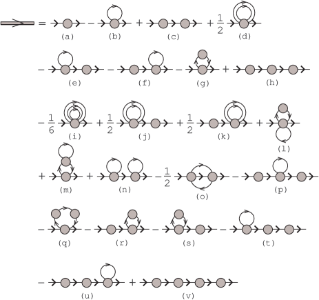
Figure 1: Diagrams of the first four orders of expansion (4).

All diagrams can be separated into two categories – those which can be divided into two parts by cutting some hopping line and those which cannot be divided in this way.Larkin ; Izyumov These latter diagrams are referred to as irreducible diagrams. In Fig. 1 the diagrams (c), (e), (f), (h), (j), (k), (n), (p), and (r)–(v) belong to the first category, while the others are from the second category. The former diagrams can be constructed from the irreducible diagrams by connecting them with hopping lines. Notice that a prefactor $\nu$ of some composite diagram is the product of prefactors of its irreducible parts [cf., e.g., the irreducible diagrams (a), (d) and the composed diagrams (j), (k) in Fig. 1]. If we denote the sum of all irreducible diagrams as $K({\bf n^{\prime}}\tau^{\prime},{\bf n}\tau)$, the equation for Green’s function can be written as

$$G({\bf n^{\prime}}\tau^{\prime},{\bf n}\tau) = K({\bf n^{\prime}}\tau^{\prime},{\bf n}\tau)+\sum_{{\bf n}_{1}{\bf n}^{\prime}_{1}}\int_{0}^{\beta}d\tau_{1}K({\bf n^{\prime}}\tau^{\prime},{\bf n}_{1}\tau_{1})$$ (6)

$$\times t_{{\bf n}_{1}{\bf n}^{\prime}_{1}}G({\bf n}^{\prime}_{1}\tau_{1},{\bf n}\tau).$$

This equation has the form of the Larkin equation. Larkin

The partial summation can be carried out in the hopping lines of cumulants by inserting the irreducible diagrams into these lines. In doing so the hopping constant $t_{\bf nn^{\prime}}$ in the respective formulas is substituted by

$$\Theta({\bf n\tau,n^{\prime}\tau^{\prime}}) = t_{\bf nn^{\prime}}\delta(\tau-\tau^{\prime})$$ (7)

$$+ \sum_{{\bf n}_{1}{\bf n}^{\prime}_{1}}t_{{\bf nn}^{\prime}_{1}}\int_{0}^{\beta}d\tau_{1}K({\bf n}^{\prime}_{1}\tau,{\bf n}_{1}\tau_{1})$$

$$\times \Theta({\bf n}_{1}\tau_{1},{\bf n}^{\prime}\tau^{\prime}).$$

For the diagram (b) in Fig. 1 inserting irreducible diagrams into the hopping line leads to the diagrams (g), (m), and (q).

Due to the translation and time invariance of the problem the quantities in Eqs. (6) and (7) depend only on differences of site indices and times. The use of the Fourier transformation

$$G({\bf k},i\omega_{l})=\sum_{\bf n^{\prime}}e^{i{\bf k(n^{\prime}-n)}}\int_{0}^{\beta}e^{i\omega_{l}(\tau^{\prime}-\tau)}G({\bf n}^{\prime}\tau^{\prime},{\bf n}\tau),$$

where $\omega_{l}=(2l+1)\pi T$ is the Matsubara frequency, simplifies significantly these equations:

$$G({\bf k},i\omega_{l}) = \frac{K({\bf k},i\omega_{l})}{1-t_{\bf k}K({\bf k},i\omega_{l})},$$ (8)

$$\Theta({\bf k},i\omega_{l}) = \frac{t_{\bf k}}{1-t_{\bf k}K({\bf k},i\omega_{l})}$$ (9)

$$= t_{\bf k}+t_{\bf k}^{2}G({\bf k},i\omega_{l}).$$

In the approximation used below the total collection of irreducible diagrams $K({\bf k},i\omega_{l})$ is substituted by the sum of the two simplest diagrams (a) and (b) appearing in the first two orders of the perturbation theory. Due to the form of the latter diagram this approximation is referred to as the one-loop approximation. In the diagram (b) the hopping line is renormalized in accordance with Eq. (9). Thus,

$$K(i\omega_{l}) = K_{1}(i\omega_{l})-T\sum_{l_{1}\sigma_{1}}K_{2}(i\omega_{l}\sigma,i\omega_{l_{1}}\sigma_{1},i\omega_{l_{1}}\sigma_{1})$$ (10)

$$\times \frac{1}{N}\sum_{\bf k}t^{2}_{\bf k}G({\bf k},i\omega_{l_{1}}),$$

where $K_{1}(i\omega_{l})$ and

$$K_{2}(i\omega_{l^{\prime}}\sigma,i\omega_{l}\sigma,i\omega_{l^{\prime}_{1}}\sigma_{1},i\omega_{l_{1}}\sigma_{1})$$

$$\quad=\int\!\!\!\!\int\!\!\!\!\int\!\!\!\!\int_{0}^{\beta}d\tau^{\prime}d\tau d\tau^{\prime}_{1}d\tau_{1}e^{-i\omega_{l^{\prime}}\tau^{\prime}+i\omega_{l}\tau-i\omega_{l^{\prime}_{1}}\tau^{\prime}_{1}+i\omega_{l_{1}}\tau_{1}}$$

$$\quad\quad\times K_{2}(\tau^{\prime}\sigma,\tau\sigma,\tau^{\prime}_{1}\sigma_{1},\tau_{1}\sigma_{1})$$

$$\quad=\beta\delta_{l+l_{1},l^{\prime}+l^{\prime}_{1}}K_{2}(i\omega_{l}\sigma,i\omega_{l^{\prime}_{1}}\sigma_{1},i\omega_{l_{1}}\sigma_{1})$$

are the Fourier transforms of cumulants (5), $N$ is the number of sites and we set $\sum_{\bf k}t_{\bf k}=0$. Notice that in this approximation $K$ does not depend on momentum.

Now we need to calculate the cumulants in Eq. (10). To do this it is convenient to introduce the Hubbard operators $X^{ij}_{\bf n}=|i{\bf n}\rangle\langle j{\bf n}|$ where $|i{\bf n}\rangle$ are eigenvectors of site Hamiltonians forming $H_{0}$, Eq. (LABEL:division). For each site there are four such states: the empty state $|0{\bf n}\rangle$ with the energy $E_{0}=0$, the two degenerate singly occupied states $|\sigma{\bf n}\rangle$ with the energy $E_{1}=-\mu$ and the doubly occupied state $|2{\bf n}\rangle$ with the energy $E_{2}=U-2\mu$. The Hubbard operators are connected by the relations

$$a_{\bf n\sigma}=X^{0\sigma}_{\bf n}+\sigma X^{-\sigma,2}_{\bf n},\quad a^{\dagger}_{\bf n\sigma}=X^{\sigma 0}_{\bf n}+\sigma X^{2,-\sigma}_{\bf n}$$ (11)

with the creation and annihilation operators. The commutation relations for the Hubbard operators are easily derived from their definition. Using Eq. (11) the first cumulant in Eq. (5) can be computed straightforwardly:

$$K_{1}(i\omega_{l})=\frac{1}{Z_{0}}\left(\frac{e^{-\beta E_{\sigma}}+e^{-\beta E_{0}}}{i\omega_{l}-E_{\sigma 0}}+\frac{e^{-\beta E_{2}}+e^{-\beta E_{\sigma}}}{i\omega_{l}-E_{2\sigma}}\right),$$ (12)

where $Z_{0}=e^{-\beta E_{0}}+2e^{-\beta E_{\sigma}}+e^{-\beta E_{2}}$ is the partition function, $E_{ij}=E_{i}-E_{j}$. As indicated in Refs. Izyumov, ; Vladimir, ; Pairault, , if $K({\bf k},i\omega_{l})$ is approximated by this cumulant the result corresponds to the Hubbard-I approximation. Hubbard63

To calculate $K_{2}$ it is convenient to use Wick’s theorem for Hubbard operators: Westwanski ; Stasyuk ; Zaitsev ; Izyumov

$$\langle{\cal T}X_{\alpha_{1}}(\tau_{1})\ldots X_{\alpha_{i}}(\tau_{i})X_{\alpha}(\tau)X_{\alpha_{i+1}}(\tau_{i+1})\ldots X_{\alpha_{n}}(\tau_{n})\rangle$$

$$\quad=\sum_{k=1}^{n}(-1)^{P_{k}}g_{\alpha}(\tau-\tau_{k})\langle{\cal T}X_{\alpha_{1}}(\tau_{1})\ldots$$

$$\quad\quad\times[X_{\alpha_{k}},X_{\alpha}]_{\pm}(\tau_{k})\ldots X_{\alpha_{n}}(\tau_{n})\rangle,$$ (13)

where the averaging and time dependencies of operators are determined by the Hamiltonian $H_{0}$, $\alpha$ is the index combining the state and site indices of the Hubbard operator. If $X_{\alpha}$ is a fermion operator ($X^{0\sigma}$, $X^{\sigma 2}$ and their conjugates), $P_{k}$ is the number of permutation with other fermion operators which is necessary to transfer the operator $X_{\alpha}$ from its position in the left-hand side of Eq. (13) to the position in the right-hand side. In this case

$$g_{\alpha}(\tau)=\frac{e^{E_{ij}\tau}}{e^{\beta E_{ij}}+1}\left\{\begin{array}[]{rl}-1,&\tau>0,\\ e^{\beta E_{ij}},&\tau<0,\end{array}\right.$$ (14)

where $i$ and $j$ are the state indices of $X_{\alpha}$. If $X_{\alpha}$ is a boson operator ($X^{00}$, $X^{22}$, $X^{\sigma\sigma^{\prime}}$, $X^{02}$, and $X^{20}$), $P_{k}=0$ and

$$g_{\alpha}(\tau)=\frac{e^{E_{ij}\tau}}{e^{\beta E_{ij}}-1}\left\{\begin{array}[]{rl}1,&\tau>0,\\ e^{\beta E_{ij}},&\tau<0.\end{array}\right.$$ (15)

In Eq. (13), $[X_{\alpha_{k}},X_{\alpha}]_{\pm}$ denotes an anticommutator when both operators are of fermion type and a commutator in other cases.

The substitution of Eq. (11) in $\langle{\cal T}\bar{a}_{\sigma}(\tau^{\prime})a_{\sigma}(\tau)\bar{a}_{\sigma_{1}}(\tau^{\prime}_{1})$ $\times a_{\sigma_{1}}(\tau_{1})\rangle$ in $K_{2}$, Eq. (5), leads to six nonvanishing averages of Hubbard operators (such averages are nonzero if the numbers of the operators $X^{0\sigma}$ and $X^{\sigma 0}$ coincide in them, and the same is true for the pair $X^{\sigma 2}$ and $X^{2\sigma}$). Applying Wick’s theorem (13) to these averages the number of operators in them is sequentially decreased until only time-independent operators are retained. For $H_{0}$ in Eq. (LABEL:division) these are $X^{00}$, $X^{\sigma\sigma^{\prime}}$, and $X^{22}$. Their averages are easily calculated. As a result, after some algebra we find

$$\sum_{\sigma_{1}}K_{2}(i\omega_{l}\sigma,i\omega_{l_{1}}\sigma_{1},\omega_{l_{1}}\sigma_{1})=-Z_{0}^{-1}U\bigl{\{}e^{-\beta E_{0}}g_{0\sigma}(i\omega_{l})$$

$$\quad\times g_{0\sigma}(i\omega_{l_{1}})g_{02}(i\omega_{l}+i\omega_{l_{1}})\bigl{[}g_{0\sigma}(i\omega_{l})+g_{0\sigma}(i\omega_{l_{1}})\bigr{]}$$

$$\quad+e^{-\beta E_{2}}g_{\sigma 2}(i\omega_{l})g_{\sigma 2}(i\omega_{l_{1}})g_{02}(i\omega_{l}+i\omega_{l_{1}})$$

$$\quad\times\bigl{[}g_{\sigma 2}(i\omega_{l})+g_{\sigma 2}(i\omega_{l_{1}})\bigr{]}+e^{-\beta E_{1}}\bigl{[}g_{0\sigma}(i\omega_{l})g_{\sigma 2}(i\omega_{l})$$

$$\quad\times\bigl{(}g_{0\sigma}(i\omega_{l_{1}})-g_{\sigma 2}(i\omega_{l_{1}})\bigr{)}^{2}+g_{0\sigma}(i\omega_{l_{1}})g_{\sigma 2}(i\omega_{l_{1}})$$

$$\quad\times\bigl{(}g_{0\sigma}^{2}(i\omega_{l})+g_{\sigma 2}^{2}(i\omega_{l})\bigr{)}\bigr{]}\bigr{\}}-Z_{0}^{-2}U^{2}\beta\delta_{ll_{1}}\bigl{(}e^{-\beta(E_{0}+E_{2})}$$

$$\quad+2e^{-\beta(E_{0}+E_{1})}+3e^{-2\beta E_{1}}+2e^{-\beta(E_{1}+E_{2})}\bigr{)}g_{0\sigma}^{2}(i\omega_{l})$$

$$\quad\times g_{\sigma 2}^{2}(i\omega_{l})+Z_{0}^{-2}U^{2}\beta\bigl{(}2e^{-\beta(E_{0}+E_{2})}+e^{-\beta(E_{0}+E_{1})}$$

$$\quad+e^{-\beta(E_{1}+E_{2})}\bigr{)}g_{0\sigma}(i\omega_{l})g_{\sigma 2}(i\omega_{l})g_{0\sigma}(i\omega_{l_{1}})g_{\sigma 2}(i\omega_{l_{1}}),$$

(16)

where $g_{ij}(i\omega_{l})=(i\omega_{l}+E_{ij})^{-1}$ is the Fourier transform of functions (14) and (15).

In this work the case of half-filling is considered. In this case $\mu=\frac{U}{2}$ and cumulants (12) and (16) are significantly simplified if we additionally suppose that $T\ll U$:

$$K_{1}(i\omega_{l})=\frac{i\omega_{l}}{(i\omega_{l})^{2}-\bigl{(}\frac{U}{2}\bigr{)}^{2}},$$

$$\sum_{\sigma_{1}}K_{2}(i\omega_{l}\sigma,i\omega_{l_{1}}\sigma_{1},\omega_{l_{1}}\sigma_{1})$$

$$\quad=-\frac{U}{2}\Biggl{(}\frac{U^{2}}{\bigl{[}(i\omega_{l})^{2}-\bigl{(}\frac{U}{2}\bigr{)}^{2}\bigr{]}\bigl{[}(i\omega_{l_{1}})^{2}-\bigl{(}\frac{U}{2}\bigr{)}^{2}\bigr{]}^{2}}$$ (17)

$$\quad\quad+\frac{2[(i\omega_{l})^{2}+\bigl{(}\frac{U}{2}\bigr{)}^{2}]}{\bigl{[}(i\omega_{l})^{2}-\bigl{(}\frac{U}{2}\bigr{)}^{2}\bigr{]}^{2}\bigl{[}(i\omega_{l_{1}})^{2}-\bigl{(}\frac{U}{2}\bigr{)}^{2}\bigr{]}}\Biggr{)}$$

$$\quad\quad-\beta\delta_{ll_{1}}\frac{3\bigl{(}\frac{U}{2}\bigr{)}^{2}}{(i\omega_{l})^{2}-\bigl{(}\frac{U}{2}\bigr{)}^{2}}.$$

The first term in the equation for $\sum_{\sigma_{1}}K_{2}$ is the even function of $i\omega_{l_{1}}$. It does not contribute to the sum over $l_{1}$ in Eq. (10), since $\sum_{\bf k}t^{2}_{\bf k}G({\bf k},i\omega_{l_{1}})$ is supposed to be an odd function of $i\omega_{l_{1}}$. Thus, finally Eq. (10) acquires the form

$$K(i\omega_{l}) = \frac{i\omega_{l}}{(i\omega_{l})^{2}-\bigl{(}\frac{U}{2}\bigr{)}^{2}},$$ (18)

$$+ \frac{3\bigl{(}\frac{U}{2}\bigr{)}^{2}}{\bigl{[}(i\omega_{l})^{2}-\bigl{(}\frac{U}{2}\bigr{)}^{2}\bigr{]}^{2}}\frac{1}{N}\sum_{\bf k}t^{2}_{\bf k}G({\bf k},i\omega_{l_{1}}).$$

Analogous equations were obtained in Refs. Izyumov, ; Vladimir, ; Pairault, (in Ref. Izyumov, the last term in the right-hand side of the equation is three times smaller, because diagrams with spin propagators were not taken into account there).

Let us turn to real frequencies by substituting $i\omega_{l}$ with $z=\omega+i\eta$ where $\eta$ is a small positive constant which affords an artificial broadening. Results given in the next section were calculated with $G({\bf k},z)$ in the right-hand side of Eq. (18) taken from the Hubbard-I approximation. As mentioned, this Green’s function is obtained if $K({\bf k}\omega)$ in Eq. (8) is approximated by the first cumulant (12). For half-filling we find

$$G({\bf k},z)=\frac{1}{2}\left(1+\frac{t_{\bf k}}{\sqrt{U^{2}+t_{\bf k}^{2}}}\right)\frac{1}{z-\varepsilon_{1,\bf k}}$$

$$\quad+\frac{1}{2}\left(1-\frac{t_{\bf k}}{\sqrt{U^{2}+t_{\bf k}^{2}}}\right)\frac{1}{z-\varepsilon_{2,\bf k}},$$

(19)

$$\varepsilon_{1,\bf k}=\frac{1}{2}\left(t_{\bf k}+\sqrt{U^{2}+t_{\bf k}^{2}}\right),$$

$$\varepsilon_{2,\bf k}=\frac{1}{2}\left(t_{\bf k}-\sqrt{U^{2}+t_{\bf k}^{2}}\right).$$

Below the two-dimensional square lattice is considered. It is supposed that only the hopping constants between nearest neighbor sites $t$ are nonzero which gives $t_{\bf k}=2t[\cos(k_{x})+\cos(k_{y})]$ where the intersite distance is taken as the unit of length.

III Spectral function

Figure 2 demonstrates $\Im K(\omega)$ calculated with the use of Eqs. (18) and (19). The change to real frequencies carried out in the previous section converts the Matsubara function (2) into the retarded Green’s function. Abrikosov It is an analytic function in the upper half-plane which requires that $\Im K(\omega)$ be negative. As seen from Fig. 2, this condition is violated at $\omega=\pm\frac{U}{2}$. This difficulty of the considered approximation was indicated in Ref. Pairault, . The problem is connected with divergencies at $\omega_{d}=\mu$ and $\mu-U$ introduced by functions $g_{0\sigma}(\omega)$ and $g_{\sigma 2}(\omega)$ in the above formulas. As can be seen from the procedure of calculating the cumulants in the previous section, these functions and divergencies with sign-changing residues will appear in all orders of the perturbation expansion (4). It can be expected that in the entire series the divergencies compensate each other, however, in the considered subset of terms such compensation does not occur. Nevertheless, as seen from Fig. 2, at frequencies neighboring to $\omega_{d}$ cumulants are regular and, if the used subset of diagrams is expected to give a correct estimate of the entire series for these frequencies, the value of $\Im K(\omega)$ at the singular frequencies can be reconstructed using an interpolation and its values in the regular region. An example of such interpolation is given in Fig. 2.

Figure 2: The imaginary part of $K(\omega)$ calculated using Eqs. (18) and (19) for a 100$\times$100 lattice, $t=-\frac{1}{8}U$ and $\eta=0.01U$ (the dashed line). The solid line shows the corrected $\Im K(\omega)$ (see text).

The function $K(z)$ has to be analytic in the upper half-plane also and therefore its real part can be calculated from its imaginary part using the Kramers-Kronig relations. We use this way with the interpolated $\Im K(\omega)$ to avoid the influence of the divergencies on $\Re K(\omega)$. However, the use of the interpolation overrates somewhat values of $|\Im K(\omega)|$ which leads to the overestimation of the tails in the real part. To correct this defect the interpolated $K(\omega)$ is scaled so that its real part for frequencies $|\omega|\gg\frac{U}{2}$ coincide with the values obtained from Eq. (18). It is worth noting that such obtained spectral function

$$A({\bf k}\omega) = -\frac{1}{\pi}\Im G({\bf k}\omega)$$ (20)

$$= -\frac{1}{\pi}\frac{\Im K(\omega)}{[1-t_{\bf k}\Re K(\omega)]^{2}+[t_{\bf k}\Im K(\omega)]^{2}}$$

satisfies the normalization condition $\int_{-\infty}^{\infty}d\omega A({\bf k}\omega)=1$ with an accuracy better than 0.01.

Figure 3: The spectral function $A({\bf k}\omega)$ calculated for momenta along the route shown in the inset. An 8$\times$8 lattice, $t=-\frac{1}{4}U$ and $\eta=0.2U$.

The spectral function obtained in this way with the use of Eqs. (18), (19), and (20) for momenta in the Brillouin zone of an 8$\times$8 lattice is shown in Fig. 3. In these calculations the small lattice and a comparatively large artificial broadening were used to reproduce the conditions of Monte-Carlo calculations carried out in Ref. Moukouri, . Comparing Fig. 3 with Fig. 5 in that work we find close similarity of these two groups of spectra – not only the general shapes of spectra are close but also the position of maxima in them. Some discrepancies can be also noticed. In particular, in the spectrum for ${\bf k}=(\frac{\pi}{2},\frac{\pi}{4})$ in Fig. 3 the intensity of maximum at a positive frequency is larger than in the respective spectrum in Ref. Moukouri, (in this latter spectrum this maximum looks like a barely perceptible peculiarity).

The spectral function for a larger $U$ is shown in Fig. 4 where the momenta along the symmetry lines of the square Brillouin zone were chosen. Let us compare these results with the spectra in Fig. 1 in Ref. Grober, which were obtained in Monte-Carlo calculations with the same ratio $U/|t|$ in an 8$\times$8 lattice. We found that the results shown in Fig. 4 change only slightly with decreasing the lattice size to this value. The comparison has to be carried out with low-temperature spectra of Ref. Grober, , since Eq. (17) used in our calculations was derived for the case $T\ll U$. Notice that in this limit at half-filling the spectral function in the used approximation does not depend on temperature. Again we find that our calculated spectra are close to those obtained in the Monte-Carlo calculations, though there are some differences in relative intensity of maxima. In our spectra some maxima resolved in the Monte-Carlo calculations look like shoulders of main maxima and a decrease of the artificial broadening $\eta$ does not convert the shoulders to maxima. On the other hand, the maxima at $\omega\approx 2|t|$ in the spectra for momenta near $(0,0)$ and at $\omega\approx-2|t|$ in the spectra for momenta near $(\pi,\pi)$ which are well resolved in our results are barely perceptible in Fig. 1 of Ref. Grober, . The possible reason for these differences can be established from the comparison of Figs. 3 and 4. The respective maxima in the former figure for the smaller $U$ are less intensive. Apparently, like the Hubbard-I approximation, the used approach somewhat overestimates the electron correlations. Nevertheless, Fig. 4 reproduces correctly the most essential features of the spectra obtained by the Monte-Carlo method.

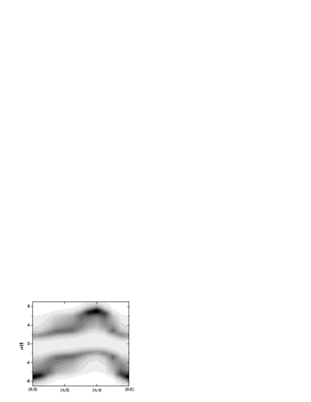
Figure 4: The upper panel: the spectral function $A({\bf k}\omega)$ calculated for momenta along the symmetry lines of the square Brillouin zone. The lower panel: the dispersion of maxima in the upper panel shown as a gray-scale plot with darker areas corresponding to larger intensity of maxima. A 100$\times$100 lattice, $t=-\frac{1}{8}U$ and $\eta=0.1U$.

One of these features recently reproduced also in the cluster perturbation Dahnken and the two-particle self-consistent Tremblay calculations is the four-band structure of the spectrum. In Fig. 4 these bands are located near frequencies $\omega=\pm 3|t|$ and $\omega=\pm 6|t|$. The high-frequency bands are observed near the $(0,0)$ and $(\pi,\pi)$ points, while the low-frequency bands have a larger existence domain in our calculations. Similar four bands can be identifies in Fig. 3. A more detailed treatment of the low-frequency bands shows that either of them in turn contain two components. Maxima in $A({\bf k}\omega)$ arise by two reasons – due to the smallness of the denominator in Eq. (20) when a frequency satisfying the equation $1-t_{\bf k}\Re K(\omega)=0$ falls into a region of a small damping $|\Im K(\omega)|$ and due to the strong frequency dependence of $\Im K(\omega)$ in the numerator of Eq. (20). The high-frequency bands and the low-frequency bands in the central part and at the periphery of the Brillouin zone arise due to the first reason. As seen from Fig. 2, the regions of small damping are located on either side of the two maxima in $\Im K(\omega)$ which gives rise to the well-separated four bands. However, for momenta which are close to the boundary of the magnetic Brillouin zone the equation $1-t_{\bf k}\Re K(\omega)=0$ has no solutions due to a small or vanishing $t_{\bf k}$. In this case the two maxima of $A({\bf k}\omega)$ originate from the two maxima in $|\Im K(\omega)|$. They are located in the same frequency ranges as the low-frequency maxima originated from the resonance denominator in Eq. (20). Therefore they can be combined in a common dispersion band, although widths of the maxima of different origin can significantly vary for a smaller artificial broadening.

As can be seen from Eqs. (8), (18), and (19), the used approximation does not describe the Mott transition – for $\eta\rightarrow 0$ the density of states $\rho(\omega)=N^{-1}\sum_{\bf k}A({\bf k}\omega)$ at $\omega=0$ vanishes for any finite $U$. This flaw can be remedied by going to the next approximation. The use of approximation (19) in Eq. (18) means that only diagrams (a) in Fig. 1 are inserted in the hopping line of the diagram (b). If these latter diagrams are also inserted in the line, Eq. (18) is transformed to the following self-consistent equation for the irreducible part:

$$K(z) = \frac{z}{z^{2}-\bigl{(}\frac{U}{2}\bigr{)}^{2}},$$ (21)

$$+ \frac{3\bigl{(}\frac{U}{2}\bigr{)}^{2}}{\bigl{[}z^{2}-\bigl{(}\frac{U}{2}\bigr{)}^{2}\bigr{]}^{2}}\frac{1}{N}\sum_{\bf k}\frac{t_{\bf k}}{1-t_{\bf k}K(z)}.$$

For the initial electron dispersion $t_{\bf k}$ described by the semielliptical density of states

$$\rho_{0}(\omega)=\left\{\begin{array}[]{rl}\frac{2}{\pi B}\sqrt{1-\left(\frac{\omega}{B}\right)^{2}},&|\omega|\leq B,\\ 0,&|\omega|>B,\end{array}\right.$$

where $B$ is the halfwidth of the band, Eq. (21) can be solved analytically and the condition for the disappearance of the gap at $\omega=0$ in $\rho(\omega)$ can be found. It happens when $U\leq U_{c}=\sqrt{3}B$ and the gap opens when $U>U_{c}$. Analogous results for somewhat different equations and initial dispersions were obtained in Refs. Zaitsev, ; Izyumov, ; Pairault, .

IV Conclusion

The considered diagram technique is very promising for a generalization to many-band Hubbard models for which energy parameters of the one-site parts of the Hamiltonians exceed or at least are comparable to the intersite parameters. The expansion in powers of these latter parameters can be expressed in terms of cumulants in the same manner as discussed above. Now there are distinct cumulants which belong to different site states characterized by dissimilar parameters of the repulsion and the level energy. These cumulants are described by formulas similar to Eqs. (12) and (16). For example, for the Emery model Emery which describes oxygen $2p_{\sigma}$ and copper $3d_{x^{2}-y^{2}}$ orbitals of Cu-O planes in high-$T_{c}$ superconductors there are two types of cumulants corresponding to these states. Diagrams of the lowest orders, e.g., for Green’s function on copper sites resemble those shown in Fig. 1 where “oxygen” cumulants are included in hopping lines. Equations of the type of Eq. (8) and partial summations similar to Eq. (9) can be derived also in this case.

In summary, the diagram technique for the one-band Hubbard model was formulated for the case of moderate to strong Hubbard repulsion. The expansion in powers of the hopping constant is expressed in terms of site cumulants of electron creation and annihilation operators. For Green’s function the equation of the Larkin type was derived and solved for the case of two dimensions, nearest-neighbor hopping and half-filling. The obtained spectrum contains four bands. It was shown that maxima of the spectral function forming the bands are of dissimilar origin in different regions of the Brillouin zone – in its central part and at the periphery the maxima stem from the resonance denominator in the formula for the spectral function, while near the boundary of the magnetic Brillouin zone they originate from the strong frequency dependence of the irreducible part in the numerator of this formula. The obtained band structure and the shapes of the spectral function are close to those found in the Monte Carlo calculations.

- (1) M. C. Gutzwiller, Phys. Rev. Lett. 10, 159 (1963).
- (2) J. Hubbard, Proc. R. Soc. London, Ser. A 276, 238 (1963).
- (3) J. Kanamori, Prog. Theor. Phys. 30, 275 (1963).
- (4) J. Hubbard, Proc. R. Soc. London, Ser. A 296, 82 (1966).
- (5) B. Westwanski and A. Pawlikovski, Phys. Lett. A 43, 201 (1973).
- (6) P. M. Slobodyan and I. V. Stasyuk, Teor. Mat. Fiz. 19, 423 (1974) [Theor. Mat. Phys. 19, 616 (1974)].
- (7) R. O. Zaitsev, ZhETF 70, 1100 (1976) [Sov. Phys. JETP 43, 574 (1976)].
- (8) Yu. A. Izyumov and Yu. N. Skryabin, Statistical Mechanics of Magnetically Ordered Systems, (Consultants Bureau, New York 1988).
- (9) S. G. Ovchinnikov and V. V. Valkov, Hubbard operators in the theory of strongly correlated electrons, (Imperial College Press, London, 2004).
- (10) M. I. Vladimir and V. A. Moskalenko, Teor. Mat. Fiz. 82, 428 (1990) [Theor. Mat. Phys. 82, 301 (1990)]; S. I. Vakaru, M. I. Vladimir and V. A. Moskalenko, Teor. Mat. Fiz. 85, 248 (1990) [Theor. Mat. Phys. 85, 1185 (1990)].
- (11) W. Metzner, Phys. Rev. B 43, 8549 (1991).
- (12) V. A. Moskalenko, P. Entel and D. F. Digor, Phys. Rev. B 59, 619 (1999).
- (13) S. Pairault, D. Sénéchal and A.-M. S. Tremblay, Eur. Phys. J. B 16, 85 (2000).
- (14) A. I. Larkin, ZhETF 37, 264 (1959) [Sov. Phys. JETP 37, 186 (1960)].
- (15) A. Moreo, S. Haas, A. W. Sandvik, and E. Dagotto, Phys. Rev. B 51, 12045 (1995).
- (16) R. Preuss, W. Hanke, and W. von der Linden, Phys. Rev. Lett. 75, 1344 (1995).
- (17) C. Gröber, R. Eder, and W. Hanke, Phys. Rev. B 62, 4336 (2000).
- (18) C. Dahnken, M. Aichhorn, W. Hanke, and M. Potthoff, Phys. Rev. B 70, 245110 (2004).
- (19) A.-M. S. Tremblay, B. Kyung, and D. Sénéchal, cond-mat/0511334 (unpublished).
- (20) A. A. Abrikosov, L. P. Gor’kov, and I. E. Dzyaloshinskii, Methods of Quantum Field Theory in Statistical Physics, (Pergamon Press, New York, 1965).
- (21) R. Kubo, J. Phys. Soc. Jpn. 17,1100 (1962).
- (22) S. Moukouri, S. Allen, F. Lemay, B. Kyung, D. Poulin, Y. M. Vilk, and A.-M. S. Tremblay, Phys. Rev. B 61, 7887 (2000).
- (23) V. J. Emery, Phys. Rev. Lett. 58, 2794 (1987).