Heat conduction in a confined solid strip: Response to external strain

Abstract

We study heat conduction in a system of hard disks confined to a narrow two dimensional channel. The system is initially in a high density solid-like phase. We study, through nonequilibrium molecular dynamics simulations, the dependence of the heat current on an externally applied elongational strain. The strain leads to deformation and failure of the solid and we find that the changes in internal structure can lead to very sharp changes in the heat current. A simple free-volume type calculation of the heat current in a finite hard-disk system is proposed. This reproduces some qualitative features of the current-strain graph for small strains.

I Introduction

In a recent study myfail it was observed that the properties of a solid that is confined in a narrow channel can change drastically for small changes in applied external strain. This was related to structural changes at the microscopic level such as a change in the number of layers of atoms in the confining direction. These effects occur basically as a result of the small ( few atomic layers in one direction ) dimensions of the system considered and confinement along some direction. A similar layering transition, in which the number of smectic layers in a confined liquid changes in discrete steps with increase in the wall-to-wall separation, was noted in degennes ; landman . Both myfail ; degennes look at equilibrium properties while landman looks at changes in the dynamical properties. An interesting question is, how are transport properties, such as electrical and thermal conductivity, affected for these nanoscale systems under strain? This question is also important to address in view of the current interest in the properties of nanosystems, both from the point of view of fundamentals and applications datta ; nanobook1 ; nanobook2 .

In this paper we consider the effect of strain on the heat current across a two-dimensional (2D) “solid” formed by a few layers of interacting atoms confined in a long narrow channel. We note here that, in the thermodynamic limit it is expected that there can be no true solid phase in this quasi-one-dimensional system. However for a long but finite channel, which is our interest here, and at a high packing fraction the fluctuations are small and the system behaves like a solid. We will use the word “solid” in this sense.

In Ref. myfail the anomalous failure, under strain, of a narrow strip of a 2D solid formed by hard disks confined within hard walls [ see Fig. 1 ] was studied. Sharp jumps in the stress vs strain plots were observed. These were related to structural changes in the system which underwent transitions from solid-to-smectic-to-modulated liquid phases myfail ; myijp . In the present paper we study changes in the thermal conductance of this system as it undergoes elastic deformation and failure through a layering transition caused by external elongational strains applied in different directions.

The calculation of heat conductivity in a many body system is a difficult problem. The Kubo formula and Boltzmann kinetic theory provide formal expressions for the thermal conductivity. In practice these are usually difficult to evaluate without making drastic approximations. More importantly a large number of recent studies bonet ; lepri ; lippi ; grass indicate that the heat conductivity of low-dimensional systems infact diverge. It is then more sensible to calculate directly the heat current or the conductance of the system rather than the heat conductivity. In this paper we propose a simple-minded calculation of the heat current which can be expected to be good for a hard disk (or hard spheres in the three dimensional case) system in the solid phase. This reproduces some qualitative features of the simulations and gives values for the current which are of the correct order of magnitude.

The organization of the paper is as follows. In Sec. (II) we explain the model and present the results from simulations. In Sec. (III) we derive a simple formula for heat current in a hard-sphere system and evaluate it approximately. We conclude with some discussions in Sec. (IV).

II Results from simulations

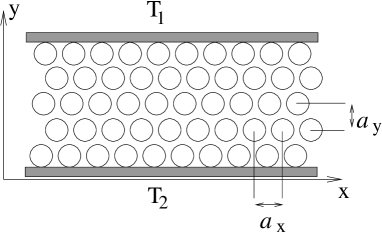
Figure 1: A solid with a triangular lattice structure formed by hard disks confined between two structureless walls at $y=0$ and $y=L_{y}$. The walls are maintained at two different temperatures. The lattice parameters of the unstrained solid are denoted by $a_{x}^{0}$ and $a_{y}^{0}$. Elongational strains can be imposed by rescaling distances either in the $x$ or $y$ directions and the lattice parameters change to $a_{x}$ and $a_{y}$.

We consider a 2D system of hard disks of diameter $d$ and mass $m$ which interact with each other through elastic collisions. The particles are confined within a narrow hard structureless channel [see Fig. 1]. The hard walls of the channel are located at $y=0$ and $y=L_{y}$ and we take periodic boundary conditions in the $x-$direction. The length of the channel along the $x-$direction is $L_{x}$ and the area is ${\cal A}=L_{x}\times L_{y}$. The confining walls are maintained at two different temperatures ( $T_{2}$ at $y=0$ and $T_{1}$ at $y=L_{y}$ ) so that the temperature difference $\Delta T=T_{2}-T_{1}$ gives rise to a heat current in the $y$-direction. Initially we start with channel dimensions $L_{x}^{0}$ and $L_{y}^{0}$ such that the system is in a phase corresponding to a unstrained solid with a triangular lattice structure. We then study the heat current in this system when it is strained (a) along the $x-$direction and (b) along the $y-$direction.

We perform an event-driven collision time dynamics allen simulation of the hard disk system. The upper and lower walls are maintained at temperatures $T_{1}=1$ and $T_{2}=2$ (in arbitrary units) respectively by imposing Maxwell boundary condition bonet at the two confining walls. This means that whenever a hard disk collides with either the lower or the upper wall it gets reflected back into the system with a velocity chosen from the distribution

$$f({\bf u})=\frac{1}{\sqrt{2\pi}}\left(\frac{m}{k_{B}T_{W}}\right)^{3/2}|u_{y}|\exp\left(-\frac{m{\bf u}^{2}}{2k_{B}T_{W}}\right)$$ (1)

where $T_{W}$ is the temperature ($T_{1}$ or $T_{2}$) of the wall on which the collision occurs. During each collision energy is exchanged between the system and the bath. Thus in our molecular dynamics simulation, the average heat current flowing through the system can be found easily by computing the net heat loss from the system to the two baths (say $Q_{1}$ and $Q_{2}$ respectively) during a large time interval $\tau$. The steady state heat current from lower to upper bath is given by $\langle I\rangle=\lim_{\tau\to\infty}Q_{1}/\tau=-\lim_{\tau\to\infty}Q_{2}/\tau$. In the steady state the heat current (the heat flux density integrated over $x$) is independent of $y$. This is a requirement coming from current conservation. However if the system has inhomogeneities then the flux density itself can have a spatial dependence and in general we can have $j=j(x,y)$. In our simulations we have also looked at $j(x,0)$ and $j(x,L_{y})$.

Note that the relevant scales in the problem are: $k_{B}T$ for energy, $d$ for length and $\tau_{s}=\sqrt{md^{2}/k_{B}T}$ for time. We start from a solid commensurate with its wall to wall separation and follow two different straining protocols. In case (a) we strain the solid by rescaling the length in the $x$-direction and the imposed external strain is $\epsilon_{xx}=(L_{x}-L_{x}^{0})/L_{x}^{0}$. In case (b) we rescale the length along the $y$-direction and the imposed strain is $\epsilon_{yy}=(L_{y}-L_{y}^{0})/L_{y}^{0}$.

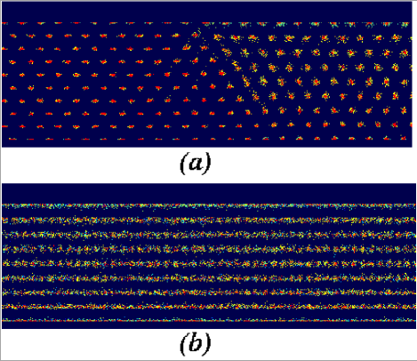
Figure 2: (Color online) Plots obtained by superposition of $500$ steady state configurations of a portion of $40\times 10$ system taken at equal time intervals. Starting from $\eta=0.85$ imposition of strains (a) $\epsilon_{xx}=0.1$, (b) $\epsilon_{xx}=0.15$ gives rise to these structures. The colors code local density of points from red/dark (high) to blue/light (low). In (a) one can see a $9$-layered structure nucleated within a $10$-layered solid. The corresponding structure factor identifies this to be a smectic myfail . In (b) the whole system has transformed into a $9$-layered smectic.

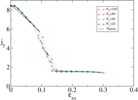
Figure 3: (Color online) Plot of $j_{y}$ vs $\epsilon_{xx}$ for different lengths of the channel. In this graph as well as in all other view graphs we plot $j_{y}$ in units of $k_{B}T/\tau_{s}d$. The width of the channel is $N_{y}=10$ layers. Starting packing fraction is $\eta=0.85$. The solid line shows the theoretical prediction of dependence of the heat current on strain [see Sec. (III)].

The only thermodynamically relevant variable for a hard disk system is the packing fraction $\eta=\pi Nd^{2}/4{\cal A}$. For a close packed solid with periodic boundary condition this value is about $\eta_{c}=0.9069$. On the other hand for a confined solid having $N_{y}$ number of layers $\eta_{c}=\pi N_{y}/(2\sqrt{3}(N_{y}-1)+4)$ and for a $10$- layered solid $\eta_{c}=0.893$. In our simulations we consider initial values of $\eta$ for the solid to be close to $\eta_{c}$. The channel is “mesoscopic” in the sense that it has a small width with $N_{y}=10$ layers of disks in the $y-$direction (in the initially unstrained solid). In the $x-$direction the system can be big and we consider $N_{x}=20,~{}40,~{}80,~{}160$ number of disks in the $x-$direction. In collision time dynamics we perform $10^{5}$ collisions per particle to reach the steady state and collect data over another $10^{5}$ collisions per particle. All the currents calculated in this study are accurate within error bars which are less than $3\%$ of the average current.

Let us briefly mention some of the equilibrium results for the stress-strain behavior obtained in Ref. myfail . As the strain $\epsilon_{xx}$ is imposed, the perfectly triangular solid shows rectangular distortion along with a linear response in strain vs stress behavior. Above a critical strain ($\epsilon_{xx}\approx 0.1$) one finds that smectic bands having a lesser number of layer nucleate within the solid [this can also be seen in Fig. (2a) obtained from a nonequilibrium simulation]. This smectic is liquid-like in the $x$-direction (parallel to the walls) and has solid-like density modulation order in the $y$-direction (perpendicular to the walls). With further increase in strain, the size of the smectic region increases and ultimately the whole system goes over to the smectic phase at $\epsilon_{xx}\approx 0.15$ [Fig. (2b)]. At even higher strains the smectic melts to a modulated liquid myfail ; myijp . The corresponding structure factor shows typical liquid like ring pattern superimposed with smectic like density modulation peaks. This layering transition is an effect of finite size in the confining direction. Similar phase behavior has been observed in experiments on steel balls confined in quasi 1D pieranski-1 . We note that, to fit a $N_{y}$ layered triangular solid within a channel of width $L_{y}$ we require

$$L_{y}=\frac{\sqrt{3}}{2}a_{x}^{0}(N_{y}-1)+d~{}.$$ (2)

This enables us to define a fictitious number of layers

$$\chi=2\frac{L_{y}-d}{\sqrt{3}a}+1$$

of triangular solid that can span the channel where $a$ is the lattice parameter at any given density. The actual number of layers that are present in the strained solid is $N_{y}=I(\chi)$ where the function $I(\chi)$ gives the integer part of $\chi$. For confined solids the free energy has minima at integer values of $\chi$ and maxima at half-integral values myijp ; myfail . The difference in free-energy between successive maxima and minima gradually decreases with increasing $L_{y}$. Thereby the layering transition washes out for $n_{l}\gtrsim 25$ layered unstrained solidmyfail . Up to this number of layers, a triangular solid strip confined between two planar walls fails at a critical deviatoric strain $\epsilon^{\ast}_{d}\sim 1/N_{y}$ (where $\epsilon_{d}=\epsilon_{xx}-\epsilon_{yy}$). Smaller strips fail at a larger deviatoric strain.

We now present the heat conduction simulation results for the two cases of straining in $x$ and $y$ directions.

(a) Strain in $x$-direction -  In Fig. 3 we plot the heat current density $j_{y}$ calculated at different values of the strain $\epsilon_{xx}$. Starting from the triangular lattice configuration, we find that the heat current decreases linearly with increase in strain. At about the critical strain $\epsilon_{xx}\approx 0.1$ we find that the heat current begins to fall at a faster rate. This is easy to understand physically. At the onset of critical strain, smectic bands, which have lesser number of particle layers, start nucleating (Fig. 2). These regions are much less effective in transmitting heat than the solid phase and the heat current falls rapidly as the size of the smectic bands grow. At about the strain value $\epsilon_{xx}\approx 0.15$ the whole system is spanned by the smectic. Beyond this strain there is no appreciable change in the heat current. The solid line in Fig. 3 is an estimate from a simple analysis explained in Sec. (III).

In Fig. 4 we plot the local steady state heat current $j_{y}(x)$ for a system of $40\times 10$ particles at a strain $\epsilon_{xx}=0.118$ i.e. at a strain corresponding to the solid-smectic phase coexistence. At this same strain the number of layers averaged over $10^{3}$ configurations have been plotted. It clearly shows that the local heat current is smaller in regions with smaller number of layers. This is the reason behind getting a sharp drop in average heat current after the onset of phase coexistence.

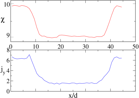
Figure 4: (Color online) $\chi(x)$ is the local number of layers averaged over $10^{3}$ steady state configurations for a system of $40\times 10$ hard disks. A starting triangular lattice of $\eta=0.85$ is strained to $\epsilon_{xx}=0.118$ and the data collected after steady state reached. Also shown is the local heat current $j_{y}(x)$. The regions having lower number of layers conduct less effectively.

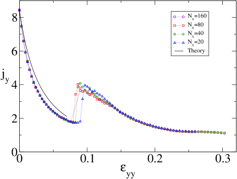
Figure 5: (Color online) Plot of $j_{y}$ vs $\epsilon_{yy}$ for different channel lengths. The channel width is $N_{y}=10$ layers. The starting packing fraction is $\eta=0.85$. The jump in current occurs at the strain value where the number of layers in the $y-$direction increases by one and the system goes to a smectic phase. The solid line shows the theoretical prediction of dependence of the heat current on strain [ see Sec. (III) ].

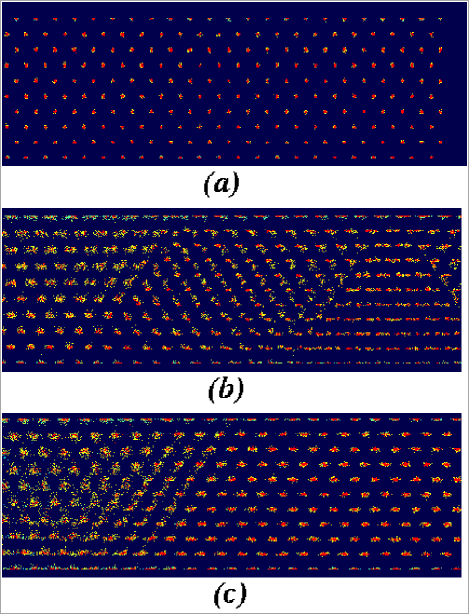
Figure 6: (Color online) Plots obtained by superposition of $500$ steady state configurations of a portion of $40\times 10$ system taken at equal time intervals. Starting from $\eta=0.85$ imposition of strains (a) $\epsilon_{yy}=0.05$, (b) $\epsilon_{yy}=0.1$, (c) $\epsilon_{yy}=0.12$ gives rise to these structures. The colors code local density of points from red/dark (high) to blue/light (low). (a) Solid phase. (b) A mixture of $10$-layered solid and a buckling phase. (c) An $11$-layered solid in contact with $10$-layered smectic like region.

(b)Strain in $y$-direction -  Next we consider the case where, again starting from the density $\eta=0.85$, we impose a strain along the $y-$direction. As shown in Fig. 5, the heat current $j_{y}$ now has a completely different nature. The initial fall is much steeper and has a form different from the linear drop in Fig. 3. The approximate analytic curve is explained in Sec. (III). At about $\epsilon_{yy}\approx 0.1$ we see a sharp and presumably discontinuous jump in the current. At this point the system goes over to a buckled phase (Fig. 6b) in which different parts of the solid (along $x$-direction) are displaced along the $y$-direction by small amounts so that the extra space between the walls is covered buckled-1 ; buckled-2 ; buckled-3 . A further small strain induces a layering transition and the system breaks into two regions one of which is an $N_{y}=11$ layered solid and the other is a $N_{y}=10$ layered highly fluctuating smectic-like region. At even higher strains ($\epsilon_{yy}\sim 0.2$) the whole system eventually melts to an $N_{y}=11$ layered smectic phase. The phase behavior of this system is interesting and will be discussed in detail elsewheremyfail-large . Unlike the case where the applied strain is in the $x$-direction, in the present case the buckling-layering transition is very sharp. Even though the overall density has decreased, due to buckling and increase in number of layers in the conducting direction, there is an increase in the energy transferring collisions and hence the heat current. The plots in Fig. 6 show the structural changes that occur in the system as one goes through the transition.

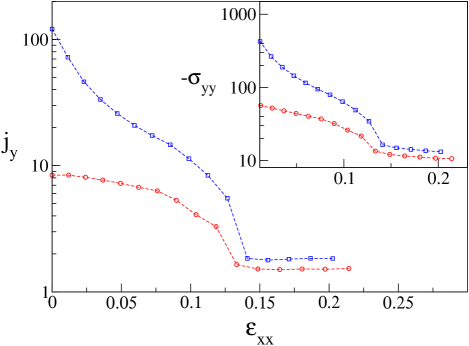
Figure 7: (Color online) Plot of $j_{y}$ vs $\epsilon_{xx}$ for two different starting values of the packing fraction. $\Diamond$ corresponds to a starting value of $\eta=0.89$ while $+$ is for $\eta=0.85$. In both the cases the initial solid size was $80\times 10$. The inset shows corresponding plots of $-\sigma_{yy}$ (in units of $k_{B}T/d^{2}$) vs $\epsilon_{xx}$. Notice that stress-strain curve has the same qualitative profile as the $j_{y}$ vs $\epsilon_{xx}$ curve.

We find in general that the heat current along any direction within the solid shows the same qualitative features as the stress component along the same direction. This can be seen in Fig.7 where we have plotted $j_{y}$ vs $\epsilon_{xx}$ for two starting densities of solids $\eta=0.85,~{}0.89$. In the inset we show the corresponding $-\sigma_{yy}$ vs $\epsilon_{xx}$ curves and see that they follow the same qualitative behavior as the heat current curves. The reason for this is that microscopically they both originate from interparticle collisions. Infact the microscopic expressions for the total heat current [ see Eq. (11) in Sec. (III) ] is very similar to that for the stress tensor component, with an extra velocity factor. The stress tensor is given by:

$${\cal A}\sigma_{\alpha\beta} = -\sum_{i}\langle mu_{i}^{\alpha}u_{i}^{\beta}\rangle+\sum_{i<j}\left\langle\frac{\partial\phi(r_{ij})}{\partial r_{ij}}\frac{x_{ij}^{\alpha}x_{ij}^{\beta}}{r_{ij}}\right\rangle~{},$$ (3)

where $\{x_{i}^{\alpha},u_{i}^{\alpha}\}$ refer to the $\alpha$-th component of position and velocity of the $i^{\rm th}$ particle, $r_{ij}^{2}=\sum_{\alpha}(x_{ij}^{\alpha})^{2}$ and $\phi(r_{ij})$ is the interparticle potential. For a hard disk system, $\frac{\partial\phi(r_{ij})}{\partial r_{ij}}$ can be replaced by $-k_{B}T\delta(r_{ij}-{\rm d})$. Also in equilibrium we have $\langle mu_{i}^{\alpha}u_{i}^{\beta}\rangle=k_{B}T\delta_{\alpha\beta}$ and hence the stress tensor becomes:

$${\cal A}\sigma_{\alpha\beta}=-k_{B}T\left[N\delta_{\alpha\beta}+\left\langle\sum_{i<j}\frac{x_{ij}^{\alpha}x_{ij}^{\beta}}{r_{ij}}\delta(r_{ij}(t)-d)\right\rangle~{}\right]~{}.$$

Using collision time simulation it is easier to evaluate the stress tensor in the following way. We can rewrite Eq. (3) as

$${\cal A}\sigma_{\alpha\beta} = -Nk_{B}T\delta_{\alpha\beta}-\sum_{i<j}\left\langle x_{ij}^{\alpha}f_{ij}^{\beta}\right\rangle~{}.$$

We use the fact that $\langle\dots\rangle$ can be replaced by a time average so that from Eq. (3) we have

$$\ \left\langle x_{ij}^{\alpha}f_{ij}^{\beta}\right\rangle=-\lim_{\tau\to\infty}\frac{1}{\tau}\int_{0}^{\tau}dtx_{ij}^{\alpha}f_{ij}^{\beta}~{}.$$

Now note that during a collision we have $\int dtf_{ij}^{\beta}=\Delta p_{ij}^{\beta}$ where $\Delta\vec{p}_{ij}$ is the change in momentum of $i^{\rm th}$ particle due to collision with $j^{\rm th}$ particle. It can be shown that $\Delta{\bf{p}}_{ij}=-({\bf u}_{ij}.\hat{{\bf r}}_{ij})\hat{{\bf r}}_{ij}$ where $\hat{{\bf r}}_{ij}={\bf r}_{ij}/r_{ij}$ and ${\bf u}_{ij}={\bf u}_{i}-{{\bf u}}_{j}$ and ${\bf r}_{i},~{}{\bf u}_{i}$ are evaluated just before a collision. This change in momentum occurs for a single pair of particle during one collision event. To get the stress tensor we sum over all the collision events in the time interval $\tau$ between all pairs of particles. Therefore for collision time dynamics we get the following expression for the stress tensor,

$${\cal A}\sigma_{\alpha\beta}=-Nk_{B}T\delta_{\alpha\beta}+\lim_{\tau\to\infty}\frac{1}{\tau}\sum_{\tau_{c}}\sum_{i<j}\Delta p_{ij}^{\alpha}x_{ij}^{\beta}~{},$$ (4)

where $\sum_{\tau_{c}}$ denotes a summation over all collisions in time $\tau$.

III Analysis of qualitative features

We briefly outline a derivation of the expression for the heat flux. For the special case of a hard disk system this simplifies somewhat. We will show that starting from this expression and making rather simple minded approximations we can explain some of the observed results for heat flux as a function of imposed external strain.

We consider a system with a general Hamiltonian given by:

$$H=\sum_{i}[\frac{m{\bf u}_{i}^{2}}{2}+V({\bf r}_{i})]+\frac{1}{2}\sum_{i,j\neq i}\phi(r_{ij})~{},$$ (5)

where $V({\bf r}_{i})$ is an onsite potential which also includes the wall. To define the heat current density we need to write a continuity equation of the form: $\partial\epsilon({\bf r},t)/\partial t+\partial j_{\alpha}({\bf r},t)/\partial x_{\alpha}=0$. The local energy density is given by:

$$\epsilon({\bf r},t) = \sum_{i}\delta({\bf r}-{\bf r}_{i})h_{i}{\rm~{}~{}~{}where}$$

$$h_{i} = \frac{m{\bf u}_{i}^{2}}{2}+V({\bf r}_{i})+\frac{1}{2}\sum_{j\neq i}\phi(r_{ij})$$

Taking a derivative with respect to time gives

$$\frac{\partial\epsilon}{\partial t} = -\frac{\partial}{\partial x_{\alpha}}\sum_{i}\delta({\bf r}-{\bf r}_{i})h_{i}u_{i}^{\alpha}+\sum_{i}\delta({\bf r}-{\bf r}_{i})\dot{h}_{i}$$ (6)

$$= -\frac{\partial}{\partial x^{\alpha}}j_{\alpha}^{K}+W^{U}$$ (7)

where ${\bf j}^{K}=\sum_{i}\delta({\bf r}-{\bf r}_{i})h_{i}{\bf u}_{i}$ is the convective part of the energy current. We will now try to write the remaining part given by $W^{U}$ as a divergence term. We have

$$W^{U} = \sum_{i}\delta({\bf r}-{\bf r}_{i})\dot{h}_{i}$$

$$= \sum_{i}\delta({\bf r}-{\bf r}_{i})[mu_{i}^{\alpha}\dot{u}_{i}^{\alpha}+\frac{\partial V({\bf r}_{i})}{\partial x_{i}^{\alpha}}u_{i}^{\alpha}$$

$$- \frac{1}{2}\sum_{j\neq i}(f_{ij}^{\alpha}u_{i}^{\alpha}+f_{ji}^{\alpha}u_{j}^{\alpha})]~{},$$

where $f_{ij}^{\alpha}=-\partial\phi(r_{ij})/\partial x_{i}^{\alpha}$. Using the equation of motion $m\dot{u}_{i}^{\alpha}=-{\partial V}/{\partial x_{i}^{\alpha}}+\sum_{j\neq i}f_{ij}^{\alpha}$ we get

$$W^{U} = \frac{1}{2}\sum_{i,j\neq i}\delta({\bf r}-{\bf r}_{i})(~{}f_{ij}^{\alpha}u_{i}^{\alpha}-f_{ji}^{\alpha}u_{j}^{\alpha}~{})~{}.$$ (8)

With the identification $W^{U}=-{\partial j_{\alpha}^{U}}/{\partial x^{\alpha}}$ and using ${\bf{f}}_{ij}=-{\bf{f}}_{ji}$ we finally get:

$$j_{\alpha}^{U}({\bf r})=\frac{1}{2}\sum_{i,j\neq i}\theta(x_{i}^{\alpha}-x^{\alpha})\prod_{\nu\neq\alpha}\delta(x^{\nu}-x_{i}^{\nu})f_{ij}^{\beta}(u_{i}^{\beta}+u_{j}^{\beta})~{}$$ (9)

where $\theta(x)$ is the Heaviside step function. This formula has a simple physical interpretation. First note that we need to sum over only those $i$ for which $x_{i}^{\alpha}>x^{\alpha}$. Then the formula basically gives us the net rate at which work is done by particles on the left of $x^{\alpha}$ on the particles on the right which is thus the rate at which energy flows from left to right. The other part, $j_{\alpha}^{K}$, gives the energy flow as a result of physical motion of particles across $x^{\alpha}$. Let us look at the total current in the system. Integrating the current density $j^{U}_{\alpha}$ over all space we get:

$$I_{\alpha}^{U} = \frac{1}{2}\sum_{i,j\neq i}x_{i}^{\alpha}f_{ij}^{\beta}(u_{i}^{\beta}+u_{j}^{\beta})$$ (10)

$$= -\frac{1}{2}\sum_{i,j\neq i}x_{i}^{\alpha}\frac{\partial\phi(r_{ij})}{\partial r_{ij}}\frac{x^{\beta}_{ij}}{r_{ij}}(u_{i}^{\beta}+u_{j}^{\beta})$$

$$= -\frac{1}{4}\sum_{i,j\neq i}\frac{\partial\phi(r_{ij})}{\partial r_{ij}}\frac{x^{\alpha}_{ij}x^{\beta}_{ij}}{r_{ij}}(u_{i}^{\beta}+u_{j}^{\beta})~{}.$$

Including the convective part and taking an average over the steady state we finally get:

$$\langle I_{\alpha}\rangle = \langle I_{\alpha}^{K}\rangle+\langle I_{\alpha}^{U}\rangle=\sum_{i}\langle~{}h_{i}u_{i}^{\alpha}\rangle$$ (11)

$$- \frac{1}{4}\sum_{i,j\neq i}~{}\langle~{}\frac{\partial\phi(r_{ij})}{\partial r_{ij}}\frac{x^{\alpha}_{ij}x^{\beta}_{ij}}{r_{ij}}(u_{i}^{\beta}+u_{j}^{\beta})~{}\rangle~{}.$$

We note that for a general phase space variable $A(\{x_{i},u_{i}\})$ the average $\langle A\rangle$ is the time average $\lim_{\tau\to\infty}(1/\tau)\int_{0}^{\tau}dtA(\{x_{i}(t),u_{i}(t)\})$.

Finding the energy current for a hard disk system: The energy current expression involves the velocities of the colliding particles which change during a collision so we have to be careful. We use the following expression for $\langle I_{\alpha}^{U}\rangle$:

$$\langle~{}I_{\alpha}^{U}~{}\rangle = \frac{1}{4}\sum_{i,j\neq i}\langle~{}x_{ij}^{\alpha}({f_{ij}}^{\beta}u_{i}^{\beta}-f_{ji}^{\beta}u_{j}^{\beta})~{}\rangle$$ (12)

$$= \lim_{\tau\to\infty}\frac{1}{\tau}\int_{0}^{\tau}dt\frac{1}{4}\sum_{i,j\neq i}x_{ij}^{\alpha}(f_{ij}^{\beta}u_{i}^{\beta}-f_{ji}^{\beta}u_{j}^{\beta})$$

Now if we integrate across a collision we see that $\int dt({\bf f}_{ij}.{\bf u}_{i})$ gives the change in kinetic energy of the $i^{\rm{th}}$ particle during the collision while $\int dt({\bf f}_{ji}.{\bf u}_{j})$ gives the change in kinetic energy of the $j^{\rm{th}}$ particle. Hence we get

$$\langle~{}I_{\alpha}^{U}~{}\rangle = \sum_{i,j\neq i}\lim_{\tau\to\infty}\frac{1}{\tau}\sum_{t_{c}}\frac{1}{4}x_{ij}^{\alpha}(\Delta K_{i}-\Delta K_{j})$$ (13)

$$= \sum_{i<j}\frac{\langle~{}x_{ij}^{\alpha}\Delta K_{i}~{}\rangle_{c}}{\langle~{}\tau_{ij}~{}\rangle_{c}}$$

where we have used the fact that for elastic collisions $\Delta K_{i}=-\Delta K_{j}$ and $\sum_{t_{c}}$ denotes a summation over all collisions, in the time interval $\tau$, between pairs $\{ij\}$. The time interval between successive collisions between $i^{\rm th}$ and $j^{\rm th}$ particles is denoted by $\tau_{ij}$ and the average $\langle~{}...~{}\rangle_{c}$ in the last line denotes a collisional average. Thus $\langle\tau_{ij}\rangle_{c}=\lim_{\tau\to\infty}\tau/N_{ij}(\tau)$, where $N_{ij}(\tau)$ is the number of collisions between $i^{\rm th}$ and $j^{\rm th}$ particles in time $\tau$. For hard spheres the convective part of the current involves only the kinetic energy and is given by $\langle~{}I_{\alpha}^{K}~{}\rangle=\sum_{i}\left\langle~{}(m{\bf u}_{i}^{2}/2)u_{i}^{\alpha}~{}\right\rangle$. Using these expressions we now try to obtain estimates of the heat current and its dependence on strain (near the close packed limit where the system looks like a solid with the structure of a strained triangular lattice).

Near the close packed limit the convection current can be neglected and we focus only on the conductive part given by $\langle I^{U}\rangle=\langle I^{U}_{2}\rangle$ (for conduction along the $y-$direction). At this point we assume local thermal equilibrium (LTE) which we prove from our simulation data at the end of this section. Assuming LTE we write the following approximate form for the energy change $\Delta K_{i}$ during a collision:

$$\Delta K_{i}=k_{B}(T(y_{j})-T(y_{i}))=-k_{B}\frac{dT}{dy}y_{ij}=y_{ij}\frac{k_{B}\Delta T}{L_{y}}~{},$$

where we have denoted $x^{(\alpha=2)}_{i}=y_{i}$ and $\Delta T=T_{2}-T_{1}$. The temperature gradient has been assumed to be small and constant. Further we assume that in the close packed limit that we are considering, only nearest neighbor pairs $\{<ij>\}$ contribute to the current in Eq. (13) and that they contribute equally. We then get the following approximate form for the total current:

$${\langle I_{y}\rangle}\approx\frac{3Nk_{B}\Delta T}{L_{y}}\frac{y_{c}^{2}}{\tau_{c}}~{},$$ (14)

where $\tau_{c}$ is the average time between successive collisions between two particles while $y_{c}^{2}$ is the mean square separation along the $y-$axis of the colliding particles. Finally, denoting the density of particles by $\rho=N/{\cal A}$ we get for the current density:

$$j_{y}=\frac{\langle I_{y}\rangle}{\cal A}\approx\frac{3\rho k_{B}\Delta T}{L_{y}}\frac{y_{c}^{2}}{\tau_{c}}~{}.$$ (15)

For strains $\epsilon_{xx}$ and $\epsilon_{yy}$ in the $x$ and $y$ directions we have $\rho=\rho_{0}/[(1+\epsilon_{xx})~{}(1+\epsilon_{yy})]$. We estimate $y_{c}^{2}$ and $\tau_{c}$ from a simple equilibrium free-volume theory, known as fixed neighbour free volume theory (FNFVT). In this picture we think of a single disk moving in a fixed cage formed by taking the average positions of its six nearest neighbor disks [see Fig. 8]. For different values of the strains we then evaluate the average values $[y_{c}^{2}]_{fv}$ and $[\tau_{c}]_{fv}$ for the moving particle from FNFVT.

Figure 8: In our free-volume theory we assume that the outer six disks are fixed and the central disk moves within this cage of fixed particles. The curve in bold line shows the boundary $\cal{B}$ of the free volume. A point on this boundary is denoted by $P_{0}(x,y)$ while the centers of the six fixed disks are denoted by $P_{i}(x_{i},y_{i})$ with $i=1,2...6$.

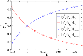
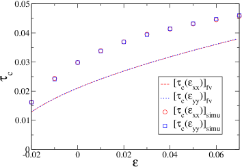
Figure 9: (Color online) Plots showing comparison of the analytically calculated values of $[y_{c}^{2}]_{fv}$ (in units of $d^{2}$) and $[\tau_{c}]_{fv}$ (in units of $\tau_{s}$) with those obtained from a free volume simulation of a single disk moving within the free volume cage. The free volume corresponds to a starting unstrained triangular lattice at $\eta=0.85$ which is then strained along $x$ or $y$ directions.

We assume that the position of the center of the moving disk $P_{0}(x,y)$, at the time of collision with any one of the six fixed disks, is uniformly distributed on the boundary $\cal{B}$ of the free-volume. Hence $[y_{c}^{2}]_{fv}$ is easily calculated using the expression:

$$[y_{c}^{2}]_{fv}=\frac{\sum_{i}\int_{{\cal{B}}_{i}}ds(y-y_{i})^{2}}{L_{\cal{B}}}~{},$$ (16)

where ${\cal{B}}_{i}$ is the part of the boundary $\cal{B}$ of the free volume when the middle disk is in contact with the $i^{\rm{th}}$ fixed disk, $ds$ is the infinitesimal length element on $\cal{B}$ while $L_{\cal{B}}$ is the total length of $\cal{B}$. Let the unstrained lattice parameters be $a_{x}^{0},~{}a_{y}^{0}=\sqrt{3}a_{x}^{0}/2$. Under strain we have $a_{x}=a_{x}^{0}(1+\epsilon_{xx})$ and $a_{y}=a_{y}^{0}(1+\epsilon_{yy})$. Using elementary geometry we can then evaluate $[y_{c}^{2}]_{fv}$ from Eq. (16) in terms of $\epsilon_{xx},~{}\epsilon_{yy}$ and the unstrained lattice parameter $a_{x}^{0}$. An exact calculation of $[\tau_{c}]_{fv}$ is nontrivial. However we expect $[\tau_{c}]_{fv}=c~{}V_{fv}^{1/2}/T^{1/2}$ where $V_{fv}$ is the “free volume” [see Fig. 8] and $c$ is a constant factor of $O(1)$ which we will use as a fitting parameter. The calculated values for $[y_{c}^{2}]_{fv}$ and $[\tau_{c}]_{fv}$ (see the appendix) are shown in Fig. 9. Also shown are their values obtained from an equilibrium simulation of a single disk moving inside the free volume cage. Thus we obtain the following estimate for the heat current:

$$[j_{y}]_{fv}=\frac{3\rho k_{B}T^{1/2}\Delta T}{L_{y}}\frac{[y_{c}^{2}]_{fv}}{c~{}V_{fv}^{1/2}}~{}.$$ (17)

We plot in Fig. (3) and Fig. (5) the above estimate of $[j_{y}]_{fv}$ along with the results from simulations. We find that the overall features of the simulation are reproduced with $c=0.42$.

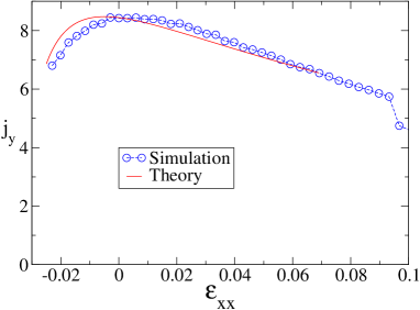
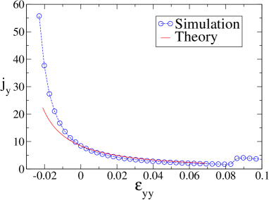
Figure 10: (Color online) Plot showing effect on $j_{y}$ of negative strains applied in the $x$ and $y$ directions. The system is prepared initially in a triangular lattice at $\eta=0.85$. Note that negative $\epsilon_{xx}$ reduces $j_{y}$ whereas negative $\epsilon_{yy}$ increases $j_{y}$.

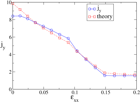
Figure 11: (Color online) Comparison of simulation results for $j_{y}$ with the approximate formula in Eq. (15) where $\tau_{c}$ and $y_{c}^{2}$ are also calculated directly from the same simulation. The results are for a $40\times 10$ system with starting value of $\eta=0.85$ and strained along $x-$direction.

For small strains we find (see the appendix) $[y_{c}^{2}(\epsilon_{xx})]_{fv}\sim 0.5+\alpha\epsilon_{xx}-\beta_{1}\epsilon_{xx}^{2}$,  $[y_{c}^{2}(\epsilon_{yy})]_{fv}\sim 0.5-\alpha\epsilon_{yy}+\beta_{2}\epsilon_{yy}^{2}$ and $[\tau_{c}]_{fv}\sim(\gamma_{1}+\gamma_{2}\epsilon-\gamma_{3}\epsilon^{2})$ where $\epsilon$ stands for either $\epsilon_{xx}$ or $\epsilon_{yy}$ and $\alpha,~{}\beta_{1},~{}\beta_{2},~{}\gamma_{1},\gamma_{2},\gamma_{3}$ are all positive constants that depend only on $a_{x}^{0}$. For $\eta=0.85$ we have $\alpha=7.62,~{}\beta_{1}=121.77,~{}\beta_{2}=124.37$ and $\gamma_{1}=0.02$, $\gamma_{2}=0.33$, $\gamma_{3}=1.125$. From these small strain scaling forms we find that $j_{y}(\epsilon_{yy})$ always decreases with positive $\epsilon_{yy}$ and increases with negative or compressive $\epsilon_{yy}$ (note that we always consider starting configurations of a triangular solid of any density). On the other hand the sign of the change in $j_{y}(\epsilon_{xx})$ will depend on the relative magnitudes of $\alpha,~{}\beta_{1}$ and $\gamma$ . For starting density $\eta=0.85$, $j_{y}(\epsilon_{xx})$ decreases both for positive and negative $\epsilon_{xx}$. In Fig. 10 we show the effect of compressive strains $\epsilon_{xx}$ and $\epsilon_{yy}$ on the heat current $j_{y}$ and compare the simulation results with the free volume theory.

It is possible to calculate $y_{c}^{2}$ and $\tau_{c}$ directly from our nonequilibrium collision time dynamics simulation. The mean collision time $\tau_{c}$ is obtained by dividing the total simulation time by the total number of collisions per colliding pair. Similarly $y_{c}^{2}$ is evaluated at every collision and we then obtain its average. Inserting these values of $\tau_{c}$ and $\langle y_{c}^{2}\rangle$ into the right hand side of Eq. (15) we get an estimate of the current as given by our theory (without making use of free-volume theory). In Fig. 11 we compare this value of the current $j_{y}$, for strain $\epsilon=\epsilon_{xx}$, and compare it with the simulation results. The excellent agreement between the two indicates that our simple theory is quite accurate.

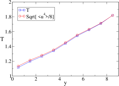
Figure 12: (Color online) Plot of temperature profile and fourth moment of velocity for a strained $40\times 10$ lattice. The unstrained packing fraction was $\eta=0.85$ and the system was strained to $\epsilon_{xx}=0.0625$.

We have also tested the assumptions of a linear temperature profile and the assumption of local thermal equilibrium (LTE) that we have used in our theory. In our simulations the local temperature is defined from the local kinetic energy density, i.e. $k_{B}T=\langle m{\bf u}^{2}/2\rangle$. Local thermal equilibrium requires a close to Gaussian distribution of the local velocity with a width given by the same temperature. The assumption of LTE can thus be tested by looking at higher moments of the velocity, evaluated locally. Thus we should have $\langle{{\bf u}}^{4}\rangle=8(k_{B}T/m)^{2}$. From our simulation we find out $\langle{{\bf u}}^{4}(y)\rangle$ and $k_{B}T(y)$ as functions of the distance $y$ from the cold to hot reservoir. The plot in Fig. 12 shows that the temperature profile is approximately linear and LTE is approximately valid. We use our theory only in the solid phase and in this case there is not much variation in the direction transverse to the direction of heat flow ($x$-direction).

Finally we have verified that heat conduction in the small confined lattice under small strains shows a linear response behaviour. This can be seen in Fig. 13 where we plot $j_{y}$ vs $\Delta T=T_{2}-T_{1}$ for a $40\times 10$ triangular lattice at $\eta=0.85$. Note that, as mentioned in the introduction, the bulk thermal conductivity of a two-dimensional system is expected to be divergent and the linear response behaviour observed here is only relevant for a finite system and in a certain regime (solid under small strain).

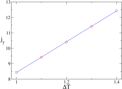
Figure 13: (Color online) Plot of $j_{y}$ vs $\Delta T=T_{2}-T_{1}$ for a $40\times 10$ triangular lattice at $\eta=0.85$. We see that the current increases linearly with the applied temperature difference.

IV Discussion

In this paper we have studied heat conduction in a two-dimensional solid formed from hard disks confined in a narrow structureless channel. The channel has a small width ($\sim 10$ particle layers) and is long ($\sim 100$ particles). Thus our system is in the nanoscale regime. We have shown that structural changes that occur when this solid is strained can lead to sudden jumps in the heat current. From the system sizes that we have studied it is not possible to conclude that these jumps will persist in the limit that the channel length becomes infinite. However the finite size results are interesting and relevant since real nano-sized solids are small. We have also proposed a free volume theory type calculation of the heat current. While being heuristic it gives correct order of magnitude estimates and also reproduces qualitative trends in the current-strain graph. This simple approach should be useful in calculating the heat conductivity of a hard sphere solid in the high density limit.

The property of large change of heat current could be utilized to make a system perform as a mechanically controlled switch of heat current. Similar results are also expected for the electrical conductance and this is shown to be true at least following one protocol of straining in Ref.my-econd . From this point of view it seems worthwhile to perform similar studies on transport in confined nano-systems in three dimensions and also with different interparticle interactions.

V acknowledgment

DC thanks S. Sengupta for useful discussions; DC also thanks RRI, Bangalore for hospitality and CSIR, India for a fellowship. Computation facility from DST grant No. SP/S2/M-20/2001 is gratefully acknowledged.

Appendix A Calculation of $[y_{c}^{2}]_{fv}$ and $V_{fv}$

Using free volume theory, as explained in the text, we get the following expressions for $[y_{c}^{2}]_{fv}$ and $V_{fv}$:

$$[y_{c}^{2}]_{fv} = \frac{1}{2}(\theta+\psi+\phi)+\frac{1}{4}\left(\sin 2\theta+\cos 2\psi-\frac{\sin 2\phi}{\theta+\psi+\phi}\right)$$

$$V_{fv} = -2(\theta+\psi+\phi)-(\sin 2\theta+\sin 2\psi-\sin 2\phi)$$ (18)

$$+ 4a_{y}\left(a_{x}-\cos\phi\right)$$

where, $\theta=\sin^{-1}(a_{x}/2)$, $\psi=\sin^{-1}(a_{x}/2-\cos\phi)$ and $\phi=\tan^{-1}(2a_{y}/a_{x})-\cos^{-1}(l/2)$ with $l=\sqrt{(a_{x}/2)^{2}+a_{y}^{2}}$ (all lengths are measured in units of $d$). For strain along $x$-direction we have $a_{x}=a_{x}^{0}(1+\epsilon_{xx})$ and $a_{y}=a_{y}^{0}~{}(=\sqrt{3}a_{x}^{0}/2)$ while for strain along $y$-direction we have $a_{y}=a_{y}^{0}~{}(1+\epsilon_{yy})$ and $a_{x}=a_{x}^{0}$. From the above expressions we can obtain Taylor expansions of $[y_{c}^{2}]_{fv}$ and $[\tau_{c}]_{fv}=cV_{fv}^{1/2}/T^{1/2}$, about the zero strain value. These give the expressions for $\alpha,~{}\beta_{1},~{}\beta_{2},~{}\gamma_{1},~{}\gamma_{2},~{}\gamma_{3}$ used in the text.

References

- (1) D. Chaudhuri and S. Sengupta, Phys. Rev. Lett. 93, 115702 (2004).
- (2) P. G. de Gennes, Langmuir 6, 1448 (1990).
- (3) J. Gao, W. D. Luedtke, and U. Landman, Phys. Rev. Lett. 79, 705 (1997).
- (4) S. Datta, Electronic transport in mesoscopic systems (Cambridge University press, Cambridge, 1997).
- (5) C. P. Poole and F. J. Owens, Introduction to nanotechnology (Wiley, New Jersey, 2003).
- (6) V. Balzani, M. Venturi, and A. Credi, Molecular devices and machines: a journey into the nano world (Wiley-VCH, Weinhem, 2003).
- (7) D. Chaudhuri and S. Sengupta, Indian Journal of Physics 79, 941 (2005).
- (8) F. Bonetto, J. Lebowitz, and L. Rey-Bellet, in Mathematical Physics 2000, edited by A. F. et al (Imperial College Pres, London, 2000), p. 128.
- (9) S. Lepri, R. Livi, and A. Polit, Phys. Rep. 377, 1 (2003).
- (10) A. Lippi and R. Livi, J. Stat Phys. 100, 1147 (2000).
- (11) P. Grassberger and L. Yang, (2002), arXiv:cond-mat/0204247.
- (12) M. P. Allen and D. J. Tildesley, Computer Simulation of Liquids (Oxford University Press, New York, 1987).
- (13) D. Chaudhuri and S. Sengupta, in preparation (unpublished).
- (14) P. Pieranski, J. Malecki, and K. Wojciechowski, Molecular Physics 40, 225 (1980).
- (15) M. Schmidt and H. Lowen, Phys. Rev. Lett. 76, 4552 (1996).
- (16) T. Chou and D. R. Nelson, Phys. Rev. E 48, 4611 (1993).
- (17) M. Schmidt and H. Lowen, Phys. Rev. E 55, 7228 (1997).
- (18) S. Datta, D. Chaudhuri, T. Saha-Dasgupta, and S. Sengupta, Europhys. Lett. 73, 765 (2006).