Also at ]L. D. Landau Institute for Theoretical Physics, Chernogolovka, Russia

Antiferromagnetism and hot spots in CeIn₃

Abstract

Enormous mass enhancement at ”hot spots” on the Fermi surface (FS) of CeIn₃ has been reported at strong magnetic field near its antiferromagnetic (AFM) quantum critical point [T. Ebihara et al., Phys. Rev. Lett. 93, 246401 (2004)] and ascribed to anomalous spin fluctuations at these spots. The ”hot spots” lie at the positions on FS where in non-magnetic LaIn₃ the narrow necks are protruded. In paramagnetic phase CeIn₃ has similar spectrum. We show that in the presence of AFM ordering its FS undergoes a topological change at the onset of AFM order that truncates the necks at the ”hot spots” for one of the branches. Applied field leads to the logarithmic divergence of the dHvA effective mass when the electron trajectory passes near or through the neck positions. This effect explains the observed dHvA mass enhancement at the ”hot spots” and leads to interesting predictions concerning the spin-dependence of the effective electron mass. The (T,B)-phase diagram of CeIn₃, constructed in terms of the Landau functional, is in agreement with experiment.

Introduction. Interest to the phenomena at quantum critical point (QCP) pervades the current literatureHertz ; Millis ; Mathur ; Paschen on intermetallic compounds. Recently the effect of magnetic fields has been studied in the antiferromagnetic (AFM) CeIn₃.HarrCeIn3 The magnetic QCP was found at $B_{c}=61T$. A strong mass enhancement observed via the de Haas - van Alphen (dHvA) effect for the electron trajectories that cross or pass close to some ”hot” spots at the Fermi surface (FS), has been reported and interpreted in terms of strong spin fluctuations at ”hot” spots implying strong many-body interactions.HarrCeIn3 It was noted that positions of these ”hot” spots coincide with the positions of the necks protruding from the similar FS for non-magnetic LaIn₃. The necks would fall close to the boundary of the AFM Brillouin Zone (BZ) for CeIn₃ and must be somehow changed or even truncated due to electron reflections at the new BZ. The AFM propagation vector $\bm{Q}=(\pi/a)(1,1,1)$ connects opposite spots on the Fermi surface.Knafo Topological changes of the FS geometry near necks, known as the Lifshitz ”2.5”-transitions, lead to weak singularities in thermodynamic and transport properties.LAK We show that at proper field directions this also affects the dHvA characteristics at ”hot” spots.

We consider dHvA effect for the three field orientations in the cubic CeIn₃ or LaIn₃. The mass enhancement was reported for two field orientations: $\bm{B}\parallel(110)$ and $\bm{B}\parallel(111)$.HarrCeIn3 In the first case the extremal electron trajectory would run across the four necks on the FS. More detailed measurements in Ref. [HarrCeIn3, ] were performed for $\bm{B}\parallel(111)$. In this case the extremal orbit does not cross ”hot” spots, but may run close if the necks‘ diameter is large enough. The dHvA measurement at $\bm{B}\parallel(100)$ when the electron trajectory passes far away from any ”hot” spot provides the non-enhanced effective mass value $m_{1}=2m_{0}$.HarrCeIn3

To start with, we explain in frameworks of a simple model, the larger masses for $\bm{B}\parallel(111)$ by the electron trajectory proximity to the saddle points, where the dHvA effective mass has a logarithmic singularity.LAK If the FS has necks, at certain orientations of the magnetic field the extremal cross-section electron trajectory passes through a saddle point (see Fig. 1).

Model calculations. We take a Fermi surface with axial symmetry along $z$-axis and narrow necks as shown in Fig. 1. For brevity we omit initially the effects of the AFM ordering and other spin effects on the ”bare” electron dispersion chosen as (we set $\hbar=1$)

$$\varepsilon({\bm{k}})=(k_{x}^{2}+k_{y}^{2})/2m_{1}+2t_{z}[1-\cos(k_{z}d)],$$ (1)

where $k_{x,y,z}$ are the momentum components along $x,y,z$ axes and $t_{z}$ is the transfer integral along $z$-direction. $k_{z}d=\pm\pi$ defines the neck positions. The Fermi surface ($\varepsilon({\bm{k}})=\varepsilon_{F}$) is given by

$$(k_{x}^{2}+k_{y}^{2})/2m_{1}-2t_{z}[1+\cos(k_{z}d)]=\Delta,$$ (2)

where $\Delta\equiv\varepsilon_{F}-4t_{z}$. The neck radius is $k_{neck}=\sqrt{2m_{1}\Delta}$. In CeIn₃ and LaIn₃ the necks are narrow, $k_{neck}d/\pi\ll 1$.

Figure 1: The Fermi surface (solid line) and the extremal electron orbit (dashed line). The saddle points due to necks are shown. The dotted lines schematically show the outer Fermi surface in CeIn₃ (see [FSCeIn3, ],[FSCeIn3N, ]).

The magnetic field ${\bm{B}}=B_{0}(sin\theta,0,\cos\theta)$ in Fig. 1 directed at angle $\theta=70.53^{\circ}$ with respect to the $z$-axis would simulate $B\parallel(111)$ in the cubic CeIn₃ where the extremal orbits, as we shall see, run rather close to the other six ”hot” spots but do not cross them.HarrCeIn3 Rotate the $x$-$z$ coordinate axes by the angle $\theta$ to make the direction of magnetic field along the $k_{z}^{\prime}$-axis:

$$\left\{\begin{array}[]{c}k_{x}=k_{x}^{\prime}\cos\theta+k_{z}^{\prime}\sin\theta\\ k_{z}=-k_{x}^{\prime}\sin\theta+k_{z}^{\prime}\cos\theta.\end{array}\right.$$ (3)

The dispersion relation (1) in the new variables is:

$$\begin{split}\varepsilon({\bm{k}}^{\prime})&=[(k_{x}^{\prime}\cos\theta+k_{z}^{\prime}\sin\theta)^{2}+k_{y}^{\prime 2}]/2m_{1}\\ &+2t_{z}\{1-\cos[d(-k_{x}^{\prime}\sin\theta+k_{z}^{\prime}\cos\theta)]\}.\end{split}$$ (4)

Electrons move along the quasi-classical trajectories of constant energy and constant $k_{z}^{\prime}$. In the dHvA effect only the electron trajectories which encircle the extremal cross-sections $S_{extr}(k_{z}^{\prime}=0)$ of the FS are important.

The effective electron mass is determined byLAK

$$2\pi m^{*}=\frac{\partial S_{extr}}{\partial\varepsilon}=\oint\frac{dk_{\perp}}{v_{\perp}}.$$ (5)

Along the trajectory of constant $\varepsilon({\bm{k}}^{\prime}),k_{z}^{\prime}$, $d\varepsilon(k_{x}^{\prime},k_{y}^{\prime})=v_{x}^{\prime}dk_{x}^{\prime}+v_{y}^{\prime}dk_{y}^{\prime}=0$, and the integral (5) rewrites as

$$2\pi m^{*}(\theta)=\oint\frac{dk_{x}^{\prime}}{v_{y}^{\prime}}=4\int_{0}^{k_{x0}}\frac{dk_{x}^{\prime}}{v^{\prime}_{y}(k_{x}^{\prime})},$$ (6)

where

$$v^{\prime}_{y}(k_{x}^{\prime})=\frac{\sqrt{2m_{1}[\Delta+2t_{z}[1+\cos(k_{x}^{\prime}d\sin\theta)]]-k_{x}^{{}^{\prime}2}\cos^{2}\theta}}{m_{1}}$$ (7)

and the integration limit $k_{x0}(\theta)$ near the necks is the solution of equation $v^{\prime}_{y}(k_{x0}^{\prime},\theta)=0$. The extremal electron trajectory passes through the saddle point if in addition to the Eqs. (7), the condition $v_{x}(\theta)|_{k^{\prime}_{y}=k^{\prime}_{z}=0,\varepsilon=\varepsilon_{F}}=0$ is satisfied. From (7) one finds the critical tilt angle $\theta_{c}$ (for narrow necks $\tan\theta_{c}\approx\pi/k_{neck}d$) corresponding to a jump of the dHvA frequency. For lower $\theta$ the electron trajectory does not pass through the saddle point. At higher tilt angles $\theta$ the electron trajectory over the necks comes to the next BZ.

Consider the case of a narrow neck. Introducing $\overline{\theta}=\pi/2-\theta$ one get for the saddle point, $\tan\overline{\theta}_{c}=k_{neck}d/2\pi\ll 1$. Taking $k^{\prime}_{z}=0$ in Eq. (3), return in (6) to the integration over $k_{z}$: $dk^{\prime}_{x}=-dk_{z}/\cos\overline{\theta}$. Expanding $v^{\prime}_{y}(k_{x}^{\prime})$ (7) near $k^{\prime}_{x0}$ at $\overline{\theta}$ close to $\overline{\theta}_{c}$, one obtains ($\delta\equiv\pi/d-k_{z}\ll 1$ and $k_{x}=-k_{z}\tan\overline{\theta}$)

$$m^{*}(\overline{\theta})=\frac{2}{\pi d}\left(\frac{m_{1}}{t_{z}}\right)^{1/2}\int_{\delta_{0}}^{\sim\frac{\pi}{d}}\frac{d\delta}{\sqrt{\delta^{2}+\left(\frac{\pi}{d}\right)^{2}\left(\frac{\overline{\theta}_{c}^{2}-\overline{\theta}^{2}}{m_{1}t_{z}d^{2}}\right)}},$$ (8)

where $\delta_{0}\equiv\left(\pi/d\right)\sqrt{(\overline{\theta}^{2}-\overline{\theta}_{c}^{2})/m_{1}t_{z}d^{2}}$, i.e. $m^{*}(\overline{\theta})$ is logarithmically divergent as

$$m^{*}(\overline{\theta})=(2/\pi)\left(m_{1}/d^{2}t_{z}\right)^{1/2}\ln\left(1/d\delta_{0}\right).$$ (9)

For $\bm{B}\parallel z$-axis in Fig.1 the dHvA oscillations in the model of Eq. (1) only measure the central (”belly”) cross section and the thickness of the ”neck”. Should we return to the cubic case and $\bm{B}\parallel(111)$, the extremal trajectories cross none of the six ”hot” spots in [[HarrCeIn3, ],Fig.3] but numerically run rather close to them (the deviation of the trajectory from the center of the ”hot spot” is given by $\overline{\theta}=19.47^{\circ}$). Thus, it becomes a question how broad are the necks to lead to a significant mass enhancement.

From the dHvA data on LaIn₃ (Fig. 4 of Ref. [LaIn3, ]) one knows the neck and ”belly” cross-section areas: $k_{neck}a=0.27$ and (for the spherical FS denoted as (d) Handbook ) $k_{F}a\approx 2.24$. Taking the value $d=2a/\sqrt{3}$ in Eq. (1), as for the cubic lattice, this gives $k_{neck}d\approx 0.32$ and $k_{F}d\approx 2.6$. The saddle points in LaIn₃ appear at the angle $\overline{\theta}_{c}\approx 5.8^{\circ}$. Hence, the necks in nonmagnetic LaIn₃ are too narrow to affect the dHvA effective mass for $\bm{B}\parallel(111)$.

In CeIn₃ the ”belly” radius $k_{F}$ is very close to the one in LaIn₃, while the neck cross-section area depends on the AFM order parameter and the value of magnetic field (in addition, the bands become spin split, see below). At field $B=15T$, the dHvA frequency from the neck (the (j)-orbit) is about $3$ times larger than in LaIn₃,FSCeIn3 which would give $k_{neck}d\approx 0.55$ and $\overline{\theta}_{c}\approx 10^{\circ}$. It is still rather far from the tilt angle $\overline{\theta}_{0}=19.47^{\circ}$. However, according to Refs. [HarrCeIn3, ; FSCeIn3N, ] the neck radius is considerably higher. Then the neck radius may reach and overpass the critical value $k_{neck}^{crit}d\approx 1.1$ when $\overline{\theta}_{c}=\overline{\theta}_{0}$ for the extremal orbit to pass through the saddle point at the field $\bm{B}\parallel(111)$. There are no data on the field dependence of the neck radius in CeIn₃ so far.

If $\bm{B}$ is perpendicular to the plane in Fig.1 for our model (1), the extremal trajectory would run along the FS shown in Fig.1. The mass enhancement would be determined by the neck‘s width $m^{*}\approx 2m_{1}\sqrt{2\hbar^{2}/t_{z}m_{1}d^{2}}\ln(2\pi\sqrt{t_{z}/\Delta})$. In the cubic CeIn₃ this would correspond to $\bm{B}\parallel(110)$: four necks‘ singularities would provide strong mass enhancement, as stated in Ref. [HarrCeIn3, ]. Strictly speaking, the dHvA frequency for the (d)-FS should be observable only at strong band splitting, as we discuss below.

CeIn₃ and other REIn₃. The FS‘es in CeIn₃ are now known in some main details.HarrCeIn3 ; FSCeIn3 ; FSCeIn3N The two most remarkable features are common with nonmagnetic LaIn₃LaIn3 : 1)a practically spherical FS sheet (denoted as (d)Handbook ; FSCeIn3 ; FSCeIn3N ; Umehara ) with the diameter in the k-space close to the AFM vector $\bm{Q}=(\pi/a)(1,1,1)$; 2) ”necks” protruding from FS sheet (d) towards an outer FS.FSCeIn3 ; FSCeIn3N The dHvA orbits and FS‘s for necks were labeled as (j); their sizes vary among the REIn₃ group.Handbook ; Umehara Analysis of the dHvA oscillations, as well as the electron-positron annihilation experiments in the paramagnetic phaseFSCeIn3 ; FSCeIn3N confirm the localized character of the Ce f-electrons.Knafo ; Walker ; CePd2Si2 The moment J=5/2 in the cubic environment is split into the quartet, $\Gamma_{8}$ and the Kramers‘ doublet $\Gamma_{7}$; the latter is responsible for the AFM ordering in CeIn₃ Knafo . The propagating vector $\bm{Q}$ corresponds to the staggered magnetization, $\bm{S}_{\perp}(\bm{Q})$, aligned antiferromagnetically perpendicular to the adjacent $(111)$ ferromagnetic planes.Walker Magnetic anisotropy seems to be weakCePd2Si2 and is neglected below.

CeIn₃ is a moderate HF material with the Sommerfeld‘s $\gamma=130mJ/K^{2}$mole. At the ambient pressure the Neel temperature is $T_{N}=10K$. The staggered magnetization is close to the value 0.71$\mu_{B}$ expected for localized $\Gamma_{7}$ doublet (see in Ref. [HarrCeIn3, ]). The AFM state can be suppressed by applied pressure $P_{c}\approx 26$ kbar.Endo In the vicinity of this pressure the coexistence of AFM order and superconductivity has been reported.Mathur The magnetic QCP in CeIn₃ was found at the field $B\approx 61T$.HarrCeIn3 As it was said above, the authors claimed strong many-body effects at ”hot” spots on the FS sheet (d).HarrCeIn3

AFM order in CeIn₃. For common antiferromagnets strong enough applied field destroys the Neel state by aligning staggered moments parallel to the field, $\bm{B}$. For CeIn₃ $T_{N}=10K$ looks already rather low, so that one may attempt apply the Landau mean-field approach:LL1

$$F(T,B)=a(T-T_{N})\bm{S}_{\perp}^{2}+b\bm{S}_{\perp}^{4}-\frac{\chi\bm{B}^{2}}{2}+\eta(\bm{B}\bm{S}_{\perp})^{2}+\eta^{\prime}\bm{B}^{2}\bm{S}_{\perp}^{2}$$ (10)

where $\bm{S}_{\perp}$ is the local spin component along the staggered magnetization vector (only terms independent on the crystal anisotropy left in Eq. (10)). From Eq. (10) the quadratic dependence $T_{N}(B)=T_{N}[1-(B/B_{c})^{2}]$ immediately follows, reproducing the results on Fig.1a of Ref. [HarrCeIn3, ] with high accuracy. This agrees with the assumption that magnetic anisotropy is indeed low. The dHvA mass for the (d) sheet away from the singular field orientations is also rather low: $m^{*}\approx 2m_{e}$.HarrCeIn3 Therefore, we assume that AFM order and the phenomena studied in Ref. [HarrCeIn3, ] are only weakly linked to other Kondo-like features of CeIn₃: i.e., the (d) and (j) FS pieces are weakly coupled to the f-electrons. Next question is whether one can explain low $T_{N}=10K$ for CeIn₃ via the RKKY mechanism with the help of (d)-sheet only. The diameter of the (d)-sheet equals to the $\bm{Q}$ vector value and, hence, is capable to provide the commensurate RKKY interaction. It is also known that parameters for these FS‘es are not dramatically different for the rest of REIn₃ family.Handbook From Eq. (10) it follows that $|\bm{S}_{\perp}|(\bm{Q})\approx(1-T/T_{N})^{1/2}$ ,(at $B=0$), and $|\bm{S}_{\perp}|=(1-(B/B_{c})^{2})^{1/2}$ at $T=0$.

Energy spectrum near hot spots at non-zero $B$ and $|\bm{S}_{\perp}|$. Introduce the exchange term $J\hat{\bm{\sigma}}\bm{S}_{i}$ between itinerant and localized spins. This exchange leads to the RKKY interaction between localized spins. It can be estimated as $J\sim\sqrt{T_{N}/\nu_{F}}$, where $\nu_{F}$ is the density of states at the Fermi level. Assuming that only the (d)-parts of electron spectrum contribute to the RKKY interaction we obtain $\nu_{F}\approx 3/2\varepsilon_{F}\approx 3m_{1}/k_{belly}^{2}=1/3000K$. This gives $J\approx 170K$. Therefore, at all $\bm{B}$, $\mu_{B}B\ll J$.

The effective magnetic field acting on electrons is

$$\mu_{B}\bm{B}_{eff}=\mu_{B}\bm{B}+J\bm{S}_{\parallel},$$ (11)

where $\bm{S}_{\parallel}$ is the local spins’ component parallel to $\bm{B}$. Let $\hat{\bm{n}}_{S}$ and $\hat{\bm{n}}_{B}$ be the two perpendicular (in absence of anisotropy) unit vectors of Pauli matrices for the directions of $\bm{S}_{\perp}$ and $\bm{B}$ correspondingly. Then with $\bm{Q}$ being the AFM propagation vector, the new energy spectrum in AFM phase is determined from two equations for the electronic states $(\bm{k},\bm{k+Q})$:

$$\left\{\begin{array}[]{c}(\hat{E}-\hat{\varepsilon}_{\bm{k}}+\hat{\bm{n}}_{B}\mu_{B}\bm{B}_{eff})\Psi_{\bm{k}}=-J\hat{\bm{n}}_{S}\bm{S}_{\perp}\Psi_{\bm{k}+\bm{Q}}\\ (\hat{E}-\hat{\varepsilon}_{\bm{k}+\bm{Q}}+\hat{\bm{n}}_{B}\mu_{B}\bm{B}_{eff})\Psi_{\bm{k}+\bm{Q}}=-J\hat{\bm{n}}_{S}\bm{S}_{\perp}\Psi_{\bm{k}}.\end{array}\right.$$ (12)

Multiplying both equations by $\hat{\bm{n}}_{S}$ and excluding $\Psi_{\bm{k}+\bm{Q}}$ one obtains the equation in the spin space:

$$\begin{array}[]{c}(\hat{E}-\hat{\varepsilon}_{\bm{k}+\bm{Q}}-\hat{\bm{n}}_{B}\mu_{B}\bm{B}_{eff})\\ \times(\hat{E}-\hat{\varepsilon}_{\bm{k}}+\hat{\bm{n}}_{B}\mu_{B}\bm{B}_{eff})\Psi_{\bm{k}}=J^{2}|\bm{S}_{\perp}|^{2}\Psi_{\bm{k}}\end{array}$$ (13)

The four energy branches from (13) are

$$E_{k,\sigma}^{\pm}=\frac{\varepsilon_{k}+\varepsilon_{k+Q}}{2}\pm\sqrt{\left(\frac{\varepsilon_{k}-\varepsilon_{k+Q}}{2}-\mu_{B}B_{eff}\sigma\right)^{2}+J^{2}S_{\perp}^{2}}.$$ (14)

If the vector $\bm{Q}$ exactly connects two opposite necks in Fig. 1, one obtains near the necks

$$E_{k,\sigma}^{\pm}=\varepsilon_{k}\pm\sqrt{\left(\mu_{B}B_{eff}\right)^{2}+J^{2}|S_{\perp}|^{2}}.$$ (15)

Above $B_{c}$ the two branches go over into the Zeeman splitting with the effective field from Eq. (11) and $S_{\parallel}=1$. For convenience, we normalize $|\bm{S}_{\parallel}|^{2}+|\bm{S}_{\perp}|^{2}=1$. Then substituting Eq. (11) to (15) we obtain at $\mu_{B}B\ll J$

$$E_{k,\sigma}^{\pm}\approx\varepsilon_{k}\pm(J+\mu_{B}\bm{B}\,\bm{S}_{\parallel}).$$ (16)

The AFM order adds new features to the electron dispersion and the Fermi surface of the model (1). With signs ($\pm$) there are now two branches shown in Fig. 2. For the sign (+) the dHvA experiment at $B\ll B_{c}$ would see the decrease of the necks’ width as compared to the bare spectrum (i.e., without AFM order). If $\Delta=k_{neck}^{2}/2m_{1}<J$, these necks in the (d)-part of the FS are completely destroyed, as shown in Fig. 2. Otherwise, these necks would only be narrowed. For the sign (-) the necks’ width increases due to AFM ordering.

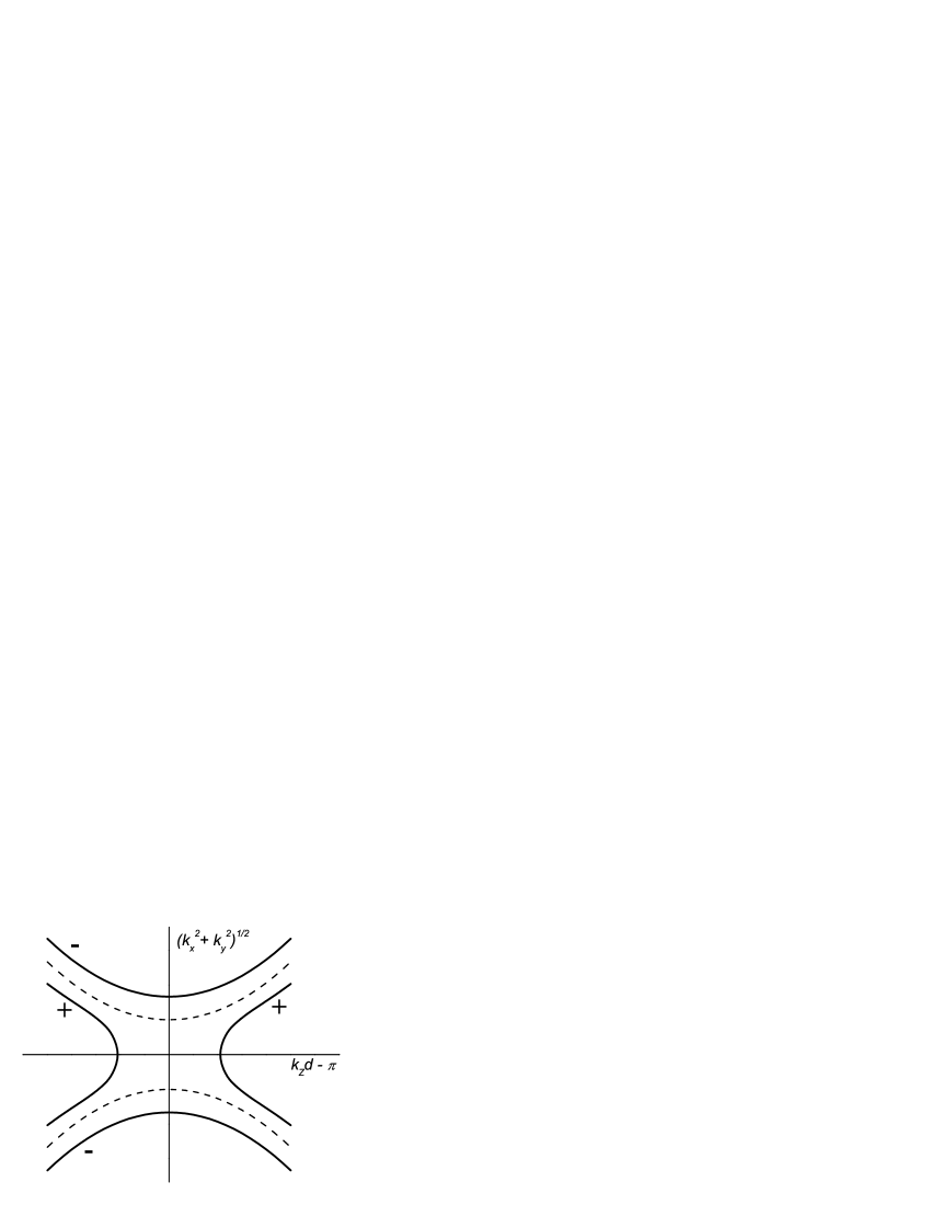
Figure 2: Schematic view of the Fermi surface at the neck with (solid line) and without (dashed line) AFM order. The ($\pm$) signs on the figure correspond to the ($\pm$) signs in Eq. (14)

The authors of Ref. [HarrCeIn3, ] have used the width of the necks $\approx 1/12$ of the orbit circumference. This is close to the data of Ref. [FSCeIn3N, ] but disagree with the estimations of Ref. [FSCeIn3, ]. Using data of Ref. [FSCeIn3N, ] we would get $\Delta$ comparable to $J$. If so, one may indeed relate the mass enhancement mechanism for $\bm{B}\parallel(111)$ described above to the broadening of the gap between two outer (-) trajectories in Fig. 2. This broadening depends on the magnetic field as described by Eq. (16). At $J=170K$ and $B=60T$ this term is $\approx 0.4J$. The estimates we have done for $\Delta$,$J$ show that it is realistic to account for the observed mass enhancement at $\bm{B}\parallel(111)$. On the other hand, we must repeat that there are no experimental data for a quantitative fit because so far no attempt have been made to account for the band splitting and the field dependence of the dHvA frequencies corresponding to the j-orbits on the Fermi surface (the necks).

Band splitting and the dHvA experiments. At high magnetic field (above $B_{c}$) the effective Zeeman splitting (11) (with $|\bm{S}_{\parallel}|=1$) results in the spin dependence of the energy spectrum and of the neck width. The Zeeman splitting makes the necks thicker for one spin component and thinner for the other, which leads to the spin-dependence of the effective mass, as mentioned above. This spin dependence can be observed for both (110) and (111) magnetic field directions. In particular, for the direction $\bm{B}\parallel(111)$ the saddle point logarithmic divergence of the effective mass is possible for only one spin component (sign (-) in Fig. 2). With farther increase of magnetic field (assuming $J>0$), this spin component ceases to contribute to the dHvA signal with this frequency at all since the electron trajectories start to leave the (d)-sheet of the FS. This can be experimentally verified.Endo At $\bm{B}\parallel(110)$ one expects similar behavior, except the (-) spin component at this field direction, ceases to contribute to old dHvA frequency at lower field than at $\bm{B}\parallel(111)$. At $B<B_{c}$ the splitting of the energy spectrum remains, but now $|\bm{S}_{\parallel}|=\sqrt{1-|\bm{S}_{\perp}|^{2}}=B/B_{c}$. Although, in Ref. [HarrCeIn3, ] the spin dependence (or the band splitting) of the effective mass was not studied, it has been observed rather definitely in CeIn₃ under pressure.Endo

More remarkable effect for $\bm{B}\parallel(110)$ is that the two signs in Eq. (15) would correspond to two different dHvA frequencies. If one of the necks is broken (sign (+) in Fig. 2), one of the dHvA frequencies corresponds to the trajectory encircling the (d)-sheet of FS. Of the utmost importance are the dHvA experiments measuring explicitly the frequency(ies) from the j-trajectories on the FS as a function of the field (for $\bm{B}\parallel(111)$, i.e. along the direction of the neck), that would confirm the band structure of the AFM CeIn₃, constructed in this paper.

To summarize, by making use of the peculiar shape of the energy spectrum of CeIn₃ in terms of spherical (d) and neck-like (j) Fermi surfaces, we have constructed the full (T-B) phase diagram for antiferromagnetism in this compound in agreement with the experiments.HarrCeIn3 We have analyzed the interplay between antiferromagnetism and external magnetic field at the neck positions and semi-quantitatively explained the observed enhancement of the electron effective mass at the so-called ”hot spots”.HarrCeIn3 We emphasize the importance of the ”2.5” Lifshitz phase transition between magnetic CeIn₃ and nonmagnetic LaIn₃. It was our intention to show that the details of the Fermi surface topology are important for CeIn₃, although the magnetic quantum criticality in other heavy fermion materials may bear the universal character. A few straightforward experiments are suggested to verify the above ideas.

Acknowledgements. One of the authors (LPG) thanks T.Ebihara and N.Harrison for explanations regarding the electron spectrum in CeIn₃. He benefited from the fruitful discussions with Z.Fisk about antiferromagnetism and Kondo effect in Ce-compounds. The work was supported by NHMFL through the NSF Cooperative agreement No. DMR-0084173 and the State of Florida, and (PG) by DOE Grant DE-FG03-03NA00066.

References

- (1) J.A.Hertz, Phys. Rev. B 14, 1165 (1976).
- (2) A.J. Millis, Phys. Rev. B 48, 7183 (1993).
- (3) N.D. Mathur, F. M. Grosche, S. R. Julian et al., Nature 394, 39 (1998).
- (4) S. Paschen et al., Nature 432, 881 (2004).
- (5) Takao Ebihara, N. Harrison, M. Jaime, Shinya Uji, and J. C. Lashley, Phys. Rev. Lett. 93, 246401 (2004).
- (6) W. Knafo et al., J. Phys. Cond. Mat. 15, 3741 (2005).
- (7) I.M. Lifshitz, M.Ya. Azbel, M.I. Kaganov, Electron theory of metals, New York - London, 1973.
- (8) M. Biasini, G. Ferro, and A. Czopnik, Phys. Rev. B 68, 094513 (2003).
- (9) J. Rusz and M. Biasini, Phys. Rev. B 71, 233103 (2005).
- (10) Isuru Umehara, Nobuyuki Nagai and Yoshichika Onuki, J. Phys. Soc. Jpn. 60, 591 (1991).
- (11) L. D. Landau and E. M. Lifshitz, Course of Theoretical Physics, Vol. 8: Electrodynamics of Continuous Media, (Nauka, Moscow, 2001; Pergamon Press, Oxford, 1984).
- (12) Y. Onuki and A. Hasegawa, Handbook on Phys. and Chem. of Rare Earth (1995), Vol. 20, Chap. 135.
- (13) I. Umehara, T. Ebihara, N. Nagai et al., J. Phys. Soc. Jpn. 61, 19 (1992); T. Ebihara, I. Umehara, A.K. Albessard et al.,ibid, 61, 1473 (1992).
- (14) I.R. Walker et al., Physica C 282-287, 303 (1997).
- (15) I. Sheikin et al., Phys. Rev. B 67, 094420 (2003).
- (16) M. Endo, N. Kimura, H. Aoki et al., Phys. Rev. Lett. 93, 247003 (2004).