Columnar and lamellar phases in attractive colloidal systems

Abstract

In colloidal suspensions, at low volume fraction and temperature, dynamical arrest occurs via the growth of elongated structures, that aggregate to form a connected network at gelation. Here we show that, in the region of parameter space where gelation occurs, the stable thermodynamical phase is a crystalline columnar one. Near and above the gelation threshold, the disordered spanning network slowly evolves and finally orders to form the crystalline structure. At higher volume fractions the stable phase is a lamellar one, that seems to have a still longer ordering time.

In colloidal suspensions solid (or liquid) mesoscopic particles are dispersed in another substance. These systems, like blood, proteins in water, milk, black ink or paints, are important in our everyday lives, in biology and industry russel ; morrison . It is crucial, for example, to control the process of aggregation in paint and paper industries lu , or to favour the protein crystallization in the production of pharmaceuticals and photonic crystals muschol ; mcpherson .

A practical and exciting feature of colloidal suspensions is that the interaction energy between particles can be well controlled pusey ; stradner ; anderson . In fact particles can be coated and stabilized leading to a hard sphere behaviour, and an attractive depletion interaction can be brought out by adding some non-adsorbing polymers. The range and strength of the potential are controlled respectively by the size and concentration of the polymer anderson ; edinburgh . Recent experimental works highlighted the presence of a net charge on colloidal particles stradner ; bartlett giving rise to a long range electrostatic repulsion in addition to the depletion attraction.

The competition between attractive and repulsive interactions produces a rich phenomenology and a complex behavior as far as structural and dynamical properties are concerned. For particular choices of the interaction parameters, the aggregation of particles is favoured but the liquid-gas phase transition can be avoided and the cluster size can be stabilized at an optimum valuegron . Experimentally, such a cluster phase made of small equilibrium monodisperse clusters is observed using confocal microscopy at low volume fraction and low temperature (or high attraction strength) weitzclu ; bartlett ; stradner . Increasing the volume fraction, the system is transformed from an ergodic cluster liquid into a nonergodic gel weitzclu ; bartlett , where structural arrest occurs. Using molecular dynamic simulations, we showed that such structural arrest is crucially related to the formation of a long living spanning cluster, providing evidence for the percolation nature of the colloidal gel transition at low volume fraction and low temperature noi_me ; noi . This scenario was confirmed by recent experiments bartlett and molecular dynamics simulationssciort , where it was shown that increasing the volume fraction clusters coalesce into elongated structures eventually forming a disordered spanning network. A realistic framework for the modelization of these systems is represented by DLVO interaction potentials israel , which combine short-range attractions and long-range repulsions. A suited choice of DLVO models has in fact allowed to reproduce, by means of molecular dynamics calculations, many experimental observations, like the cluster phase and the gel-like slow dynamics noi_me ; noi ; sciort .

On the other hand, competing interactions have been studied in many other systems, ranging from spin systems to aqueous surfactants or mixtures of block copolymers, and often lead to pattern formation or to the creation of periodic phases lamellar ; cao ; sear ; muratov ; reatto ; marco ; surf .

In this paper, we simulate by molecular dynamics a system composed of monodisperse particles, interacting with a short range attraction and a long range repulsion in analogy with DLVO models, for a large range of temperatures and volume fractions. At low temperature, increasing the volume fraction in the region of phase space where the system forms a percolating network and waiting long enough, we observe that the system spontaneously orders, to form a periodic structure composed by parallel columns of particles. This finding strongly suggests that the transition to the gel phase, observed in experiments and in numerical simulations, happens in a “supercooled” region, namely in a disordered phase which is metastable with respect to crystallization. This is supported also by the results on a mean field model marco . We then study the phase diagram of the system, by evaluating the free energy of the disordered and ordered phases, and find the region where the columnar phase is stable. We also locate the region of phase space where the stable phase is the lamellar one. Such phase does not form spontaneously within the observation times, therefore indicating a much longer nucleation time.

We have considered a system made of $1300\leq N\leq 2300$ particles. The particles interact through the effective interaction potential noi :

$$V(r)=\epsilon\left[a_{1}\left(\frac{\sigma}{r}\right)^{36}-a_{2}\left(\frac{\sigma}{r}\right)^{6}+a_{3}e^{-\lambda(\frac{r}{\sigma}-1)}\right],$$ (1)

where $a_{1}=2.3$, $a_{2}=6$, $a_{3}=3.5$, and $\lambda=2.5$. The potential is truncated and shifted to zero at a distance of 3.5$\sigma$. The temperature $T$ is in units of $\epsilon/k_{B}$, where $k_{B}$ is the Boltzmann constant. The number of particles varies as we consider different volume fractions, defined using the equivalent system of spheres of diameter $\sigma$ as $\phi=4/3\pi\sigma^{3}N/L^{3}$ in a simulation box of size $L$. We have performed Newtonian molecular dynamics at constant NVT using the velocity Verlet algorithm and the Nosé-Hoover thermostat hoover with time step $\Delta t=0.01t_{0}$ (where $t_{0}=\sqrt{m\sigma^{2}/\epsilon}$ and $m$ is the mass of the particles). For a given volume fraction $\phi$, the system is first thermalized at very high temperature and then quenched to the desired temperature. We let it evolve for times ranging between $10^{5}\,t_{0}$ and $10^{6}\,t_{0}$ ($10^{7}$–$10^{8}$ MD steps).

At low volume fraction ($\phi<0.2$) and high temperature ($T>0.25$), the system remains in a disordered configuration during the simulation time window. Decreasing the temperature, we observe the formation of long living clusters with a typical size of about ten particles. At temperature $T=0.25$ and for volume fractions $\phi$ between $0.15$ and $0.23$, we find that, shortly after the quench, these clusters aggregate into locally rod-like structures with a length from a few to about ten molecular diameters which finally coalesce into a disordered network. At longer times, between $5\times 10^{4}\,t_{0}$ and $10^{6}\,t_{0}$, these elongated rod-like structures start to spontaneously order in a two-dimensional hexagonal packing of parallel columnar structures, with a fast drop in the energy, as illustrated in Fig. 1(a). We also observe that locally particles rearrange in a spiral structure which optimizes the competing interactions, very similar to the Bernal spiral bernal , where each particle has six neighbors. Such a local structure is also indicated by experimental observations bartlett and found in numerical simulations with similar interactions sciort .

Figure 1: a) Snapshot of one of the systems after the ordering (simulation time $t=10^{5}t_{0}$), taken from a direction parallel to the columns, showing the two-dimensional arrangement of the axes. Since columns are not perfectly straight, their diameters appear to be larger than in reality; b) Lamellar phase at $\phi=0.26$ and $T=0.2$.

In order to infer the phase diagram of the system at low volume fraction, we first studied the state of the system at very low temperature. In that limit, entropy can be neglected and the equilibrium state of the system should be the crystalline structure with the lowest potential energy. Of course, an exact determination of such a structure, that may depend on the volume fraction, is far from trivial. We have instead selected a few possible structures and made a comparative analysis by calculating numerically their potential energy as a function of the volume fraction. The structures considered are the following (in each case, the lattice spacing between elements is chosen to provide the desired volume fraction):

1) Cluster crystal: Three-dimensional hexagonal close packing of nearly spherical clusters, each cluster being composed of thirteen particles (a central one in contact with twelve external ones). In this case particles have 5.54 neighbors on the average. These clusters were chosen because of their similarity to the long-living clusters observed at low temperature and volume fraction, composed generally by one particle surrounded by eight to eleven neighbors.

2) Columnar phase: Two-dimensional hexagonal packing of parallel Bernal spirals. In this case, each particle has six neighbors.

3) Lamellar phase: Parallel planes, each plane being formed by one or more layers of hexagonally packed particles (Fig. 1(b)). In this case, the average number of neighbors per particle is between six (one layer) and twelve (when the number of layers increases the structure becomes an hexagonal close-packed lattice of particles).

After having placed the particles to form these structures with the distance between nearest neighbors corresponding to the minimum of the pair-potential, we have calculated the nearest minimum of the potential energy landscape, by minimizing the total potential energy $U({\bm{r}}_{1},\ldots,{\bm{r}}_{N})$ as a function of the particle positions, using a conjugate-gradient algorithm nrc . The potential energy per particle $U_{0}/N$ of the minimum is shown in Fig.2.

The cluster crystal never provides the lowest energy because of the limited number of neighbors per particle. For volume fractions $\phi<0.235$, the columnar phase of Bernal spirals is energetically preferred. Indeed, in this case the combination of a relatively high number of first neighbors and a low number of second and third neighbors minimizes the repulsive part of the interaction potential. Increasing the volume fraction, the columns get closer and the repulsion between them becomes relevant. At $\phi>0.235$, the potential energy of the columnar phase becomes higher than that of the two-layer lamellae. In fact, since lamellae are more distant than columns for a given volume fraction, the repulsion between lamellae is weaker. It is interesting to note that one-layer lamellae are never energetically preferred and that their minimum potential energy becomes close to the one of the columns at high volume fraction. At $\phi>0.42$, the three-layer lamellae exhibit the lowest potential energy, and so on. Similar results were recently found in a $2d$ DLVO system reatto .

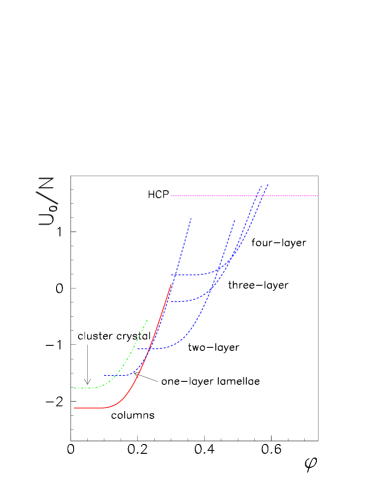
Figure 2: Minimum of the total potential energy per particle, $U_{0}/N$, for several structures as a function of the volume fraction.

In order to test the stability of these structures as the temperature increases, we performe the following experiment. Given a volume fraction and a temperature, we let evolve a crystalline configuration of columns or two-layer lamellae by means of molecular dynamics at constant temperature for $10^{6}t_{0}$. The obtained phase diagram is shown in Fig. 3. Circles represent state points where both columns and lamellae break down before the end of the simulation (disordered phase). Triangles are the points where lamellae break down, but columns are stable (columnar phase). Squares are the points where lamellae are stable and columns break down (lamellar phase). Finally, the points where triangles and squares overlap correspond to the states where both columns and lamellae remain stable until $t=10^{6}t_{0}$. We note that near the boundaries with the disordered phase, columns or lamellae become fuzzy, but the modulation of the density is still clearly visible.

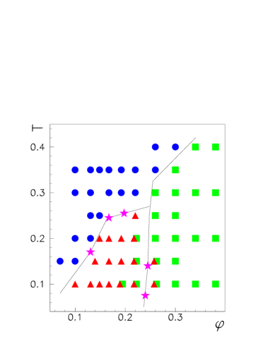
Figure 3: $T$-$\phi$ phase diagram of the system. Circles represent the disordered phase, triangles the columnar phase and squares the lamellar phase. Stars represent points where the calculated free energy of the two phases crosses. Solid lines are a guide for the eyes.

To check the results found by molecular dynamics simulations and to better estimate the phase boundaries, we have computed the free energy of the three phases that seem to be relevant for $\phi<0.4$: disordered phase, columnar phase, and two-layer lamellar phase. The free energy of the disordered phase is computed by thermodynamic integration thermo along the following path: from the perfect gas limit ($V\to\infty$) down to the desired volume $V$ along the isotherm $T_{0}=1$. The free energy at $(V,T_{0})$ is therefore given by

$$\frac{F_{0}}{NT_{0}}=\ln\left(\frac{N}{V}\right)+\frac{3}{2}\ln\left(\frac{2\pi\hbar^{2}}{mT_{0}}\right)-1+\int\limits_{V}^{\infty}\frac{\Delta P(V^{\prime})}{NT_{0}}\,dV^{\prime}$$ (2)

where $\Delta P(V)=P(V)-\frac{NT_{0}}{V}$ is the excess pressure with respect to the perfect gas. Since values of $\hbar$ and the mass $m$ merely shift the free energy by a constant, we set $\hbar=1$ and $m=1$. We have then integrated along the isochore $V$, from $T_{0}$ to the desired temperature, and obtained

$$\frac{F}{NT}=\frac{F_{0}}{NT_{0}}+\frac{3}{2}\ln\left(\frac{T_{0}}{T}\right)+\int\limits_{T}^{T_{0}}\frac{U(T^{\prime})}{N{T^{\prime}}^{2}}\,dT^{\prime}.$$ (3)

Starting from $T=0$, we have calculated the free energy of the two crystalline phases by integrating along an isochore. At very low temperatures the potential energy landscape can be approximated by a parabolic function

$$U=U_{0}+\frac{1}{2}\sum_{i=1}^{3N}\lambda_{i}x_{i}^{2},$$ (4)

where $\lambda_{i}$ are the eigenvalues of the Hessian matrix at the minimum of the potential. The free energy is then calculated as

$$\frac{F}{NT}=\frac{U_{0}}{NT}+\frac{1}{2}\sum_{i=1}^{3N}\ln\lambda_{i}+\frac{3}{2}\ln\left(\frac{\hbar^{2}}{mT^{2}}\right)-\int\limits_{0}^{T}\frac{\Delta U(T^{\prime})}{N{T^{\prime}}^{2}}\,dT^{\prime},$$ (5)

where $\Delta U(T)=U(T)-U_{0}-\frac{3NT}{2}$.

In Fig. 4 the free energy of the disordered phase and of the columnar phase at $\phi=0.1308$ are shown as a function of the temperature. The curves cross at the temperature ($T_{c}=0.17$) corresponding to the first order transition from the columnar phase to the disordered phase. This, together with the other transition points, are marked in Fig. 3 by a star nota2 .

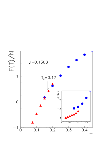
Figure 4: Free energy per particle $F(T)/N$ of the disordered phase (circles) and of the columnar phase (triangles) as a function of temperature at $\phi=0.1308$. Inset: potential energy per particle $U(T)/N$.

These results suggest the following scenario for colloidal gelation at low volume fraction and low temperature. Just remind that in real colloidal systems the control parameter corresponding to low temperature is a high effective attraction strength. The competition between attractive and repulsive interaction induces a typical modulation length clearly detected at very low volume fraction in the cluster phase. As the volume fraction is increased, clusters are prone to aggregate in spite of the long-range repulsion. This results in the growing of elongated structures which keep track of the modulation length. Eventually, a modulated phase forms, with a columnar geometry or a lamellar one at higher volume fraction. Of course the precursors of the modulated structures will have defects such as local inhomogeneities and branching points. Furthermore, the slow dynamics due to the viscosity of the solvent and to the imperfect shape of the particles may also hinder the ordered phase, producing long-living metastable disordered states. Hence, when the volume fraction is high enough, an interconnected spanning structure is formed and a gel-like behavior is observed as it is frequently the case in the experiments.

The authors thank Gilles Tarjus for interesting discussions and for pointing out the existence of lamellar phases in systems with competing interactions. The research is supported by MIUR-PRIN 2004, MIUR-FIRB 2001, CRdC-AMRA, the Marie Curie Reintegration Grant MERG-CT-2004-012867 and EU Network Number MRTN-CT-2003-504712.

References

- (1) W. B. Russel, D. A. Saville, and W. R. Schowalter, “Colloidal Dispersions”, Cambridge University Press, Cambridge (1989).
- (2) “Colloidal dispersions : suspensions, emulsions, and foams”, Ian D. Morrison, Sydney Ross (New York , Wiley-Interscience, 2002).
- (3) C. Lu and R. Pelton, J. Colloid Interface Sci, 254, 101 (2002).
- (4) M. Muschol and F. Rosenberger, J. Chem. Phys. 107, 1953 (1997).
- (5) A. McPherson, Preparation and analysis of protein crystals (Kieger Publishing, Malabar 1982).
- (6) P. N. Pusey, Proceedings of Les Houches (1986) pp. 765-937.
- (7) A. Stradner et al. Nature 432, 492 (2004).
- (8) V.J. Anderson and H.N.W. Lekkerkerker, Nature 416, 811 (2002).
- (9) W. C. Poon et al., Physica A 235, 110 (1997).
- (10) A.I.Campbell et al, Phys. Rev. Lett. 94, 208301 (2005); R. Sanchez and P. Bartlett, cond-mat/0506566 (2005).
- (11) J. Groenewold and W. K. Kegel, J. Phys. Chem. B 105, 11702 (2001).
- (12) P. N. Segré, V. Prasad, A. B. Schofield, and D. A. Weitz, Phys. Rev. Lett. 86, 6042 (2001); A. D. Dinsmore and D. A. Weitz, J. Phys. : Condens. Matter 14, 7581 (2002).
- (13) A. Coniglio et al., J. Phys. C: Condens. Matter 16,S4831 (2004).
- (14) A. de Candia et al, Physica A 358, 239 (2005).
- (15) F. Sciortino, P. Tartaglia and E. Zaccarelli, J. Phys. Chem. B 109, 21942 (2005); S. Mossa et al Langmuir 20, 10756 (2004).
- (16) J.N. Israelachvili, “Intermolecular and surface forces”, Academic press (London) 1985; J. C. Crocker and D. G. Grier, Phys. Rev. Lett. 73, 352 (1994).
- (17) M. Seul and D. Andelman, Science 267, 476 (1995); C.M. Knobler and R.C. Desai, Annu. Rev. Phys. Chem. 43, 207 (1992); L. Leibler, Macromolecules 13, 1602 (1980); V. J. Emery and S. A. Kivelson, Physica C 209, 597 (1993); D. Kivelson et al., Physica A 219, 27 (1995); J. Schmalian and P. G. Wolynes, Phys. Rev. Lett. 85, 836 (2000). M. Grousson, V. Krakoviack, G. Tarjus and P. Viot, Phys. Rev. E 66, 026126 (2002).
- (18) J. Wu and J. Cao, J. Phys. Chem. B 109, 21342 (2005); cond-mat/0602428.
- (19) R. P. Sear et al, Phys. Rev. E 59, R6255 (1999).
- (20) C. B. Muratov, Phys. Rev. E 66, 066108 (2002).
- (21) M. Tarzia and A. Coniglio, cond-mat/0506485 (2005).
- (22) S-H. Chen et al, Phys. Rev. E 54, 6526 (1996); S-H. Chen et al, Phys. Rev. Lett. 86, 740 (2001).
- (23) A. Imperio and L. Reatto, J. Phys.: Condensed Matter 16, S3769 (2004).
- (24) M.P. Allen and D.J. Tildesley, “Computer Simulation of Liquids”, Oxford University Press, (1987).
- (25) J.D. Bernal, Proc. Royal Soc. (London) A 299, 280 (1964).
- (26) D. Frenkel and B. Smit, “Understanding molecular simulation”, Academic Press, 2001.
- (27) W.H. Press, B.P. Flannery, S.A. Teukolsky, W.T. Vetterling, “Numerical Recipes in C”, Cambridge University Press, 2nd ed. (1992).
- (28) In principle, the first order transition line can be calculated also with the Clausius-Clapeyron equation , where and are the pression and energy differences between the two phases. However, in this way the result depends entirely on quantities evaluated at the transition, where the fluctuations and hence the errors are large.