Spin tunneling through an indirect barrier

Abstract

Spin-dependent tunneling through an indirect bandgap barrier like the GaAs/AlAs/GaAs heterostructure along [001] direction is studied by the tight-binding method. The tunneling is characterized by the proportionality of the Dresselhaus Hamiltonians at $\Gamma$ and $X$ points in the barrier and by Fano resonances (i.e. pairs of resonances and anti-resonances or zeroes in transmission). The present results suggest that large spin polarization can be obtained for energy windows that exceed significantly the spin splitting. The width of these energy windows are mainly determined by the energy difference between the resonance and its associated zero, which in turn, increases with the decrease of barrier transmissibility at direct tunneling.

We formulate two conditions that are necessary for the existence of energy windows with large polarization: First, the resonances must be well separated such that their corresponding zeroes are not pushed away from the real axis by mutual interaction. Second, the relative energy order of the resonances in the two spin channels must be the same as the order of their corresponding zeroes.

The degree to which the first condition is fulfilled is determined by the barrier width and the longitudinal effective mass at $X$ point. In contrast, the second condition can be satisfied by choosing an appropriate combination of spin splitting strength at $X$ point and transmissibility through the direct barrier.

I Introduction

The spin rather than the charge of carriers has attracted a lot of interest leading to a new field of electronics dubbed spintronics.Wolf et al. (2001); Zutic et al. (2004) In this context, spin-polarized transport in non-magnetic semiconductor structures and spin-dependent properties originating from the spin-orbit interaction are a promising road to spin based devices. Awschalom et al. (2002)

Despite the progress that has been made, Rashba (2000); Hanbicki et al. (2002) spin injection from ferromagnetic leads proved to be very challenging. Schmidt et al. (2000) Consequently, spin-dependent transport in nanostructures comprised of non-magnetic semiconductors has been the focus of extensive work in the past years.Awschalom et al. (2002) Recent theoretical research has suggested that the current resulting from electron tunneling through zinc-blende semiconductor singlePerel’ et al. (2003); Tarasenko et al. (2004) or double barrier structuresGlazov et al. (2005) can be highly spin polarized. The origin of the spin-dependent tunneling in these structures stems from the fact that the barrier material lacks center of inversion.

In the effective mass approximation, the electron Hamiltonian of a zinc-blende structure has an additional spin-dependent $k^{3}$ coupling called the Dresselhaus termDresselhaus (1955)

$$H_{D}=\gamma\left[{\sigma_{x}k_{x}\left({k_{y}^{2}-k_{z}^{2}}\right)+\sigma_{y}k_{y}\left({k_{z}^{2}-k_{x}^{2}}\right)+\sigma_{z}k_{z}\left({k_{x}^{2}-k_{y}^{2}}\right)}\right],$$ (1)

where $\sigma_{i}$ are the Pauli matrices, and $k_{x}$, $k_{y}$, and $k_{z}$ are the components of electron wave vector. For a barrier along $\left[{001}\right]$ direction the Dresselhaus Hamiltonian is reduced to

$$H_{D}=\gamma\left({\sigma_{x}k_{x}-\sigma_{y}k_{y}}\right)\frac{\partial^{2}}{\partial^{2}z^{2}}.$$ (2)

Perel, Tarasenko, and coworkersPerel’ et al. (2003); Tarasenko et al. (2004) showed that the $\Gamma$ point Hamiltonian in Eq. (2) induces an effective mass correction leading to a spin-polarized transmission. It is important to emphasize that the spin dependent part of the effective mass Hamiltonian at $X$ point is Dresselhaus (1955); Ivchenko and Pikus (1997)

$$H_{D}^{X}=\beta\left({\sigma_{x}k_{x}-\sigma_{y}k_{y}}\right)$$ (3)

and therefore proportional to the Hamiltonian in Eq. (2). The Hamiltonians in (2) and (3) are diagonalized by

$$\chi_{\pm}=\frac{1}{\sqrt{2}}\left({{\begin{array}[]{*{20}c}1\hfill\\ {\mp\,e^{-i\varphi}\hfill}\\ \end{array}}}\right)$$ (4)

with $\varphi$ the polar angle of the wave vector $k_{t}$ in $xy$ plane. Therefore the spin states are not mixed by the interaction between $X$ states and $\Gamma$ states in the barrier.

Spin-dependent transport can be studied using numerous treatments such as the $k\cdot p$ approach, full-band tight-binding calculations, and ab initio methods. For various reasons the theoretical study of spin tunneling through an indirect barrier like GaAs/AlAs/GaAs has not been fully addressed before. $k\cdot p$ cannot fully address the problem because the AlAs barrier accommodates at least one quasi-bound state into $X$-valley. Thus, beside the $\Gamma$-$\Gamma$-$\Gamma$ tunneling, which occurs through the higher $\Gamma$-valley, one must also consider the tunneling ($\Gamma$-$X$-$\Gamma$) through the lower $X$-barrier (see Fig. 1). The $k\cdot p$ method is a perturbative method that can be “tuned” for the necessities of spin-dependent processes (for instance, see Ref. Rougemaille et al., 2005, in which spin-dependent evanescent states in the band gap are studied). In contrast, empirical tight-binding methods provide a treatment of the full Brillouin zone, but they lack the complete description of the Dresselhaus term when the spin-orbit is introduced.Boykin (1998) This is due to the fact that the orthogonality assumption in tight binding models is incompatible with the formulation of the spin-orbit interaction. Sandu (2005) In principle, the above shortcomings should be overcome by utilizing ab-initio density functional theory methods. However, these methods suffer on the side of bandgap reproducibility. Jones and Gunnarsson (1989)

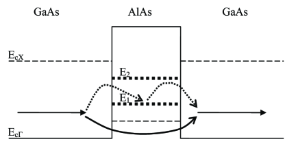
Figure 1: Tunneling through GaAs/AlAs/GaAs barrier. $\Gamma$ band edges are shown by solid line and $X$ band edges are represented by dashed line. $E_{1}$ and $E_{2}$ are $X$-valley quasi-bound states in the AlAs barrier. Direct tunneling ($\Gamma$-$\Gamma$-$\Gamma$) is shown by solid curly arrow and $\Gamma$ -$X$-$\Gamma$ tunneling is depicted by dotted curly arrow.

Spin dependent tunneling has been recently analyzed with a 1-band envelope-function model. Mishra et al. (2005) In their study,Mishra et al. (2005) the authors neglected the ($\Gamma$-$\Gamma$-$\Gamma$) tunneling and the presence of $X$-valley quasi-bound states in the AlAs barrier. However, spin tunneling through the indirect barrier of the GaAs/AlAs/GaAs heterostructure shows another peculiar property. The confined $X$ states in the AlAs barrier interactBeresford et al. (1989) with the continuum $\Gamma$ states in GaAs forming Fano resonancesFano (1961) (i.e.:pairs of resonances/anti-resonances). In this paper we demonstrate that one can use the proximity in the resonance and anti-resonance states in conjunction with the spin splitting produced by the spin-dependent Hamiltonian to obtain a large degree of spin polarization within the range between the resonance and anti-resonance energy. For this purpose we devise a spin-dependent tight-binding model that provides a realistic view of the spin-dependent tunneling through an indirect barrier. We convert the spin-dependent effective mass Hamiltonians for a single band to their tight-binding versions following the recipes of Ref. Frensley, 1994. The coupling between $\Gamma$ and X valleys is made according to Ref. Fu et al., 1993.

The paper is organized as follows. In next section a simple model is analyzed in order to gain insight into the physics of spin-dependent tunneling. The third section contains a realistic tight-binding model and the numerical results. Conclusions are drawn in the fourth section.

II Tight-binding model of spin-dependent tunneling

Consider a simple tight-binding (TB) model of the spin-dependent tunneling through an indirect barrier. The main assumptions for this TB model are: spin states are degenerate in left/right lead (bulk-like states) and the Dresselhaus Hamiltonians are proportional for $\Gamma$ and X states in the barrier, so we can assume that the spin states in the leads are eigenvalues of the Dresselhaus Hamiltonian.

Spin tunneling through an indirect barrier.

The Hamiltonian of the system is

$$\begin{array}[]{l}H=\sum\limits_{n=-\infty,\sigma=\uparrow,\downarrow}^{-1}{\left[{\varepsilon{\kern 1.0pt}c_{n,\sigma}^{+}c_{n,\sigma}+\left({t\,c_{n-1,\sigma}^{+}c_{n,\sigma}+h.c.}\right)}\right]}+\\ \quad\quad\sum\limits_{n=1,\sigma=\uparrow,\downarrow}^{\infty}{\left[{\varepsilon{\kern 1.0pt}c_{n,\sigma}^{+}c_{n,\sigma}+\left({t\,c_{n,\sigma}^{+}c_{n+1,\sigma}+h.c.}\right)}\right]}+\\ \quad\quad\varepsilon_{1}c_{0,\uparrow}^{+}c_{0,\uparrow}+\varepsilon_{2}c_{0,\downarrow}^{+}c_{0,\downarrow}+\left({V_{1}c_{0,\uparrow}^{+}c_{-1,\uparrow}+V_{2}c_{0,\downarrow}^{+}c_{-1,\downarrow}+h.c.}\right)+\\ \quad\quad\left({V_{1}c_{0,\uparrow}^{+}c_{1,\uparrow}+V_{2}c_{0,\downarrow}^{+}c_{1,\downarrow}+h.c.}\right)+\left({t_{1}c_{-1,\uparrow}^{+}c_{1,\uparrow}+t_{2}c_{-1,\downarrow}^{+}c_{1,\downarrow}+h.c.}\right)\\ \end{array}.$$ (5)

The first two terms on the right hand side of Eq. (5) are the Hamiltonians of the contacts (leads), where $\varepsilon$ and $t$ are the on-site energy and transfer integral, respectively (spin degenerate ). $c_{n\sigma}^{+}/c_{n\sigma}$ is the creation/annihilation of an electron with spin $\sigma$ on site $n$. The remaining part is the Hamiltonian of the barrier and its coupling to the leads. The active region is modeled by three sites: site $-1$ that is like the left hand side contact, site $0$ that is the actual barrier, and site $1$ that is like the right hand side contact. Thus the effective left/right hand side contact ends/starts at site $-2/2$. The matrix form of the Hamiltonian for the sites -1, 0, and 1 (in fact $E-H$, where $E$ is energy) with appropriate boundary conditions for an open system isDatta (1995)

$$E-H={\begin{array}[]{*{20}c}\hfill\hfil&{-1\uparrow\hfill}&{-1\downarrow\hfill}&{0\uparrow\hfill}&{0\downarrow\hfill}&{1\uparrow\hfill}&{1\downarrow\hfill}\\ {-1\uparrow\hfill}&{E-\varepsilon-\Sigma_{L}\left(E\right)\hfill}&0\hfill&{-V_{1}\hfill}&0\hfill&{-t_{1}\hfill}&0\hfill\\ {-1\downarrow\hfill}&0\hfill&{E-\varepsilon-\Sigma_{L}\left(E\right)\hfill}&0\hfill&{-V_{2}\hfill}&0\hfill&{-t_{2}\hfill}\\ {\quad 0\uparrow\hfill}&{-V_{1}^{\ast}\hfill}&0\hfill&{E-\varepsilon_{1}\hfill}&0\hfill&{-V_{1}^{\ast}\hfill}&0\hfill\\ {\quad 0\downarrow\hfill}&0\hfill&{-V_{2}^{\ast}\hfill}&0\hfill&{E-\varepsilon_{2}\hfill}&0\hfill&{-V_{2}^{\ast}\hfill}\\ {\quad 1\uparrow\hfill}&{-t_{1}^{\ast}\hfill}&0\hfill&{-V_{1}\hfill}&0\hfill&{E-\varepsilon-\Sigma_{R}\left(E\right)\hfill}&0\hfill\\ {\quad 1\downarrow\hfill}&0\hfill&{-t_{2}^{\ast}\hfill}&0\hfill&{-V_{2}\hfill}&0\hfill&{E-\varepsilon-\Sigma_{R}\left(E\right)\hfill}\\ \end{array}}$$ (6)

where $\Sigma_{L,R}\left(E\right)$ are the self-energies of the semi-infinite parts, i.e.,

$$\Sigma_{L,R}\left(E\right)=t^{+}\frac{1}{E-H_{L,R}+i\delta}\,\,t,$$ (7)

where $H_{L,R}$ are the Hamiltonians of the semi-infinite left and right hand sides and $\delta$ is an infinitesimal positive number. The retarded Green function

$$G_{L,R}^{R}\left(E\right)=\frac{1}{E-H_{L,R}+i\delta}$$ (8)

of the left/right hand side semi-infinite contact in Eq. (7) is actually the diagonal part $G_{L}^{R}\left(E\right)_{-2,-2}/G_{R}^{R}\left(E\right)_{2,2}$ representing the sites $-2$/2. The expressions of these Green function elements can be found from their equation of motion and the use of the finite difference equation method.Chen et al. (1989) If we consider the parameterization $\varepsilon-E=2{\kern 1.0pt}{\kern 1.0pt}t\,\cos\left({ka}\right)$, with $k$ a complex parameter and $a$ a lattice constant parameter, one obtains the following equation for self-energies,

$$\Sigma_{L,R}=-t\,\,e^{ika}.$$ (9)

Therefore, the Green function $G^{R}$ for the sites -1, 0, and 1 with the boundary conditions for an open system is

$$G^{R}\left(E\right)=\left[{{\begin{array}[]{*{20}c}{-t\,e^{-ika}\hfill}&0\hfill&{-V_{1}\hfill}&0\hfill&{-t_{1}\hfill}&0\hfill\\ 0\hfill&{-t\,e^{-ika}\hfill}&0\hfill&{-V_{2}\hfill}&0\hfill&{-t_{2}\hfill}\\ {-V_{1}^{\ast}\hfill}&0\hfill&{E-\varepsilon_{1}\hfill}&0\hfill&{-V_{1}^{\ast}\hfill}&0\hfill\\ 0\hfill&{-V_{2}^{\ast}\hfill}&0\hfill&{E-\varepsilon_{2}\hfill}&0\hfill&{-V_{2}^{\ast}\hfill}\\ {-t_{1}^{\ast}\hfill}&0\hfill&{-V_{1}\hfill}&0\hfill&{-t\,e^{-ika}\hfill}&0\hfill\\ 0\hfill&{-t_{2}^{\ast}\hfill}&0\hfill&{-V_{2}\hfill}&0\hfill&{-t\,e^{-ika}\hfill}\\ \end{array}}}\right]^{-1}.$$ (10)

We notice that the Hamiltonian is not hermitian due to open boundary conditions. To calculate the transmission probability from site $1$ to $N$ we use the formulaDatta (1995)

$$T\left({E,k_{t}}\right)=\Gamma_{L}\left({E,k_{t}}\right)\left|{G_{1,N}^{R}\left({E,k_{t}}\right)}\right|^{2}\Gamma_{R}\left({E,k_{t}}\right),$$ (11)

with

$$\Gamma_{L,R}\left({E,k_{t}}\right)=i\left[{\Sigma_{L,R}\left({E,k_{t}}\right)-\Sigma_{L,R}^{\ast}\left({E,k_{t}}\right)}\right].$$ (12)

Since the Dresselhaus Hamiltonians are proportional at $\Gamma$ and X points in the barrierDresselhaus (1955); Ivchenko and Pikus (1997) we can solve separately for each spin. The Green function for ’spin up’ is

$$G_{\uparrow}^{R}\left(E\right)=\left[{{\begin{array}[]{*{20}c}{-t\,e^{-ika}\hfill}&{-V_{1}\hfill}&{-t_{1}\hfill}\\ {-V_{1}^{\ast}\hfill}&{E-\varepsilon_{1}\hfill}&{-V_{1}^{\ast}\hfill}\\ {-t_{1}^{\ast}\hfill}&{-V_{1}\hfill}&{-t\,e^{-ika}\hfill}\\ \end{array}}}\right]^{-1}.$$ (13)

A similar equation is obtained for the ’spin down’. The poles of $G^{R}$ are the solutions of the determinant equation

$$\Delta=\left|{{\begin{array}[]{*{20}c}{-t\,e^{-ika}\hfill}&{-V_{1}\hfill}&{-t_{1}\hfill}\\ {-V_{1}^{\ast}\hfill}&{E-\varepsilon_{1}\hfill}&{-V_{1}^{\ast}\hfill}\\ {-t_{1}^{\ast}\hfill}&{-V_{1}\hfill}&{-t\,e^{-ika}\hfill}\\ \end{array}}}\right|=0,$$ (14)

while the zeroes of the transmission are the zeroes of the Green function $\left({G_{\uparrow}^{R}}\right)_{1,3}$ relating the sites -1 and 1,

$$\left({G_{\uparrow}^{R}}\right)_{1,3}\left(E\right)=\frac{\left|{{\begin{array}[]{*{20}c}{-V_{1}\hfill}&{E-\varepsilon_{1}\hfill}\\ {-t_{1}\hfill}&{-V_{1}^{\ast}\hfill}\\ \end{array}}}\right|}{\Delta}=0.$$ (15)

The equation for poles reads

$$\left({E-\varepsilon_{1}}\right)\left[{\left|{t_{1}}\right|^{2}-t^{2}\,e^{-2i\,ka}}\right]=\left|{V_{1}}\right|^{2}\left[{-t_{1}-t_{1}^{*}+2\,t\,e^{-i\,ka}}\right]$$ (16)

and for zeroes

$$\left({E-\varepsilon_{1}}\right)\,t_{1}=-\left|{V_{1}}\right|^{2}.$$ (17)

Since $t$ is basically the conduction band bandwidth and $t_{1}$ and $V_{1}$ are tunneling rates, then $V_{1},t_{1}<<t$, such that the pole is given by

$$E\approx\varepsilon_{1}-2\frac{\left|{V_{1}}\right|^{2}}{t}e^{ika}.$$ (18)

The equation for the zero is

$$E=\varepsilon_{1}-\frac{\left|{V_{1}}\right|^{2}}{t_{1}}.$$ (19)

Table 1: Matrix elements in eV of the nearest neighbor model outlined in Eq.  (5).

	Indirect barrier	RTD-like structure
$t$	1.0	1.0
$V_{1}$	0.05	0.005
$V_{2}$	0.052	0.0052
$t_{1}$	0.05	0.0
$t_{2}$	0.052	0.0
$\varepsilon_{1}$	0.17	0.17
$\varepsilon_{2}$	0.175	0.175

Since we have $V_{1},t_{1}<<t$, the energy separation between the pole and the zero is about $V_{1}^{2}/t_{1}$. The resonances and zeroes occur at slightly different energies for the two spin channels, resulting in a large spin polarization due to the combination of a sharp increase in transmission at resonance followed by an abrupt decrease to zero at anti-resonance. Hence, the energy range of large spin polarization will depend on $V_{1}$ and $t_{1}$ but not on the magnitude of spin splitting. One can notice that the energy separation between resonance and anti-resonance can be increased by decreasing $t_{1}$, i.e., increasing the width of the barrier. In Fig. 2 we illustrate the above arguments with the parameters given in Table 1. We also calculate the spin polarization with the equation

$$P=\frac{T_{\uparrow}-T_{\downarrow}}{T_{\uparrow}+T_{\downarrow}}.$$ (20)

For comparison we also plot the case of the resonance tunneling diode (RTD) configuration. The RTD configuration is made by setting $t_{1}$ and $t_{2}$ to 0. To separate the spin resonances, we also have chosen the values of $V_{1}$ and $V_{2}$ ten times smaller than their values in the indirect-barrier configuration. Fig. 2 shows that the indirect barrier configuration has a clear advantage over the RTD configuration.

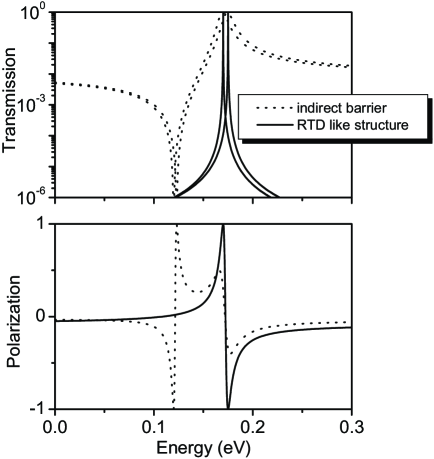
Figure 2: Spin dependent transmission (upper panel) and spin polarization (lower panel) through an indirect barrier versus a resonant tunneling diode configuration. One can see the wide energy window of large polarization created by indirect tunneling.

Spin tunneling through a direct barrier.

Following the same procedure one can also calculate spin transmission through a direct barrier. The Green function of the open system is

$$G^{R}\left(E\right)=\left[{{\begin{array}[]{*{20}c}{-t\,e^{-ika}\hfill}&0\hfill&{-t_{1}\hfill}&0\hfill\\ 0\hfill&{-t\,e^{-ika}\hfill}&0\hfill&{-t_{2}\hfill}\\ {-t_{1}^{\ast}\hfill}&0\hfill&{-t\,e^{-ika}\hfill}&0\hfill\\ 0\hfill&{-t_{1}^{\ast}\hfill}&0\hfill&{-t\,e^{-ika}\hfill}\\ \end{array}}}\right]^{-1}.$$ (21)

The Green function for the ’spin up’ is

$$G_{\uparrow}^{R}\left(E\right)=\left[{{\begin{array}[]{*{20}c}{-t\,e^{-ika}\hfill}&{-t_{1}\hfill}\\ {-t_{1}^{\ast}\hfill}&{-t\,e^{-ika}\hfill}\\ \end{array}}}\right]^{-1}.$$ (22)

Using Eqs. (11) and (12) we calculate the spin-dependent transmission probabilities for a direct barrier. The transmission probabilities are approximated by

$$T_{\uparrow}\approx\frac{4\left|{t_{1}}\right|^{2}}{t^{2}}\sin^{2}{ka}$$ (23)

and

$$T_{\downarrow}\approx\frac{4\left|{t_{2}}\right|^{2}}{t^{2}}\sin^{2}{ka},$$ (24)

i.e., the transmission for ’spin up’ is different from transmission for ’spin down’ leading to spin polarization.

III Results of a realistic tight-binding model and Discussions

In order to make quantitative assessments of the spin tunneling through an indirect barrier, we devise a spin-dependent tight-binding model for a system that is partitioned into layers. The layers from $-\infty$ to $0$ and from $N+1$ to $\infty$ are the contacts, while the layers from $1$ to $N$ are the active layers. First, we consider the spin independent Hamiltonian. The coupling between $\Gamma$ and $X$ states is treated similarly to Ref. Fu et al., 1993, with the Hamiltonian

$$H=\left[{{\begin{array}[]{*{20}c}{H_{\Gamma}\hfill}&{H_{\Gamma X}\hfill}\\ {H_{X\Gamma}\hfill}&{H_{X}\hfill}\\ \end{array}}}\right].$$ (25)

$H_{\Gamma}$ and $H_{X}$ are the Hamiltonians at $\Gamma$ and $X$ point, respectively. $H_{\Gamma{X}}$ and $H_{X\Gamma}$ are the couplings between $\Gamma$ and $X$ at the interface layers. For simplicity, we do not distinguish between $X_{1}$ and $X_{3}$, such that $H_{\Gamma}$ and $H_{X}$ are single-band effective mass Hamiltonians that are converted to TB Hamiltonians according to the parameterization given in Ref. Frensley, 1994. This TB parameterization has been successfully used in quantum transport for non-equilibrium conditions and incoherent scattering processes.Lake et al. (1997) The parameterizationFrensley (1994); Lake et al. (1997) is made for the effective mass Hamiltonian

$$H_{0}=\frac{-\hbar^{2}}{2}\frac{d}{d{\kern 1.0pt}z}\frac{1}{m^{\ast}\left(z\right)}\frac{d}{d{\kern 1.0pt}z}+V_{k}\left(z\right)+\frac{\hbar^{2}k_{t}^{2}}{2{\kern 1.0pt}{\kern 1.0pt}m_{L}^{\ast}},$$ (26)

where $m_{L}^{\ast}$ is the effective mass in the left contact, the effective mass is considered $z$-dependent, and the spatial dependence of the transverse energy has been incorporated in the transverse momentum ($k_{t}$) dependent potential:

$$V_{k}\left(z\right)=V\left(z\right)+\frac{\hbar^{2}k_{t}^{2}}{2m_{L}^{\ast}}\left({\frac{m_{L}^{\ast}}{m\left(z\right)}-1}\right).$$ (27)

The corresponding tight-binding parameters for the non-diagonal part are:

$$t_{ij}=\frac{\hbar^{2}}{\left({m_{i}+m_{j}}\right){\kern 1.0pt}\Delta^{2}}$$ (28)

and the diagonal part is

$$D_{i}\left(k_{t}\right)=\frac{\hbar^{2}}{2{\kern 1.0pt}{\kern 1.0pt}\Delta^{2}}\left({\frac{1}{m^{-}}+\frac{1}{m^{-}}}\right)+V_{i}\left(k_{t}\right).$$ (29)

In Eqs. (28) and  (29), $m_{i}$ is the effective mass at site $i$ on the mesh of spacing $\Delta$, $V_{i}\left(k_{t}\right)$ is the potential at site $i,$ which also includes the band offsets, $m^{-}=\frac{m_{i-1}+m_{i}}{2}$, and $m^{+}=\frac{m_{i}+m_{i+1}}{2}$.

The spin dependent Hamiltonian is expressed in the basis spanned by spinors  (4), such that the Hamiltonian is diagonal in this basis. At $\Gamma$ point the spin dependent part of the effective mass Hamiltonians is introduced through the corrections to the effective masses defined in Eq. (2) and the effective potential defined in Eq. (27). The spin-dependent part at $X$ is expressed through different band offsets for the two spin projections as one can see from Eq. (3).

Table 2: Dresselhaus coefficients at $\Gamma$ and $X$ points for GaAs and AlAs, calculated with the GW methodFaleev et al. (2004); Chantis et al. (2005) with spin-orbit coupling included. The units are the atomic units.

	GaAs	AlAs
$\gamma$	2.1	0.85
$\beta$	0.0074	0.00077

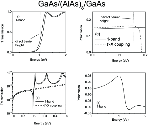
Figure 3: (a) Spin dependent transmission probability of 1-band (direct) tunneling through GaAs/(AlAs)₈/GaAs barrier. (b) Comparison between full (direct and indirect) and 1-band (direct) transmission probability of a GaAs/(AlAs)₈/GaAs barrier. (c) Comparison of spin polarization between full (direct and indirect) and 1-band (direct) electron transmission of a GaAs/(AlAs)₈/GaAs barrier. (d) Spin polarization obtained from 1-band calculation over a broader energy range.

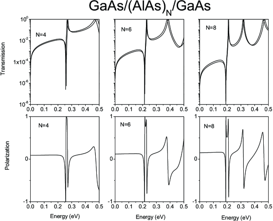
Figure 4: Spin dependent transmission probability and spin polarization of a GaAs/(AlAs)_N/GaAs heterostructure. $N$=4, 6, and 8.

Our calculations are performed with the effective masses and band edges taken from Ref. Klimeck et al., 2000. The Dresselhaus parameters given in Table 2 are calculated with a quasi-particle self-consistent GW (G=Green function, W=screened Coulomb interaction) method as in Ref. Faleev et al., 2004; Chantis et al., 2005 with spin-orbit coupling included perturbatively. The splitting at $\Gamma$ in GaAs found in the present work with the GW method is three times smaller than the value used by Perel et al. in Ref. Perel’ et al., 2003.Pikus et al. (1988) The GW spin splitting at $\Gamma$ for AlAs is about 2.5 times smaller than in GaAs. While for GaAs one can also use the experimental estimation for the splitting at the $\Gamma$ point Pikus et al. (1988) there are no such estimations for AlAs. Therefore to be consistent, we used the GW values for both. The value of spin splitting at $X$ point is almost the same as the one obtained within the local density approximation (LDA) with our FP-LMTO (full potential-linear muffin-tin orbitals) code. Methfessel et al. (2000) The $X$-$\Gamma$ band offset for GaAs/AlAs heterostructure is chosen to be 160 meV.Mendez et al. (1988) Throughout the paper we have chosen a value $k_{t}=\frac{2\pi}{a}\times 0.05$ for the transverse wave vector ($a$ is the lattice constant of GaAs).

In Fig. 3 we compare the one-band model (direct tunneling) given by the effective mass Hamiltonian and the two-band model (direct and indirect tunneling) given by Eq. (25). Below the indirect barrier, the main contribution to spin tunneling and polarization is provided by direct tunneling. However, the tunneling and the polarization through $X$ states become dominant for energies above the indirect barrier. The result shows that the confinement of the $X$ states in the barrier increases the energy threshold at which the tunneling through $X$ states becomes dominant. In the calculationsMishra et al. (2005) in which the confinement of the $X$ states in the barrier are neglected, the tunneling is predominantly indirect for energies slightly below the top of indirect barrier. Therefore, our calculations suggest that multi-band calculations are needed to fully describe the electron transport in these heterostructures.

In Fig. 4 we show the transmission probability and spin polarization for GaAs/(AlAs)_N/GaAs heterostructures with $N$ = 4, 6, and 8. Energy windows with large polarization can be seen between the resonance and its corresponding zero. The width of the window increases with the barrier width as it has been demonstrated in the previous section. Only the first resonance has a corresponding zero on the real axis, for the other resonances, the zeroes are pushed off the real axis.Bowen et al. (1995) Therefore, if the resonances are close enough, no well defined window with large spin polarization can be found. The possibility to obtain well separated resonances with zeroes on the real axis is controlled by the combination of the longitudinal effective mass in the barrier at $X$ point and the barrier width. A lighter longitudinal effective mass and/or a narrower barrier push farther apart the resonance energies in the barrier.

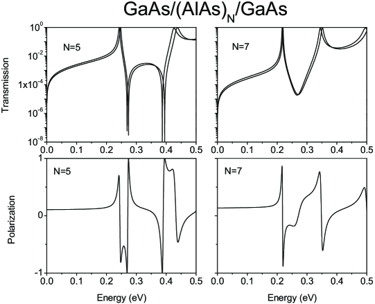
Figure 5: Spin dependent transmission probability and spin polarization of a GaAs/(AlAs)_N/GaAs heterostructure. $N$ = 5 and 7.

In Fig. 5 we plot the transmission probability and spin polarization for GaAs/(AlAs)_N/GaAs with $N$ = 5 and 7. The parity of the number of AlAs monolayers has been taken into account. Fu et al. (1993) The case $N$= 5 shows two wide windows with large and opposite spin polarizations. Again, the polarization windows are mainly determined by the resonance and anti-resonance positions and not by the magnitude of spin splitting. However, $N$ = 7 shows no such energy windows because the zeroes have moved away from the real axis. Moreover, at larger values of $N$ no energy windows with large polarization are found for both even and odd values of $N$.

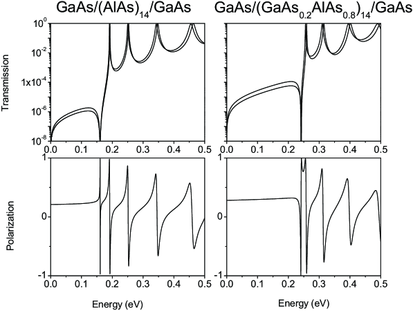
Figure 6: Comparison of spin dependent transmission probability and spin polarization between GaAs/(AlAs)₁₂/GaAs and GaAs/(Al_0.8Ga_0.2As)₁₂/GaAs heterostructures.

The pattern can be re-established by increasing the strength of the Dresselhaus coefficient at $X$ point in the barrier. A barrier made of Al_0.8Ga_0.2As can achieve this goal. In Al_0.8Ga_0.2As, the Dresselhaus coefficients are mixtures of those of AlAs and GaAs. GaAs has larger coefficients, in particular, $\beta$ is ten times larger than the $\beta$ coefficient of AlAs, making the $\beta$ coefficient of the compound stronger than that of AlAs. In Fig. 6 we make a comparison between Al_0.8Ga_0.2As and AlAs barriers with a thickness of $N$=12 monolayers. Virtual crystal approximation was employed to calculate the physical parameters of Al_0.8Ga_0.2As. This is a reasonable assumption, since AlAs and GaAs have similar structural and electronic properties. Fig. 6 illustrates clearly that Al_0.8Ga_0.2As barrier shows a window of polarization, while AlAs barrier does not.

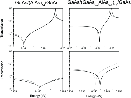
Figure 7: Closer look at spin dependent transmission probability around resonance energy for GaAs/(AlAs)₁₂/GaAs and GaAs/(Al_0.8Ga_0.2As)₁₂/GaAs heterostructures. It explains the origin of energy window with large spin polarization.

Visual analysis of Fig. 6 and Fig. 7 suggests that in order to obtain polarization windows, the resonances and zeroes in the spin channels must be properly ordered. If a resonance is occurring first in the spin channel 1, the zero in the transmission coefficient of the spin channel 1 must precede the zero in the transmission coefficient of spin channel 2. This condition is fulfilled for wider barriers provided that the Dresselhaus coefficient at $X$ point is sufficiently large.

The practical aspect of focusing the electrons to energies within the large-polarization window can be achieved by placing an RTD structure in front of the tunneling barrier. In this way, one not only can control the incoming energy of the electrons but also ensures that most electrons have non-vanishing transverse momentaSandu et al. (2003) and, consequently, their energies are spin-split.

It is important to analyze at this point the influence that the neglect of the Dresselhaus $k^{3}$ term in the leads can have on the conclusions drawn in the present work. Since the tight-binding basis is localized, different basis can be used to treat the spin Hamiltonian in barrier and in the leads. In the leads, the basis is that which makes diagonal the Hamiltonian in Eq. (2), while in the barrier the basis is given in Eq. (4). The non-diagonal spin dependent part is then transferred to interface terms between leads and barrier. The corrections to the Green function and transmission coefficients are quadratic with respect the strength of this non-diagonal term. This analysis indicates that the conclusions of the article are not likely to change if the Dresselhaus term in the leads is properly taken into account. A detailed quantitative discussion will be presented elsewhere since special care must be exercised due to the presence of the $k_{z}$-linear term in Eq. (2).

IV Conclusions

We investigated the spin dependent transport across an indirect semiconductor barrier of a zinc-blende structure like GaAs/AlAs/GaAs heterostructure along [001] axis by means of a combination of several tight-binding models. Spin tunneling through such an indirect barrier exhibits two major characteristics: the proportionality of the Dresselhaus Hamiltonians at $\Gamma$ and $X$ points and the Fano resonances. A generic tight-binding Hamiltonian has shown that large spin polarization occurs in the energy window determined by the separation between the resonance and its associated anti-resonance and not by the magnitude of the spin splitting of resonances. Moreover, the energy separation between the resonance and its corresponding anti-resonance increases as the barrier width increases.

Realistic calculations have been performed with a two-band tight-binding model. The effective mass Hamiltonians at $\Gamma$ and $X$ have been convertedFrensley (1994) to the tight-binding Hamiltonians. The $\Gamma$-$X$ coupling was implemented following the scheme presented in Ref. Fu et al., 1993. Accordingly, the Dresselhaus Hamiltonians at $\Gamma$ and $X$ in the barrier have been included in the effective masses and band offsets. The calculations show that, in order to obtain energy windows with large polarization, two conditions need to be satisfied. The first condition consists of having well separated resonances such that their corresponding anti-resonances do not interact with each other. The second condition is that the relative energy order of the resonances in the two spin channels must be the same as the order of their corresponding zeroes. The first condition is achieved by an appropriate combination of barrier width and longitudinal effective mass at $X$ point, while the second condition is accomplished by a combination of spin splitting strength at $X$ point and transmissibility through the direct barrier.

Electrons can be focused in the required energy windows by passing them through a resonant tunneling diode structure situated in front of the indirect barrier. Using such an experimental setup, one could obtain large spin polarization following the procedure of Perel et al.Perel’ et al. (2003) and Glazov et al.Glazov et al. (2005).