Low-loss resonant modes in deterministically aperiodic nanopillar waveguides

Abstract

Quasiperiodic Fibonacci-like and fractal Cantor-like single- and multiple-row nanopillar waveguides are investigated theoretically employing the finite difference time domain (FDTD) method. It is shown that resonant modes of the Fibonacci and Cantor waveguides can have a Q-factor comparable with that of a point-defect resonator embedded in a periodic nanopillar waveguide, while the radiation is preferably emitted into the waveguide direction, thus improving coupling to an unstructured dielectric waveguide located along the structure axis. This is especially so when the dielectric waveguide introduces a small perturbation in the aperiodic structure, breaking the structure symmetry while staying well apart from the main localization area of the resonant mode. The high Q-factor and increased coupling with external dielectric waveguide suggest using the proposed deterministically aperiodic nanopillar waveguides in photonic integrated circuits.

I Introduction

In the recent decade, defects in two-dimensional (2D) photonic crystals have been widely considered for use as photonic microcavities jmwBook ; sakodaBook . A substantial amount of work has been devoted to optimizing the Q-factor of the resonant mode while maintaining the small mode volume (see Recipe and references therein). Since a 2D photonic crystal does not possess a complete 3D photonic band gap, numerous efforts were dedicated to determining the influence of cladding or substrate on the resonator quality Deloc1 ; Deloc2 . There have been efforts to utilize resonant modes in a 2D system for microlasers Deloc2 ; IEICE and to employ the resonant mode formalism in random lasing studies cao05 ; Deloc3 .

As it has recently been discussed, periodic one-dimensional (1D) arrangement of dielectric nanopillars (nanopillar waveguides) can support guided modes Fan95 ; AVL ; AVL2 . Such a dielectric structured waveguides possess good light confinement along with the strongly modified dispersion. The current state-of-the-art fabrication technologies makes practical realization of the nanopillar structures feasible. To ensure the vertical light confinement and low losses, the pillar-based dielectric structures can be realized both in sandwich-like geometry pillar04 ; pillar05 and in membrane-like geometry ParkLee . Along with known studies of lasing in single nanowires and nanowires arrays Lasing , it is suggested that nanopillar geometry, and in particular 1D nanopillar arrangements, can prove a good alternative to already known 1D and 2D microstructured waveguides and integrated optical devices based on them.

Most applications involve introducing a defect into a waveguide-like structure, e.g. for use as a microresonator, coupled to a 1D waveguide as an input or output terminal. Usually, the defect is considered to be point-like, created by altering the properties of one or several adjacent nanopillars (see, e.g., Fig. 1a) Fan95 ; Johnson . However, due to the absence of a complete band gap, the breaking of translational symmetry caused by the defect inevitably results in radiation losses of the microresonator mode by coupling to the surrounding electromagnetic continuum. The losses should be much stronger in the case of 1D nanopillar waveguides than in the more studied case of 2D periodic structures. This raises the need for optimizing the Q-factor of the resonator in 1D nanopillar waveguides. If one were to couple the resonant mode efficiently to an external unstructured dielectric waveguide, located along the nanopillar waveguide axis, and if the amount of energy escaping through this dielectric waveguide were greater than that leaving the resonator elsewhere, this would prove useful in many design aspects of nanosized optical components, for instance microlaser resonators.

There have been some proposals to decrease the losses based on either mode delocalization Deloc1 or on the effect of multipole cancellation Johnson . However, a delocalized mode typically suffers from a decrease of the Q-factor. On the other hand, the spatial radiation loss profile of a mode described in Johnson has a nodal line along the waveguide axis, which means poor coupling to any components coaxial with the waveguide.

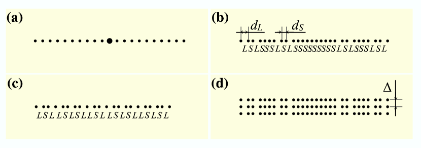
Figure 1: Top view of a point-defect periodic reference waveguide (a), a third-generation Cantor nanopillar waveguide (b), a 7-stage Fibonacci waveguide (c), and a three-row Cantor waveguide with row spacing $\Delta=0.75a$ (d). Black circles correspond to cylinders with $\varepsilon=13.0$, extending infinitely in the third dimension and located in air. For the FDTD calculations a spatial grid with 16 mesh points per unit length $a$ was used. The whole area of computation is a $7a\times 22a$ rectangle surrounded by PML boundaries, see section II.1 for details.

Other than by means of a point defect, a resonant system can also be created by changing the periodic arrangement of nanopillars into non-periodic. There is a wide variety of possibilities for creating such a deterministically aperiodic structure. The most studies cases of such structures are quasiperiodic (e.g. Fibonacci-like) Kohmoto and fractal (e.g. Cantor-like) PRE structures. The examples are shown in Fig. 1b,c. In a 1D multilayer model, such deterministically aperiodic structures are known to support eigenmodes which are highly localized yet with the localization character different from exponential Kohmoto , as well as with localization patterns extending over several similar defects throughout the structure PRE . In addition, several of such non-periodic waveguides can easily be aligned next to each other to form a multi-row nanopillar waveguide (see Fig. 1d) AVL ; AVL2 . It causes waveguide modes to split, as it always happens when several resonant systems are coupled. What is more, each of these split modes can be selectively excited if the excitation pattern resembles the profile of the corresponding mode AVL .

In this paper, we investigate the resonant modes in single- and multi-row nanopillar waveguides constructed according to two known deterministically aperiodic sequences – a quasiperiodic Fibonacci Primer and a middle-third Cantor fractal sequence EPL – and compare their properties to those of the resonant modes of a point-defect reference system Johnson . We show that, although the resonant modes of a point defect generally exhibit a higher Q-factor and always have a smaller mode volume, in a 1D periodic nanopillar arrangement the coupling to an external terminal (a semi-infinite rectangular unstructured waveguide placed coaxially with nanopillar waveguide) is poor, unless the terminal is brought very close to the defect. On the contrary, both in a Fibonacci and in a Cantor waveguide there is a good coupling to the terminal while maintaining a high Q-factor. The coupling increases even further when the terminal breaks the symmetry of the Fibonacci or Cantor structure, yet stays well apart from the mode’s main localization region. Both the Q-factor and the coupling are found to improve even further if multiple-row Cantor nanopillar waveguides are used.

The paper is organized as follows. In Section II we describe the construction of quasiperiodic and fractal nanopillar waveguides. The analysis of the resonant modes Q-factors is presented for single- and multiple-row deterministic aperiodic waveguides. In Section III we discuss the coupling of resonant modes with an external unstructured dielectric waveguide and show a distinct advantage in both Cantor and Fibonacci cases over a reference point-defect system. In Section IV the multiple-row Cantor waveguides are studied. Finally, Section V summarizes the paper.

II Resonant modes in aperiodic waveguides

II.1 Generation of aperiodic structures and computational method

As a system under study, we have chosen a non-periodic 1D array of cylindrical nanopillars of equal diameter, the distances between adjacent pillars given by Fibonacci and Cantor sequences, respectively. If we denote $S$ and $L$ for short and long distance ($d_{S}$ and $d_{L}$), respectively, the Fibonacci sequence is constructed by the inflation rule,

$$L\to LS,\quad S\to L,$$ (1)

and reads,

$$L \to LS\to LSL\to LSL\,LS$$

$$\to LSLLS\,LSL\to LSLLSLSL\,LSLLS\to\cdots\ .$$

The Cantor sequence is created by the inflation rule

$$L\to LSL,\quad S\to SSS.$$ (3)

and unfolds in the following self-similar fashion, which represents a series of middle third Cantor prefractals

$$L \to LSL\to LSL\,SSS\,LSL$$

$$\to LSLSSSLSL\,SSSSSSSSS\,LSLSSSLSL\to\cdots.$$

For the Fibonacci sequence, it is remarkable that the distance from the first pillar (which has number $0$) to the $n$th pillar can be expressed via the simple, explicit relation Primer ,

$$d(n)=d_{S}n+\left(d_{L}-d_{S}\right)\left\lfloor\frac{n-1}{\tau}\right\rfloor,$$ (5)

$\tau=(1+\sqrt{5})/2$ being the golden mean. We have found that a similar formula for a Cantor sequence can be derived, albeit considerably more complicated,

$$d(n)=d_{S}n+\left(d_{L}-d_{S}\right)\sum_{j=1}^{n}\prod_{k=1}^{\left\lceil N\right\rceil}\left(1-2\left\{\frac{1}{2}\left\lfloor\frac{j-1}{3^{k}}\right\rfloor\right\}\right).$$ (6)

In Eqs. (5–6), the expressions $\left\lfloor x\right\rfloor$, $\left\lceil x\right\rceil$, and $\left\{x\right\}$ denote floor integer, ceiling integer, and fractional parts of $x$, respectively, whereas $N=\log_{3}n$. For the realizations of our aperiodic structures we have chosen for the radius of a nanopillar $r=0.15a$ and for the short and long spacings between adjacent nanopillars $d_{S}=0.5a$ and $d_{L}=0.81a$, respectively. The pillars have a dielectric constant $\varepsilon=13$ and are placed in air ($\varepsilon=1$). Fig. 1 shows a “top view” of a 3rd-generation Cantor structure consisting of $28$ nanopillars (Fig. 1b) as well as a 7th-stage Fibonacci structure consisting of $22$ nanopillars (Fig. 1c). The pillars are arranged according to Eqs. (6) and (5), respectively. Three-row Cantor and Fibonacci structures were made by putting 3 single-row structures in parallel at a distance $\Delta$. Fig. 1d shows a 3-row Cantor structure for $\Delta=0.75a$. As a reference system (also called point-defect system in what follows), we consider a periodic array of the same nanopillars (spacing $d_{L}$) with a point defect in the middleJohnson (Fig. 1a). In analogy to 1D multilayer structures PRE , we have chosen a defect with the highest Q-factor possible, given a fixed number of pillars or layers. The defect is created by doubling the radius of one of the nanopillars. This is advantageous over, say, eliminating one pillar or reducing its radius, because the defect mode is mostly localized within the optically dense medium, thus reducing radiation losses.

The temporal evolution of fields in these systems was calculated using the 2D finite difference time domain (FDTD) methodFDTD . The waveguide was placed inside a computation area, which is a $7a\times 22a$ rectangle, with 16 mesh points per unit length $a$. In order to simulate radiation boundary conditions, perfectly matched layer (PML), which is designed to absorb all outgoing radiation without any reflection PML , surrounded the rectangular computation area.

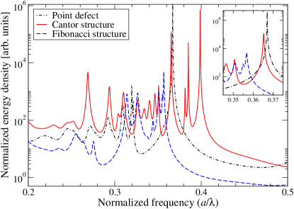
Figure 2: Normalized energy density spectra of a Cantor (Fig. 1b) and Fibonacci (Fig. 1c) waveguide versus a point-defect reference waveguide (Fig. 1a). The inset shows the resonance peaks under study, located in the vicinity of the point defect resonance.

To determine the spectral response of our systems, they were excited by point dipole sources with random phase $\phi(\mathbf{r})$, so that at each point within the excitation area there is a current

$$\mathbf{j}(\mathbf{r},t)=-i\omega_{0}\mathbf{d}\delta(\mathbf{r})e^{-i(\omega_{0}t+\phi(\mathbf{r}))}e^{-\frac{(t-t_{0})^{2}}{\sigma}}.$$ (7)

Evidently, this source is a Gaussian pulse (half width $\sqrt{\sigma}$) of a dipole with base frequency $\omega_{0}$. The pulse was introduced to make such sources emit a signal with a broad spectrum rather than the $\delta$-function spectrum of a purely harmonic dipole source, where $1/\sqrt{\sigma}$ was chosen large enough to cover the frequency window of interest. The spectral dependence of the energy density inside the system was then obtained using Fourier transformation. The phase function $\phi(\mathbf{r})$ in Eq. (7) is taken to be random, and the calculation was repeated with subsequent averaging over several realizations. This is necessary in order to uniformly excite all possible modes in the system.

Table 1: Normalized peak frequencies and corresponding Q-factors of some resonant modes for single- and multiple-row nanopillar structures similar to those shown in Fig. 1.

Fig.	Structure	$a/\lambda$	Q-factor
1a	Reference	0.367	$2.1\times 10^{4}$
1b	Cantor	0.365	$2.7\times 10^{3}$
1c	Fibonacci	0.357	$0.95\times 10^{3}$
1d	3-row Cantor, $\Delta=0.75a$	0.353	$1.1\times 10^{4}$
		0.376	$2.4\times 10^{4}$
	3-row Cantor, $\Delta=a$	0.360	$1.1\times 10^{4}$
		0.370	$1.6\times 10^{4}$
	3-row Fibonacci, $\Delta=0.75a$	0.343	$1.1\times 10^{3}$
		0.356	$1.1\times 10^{3}$
		0.366	$1.6\times 10^{3}$
		0.373	$1.7\times 10^{3}$

II.2 Spectral response and resonant modes

We now investigate the resonant modes in isolated, deterministically aperiodic waveguides, i.e., without coupling to an external terminal, in order to justify that those resonant states can compete with “traditional” defect states in terms of their Q-factor. The spectra for Cantor and Fibonacci waveguides vs. reference system, normalized to the spectral response of free space to eliminate the influence of the sources, are shown in Fig. 2. One can see that the reference system has a band gap above the normalized frequency $a/\lambda=0.32$, where $\lambda$ is the vacuum wavelength. In addition, the system exhibits a single sharp peak inside the band gap at $a/\lambda\approx 0.365$, which is obviously associated with the defect. The Cantor waveguide does not exhibit a true band edge, but instead a crossover from the continuous spectrum (where the spectrum contains long-wavelength, effective-medium extended modes) to the fractal part of the spectrum (which primarily consists of resonant states intermingled with local band pseudogaps) fractons . This crossover happens at a certain frequency (the phonon-fracton crossover frequency) found around $a/\lambda\approx 0.346$. The Cantor structure also exhibits a resonance peak very close to the resonance of the reference system. Since it is located above the phonon-fracton crossover, it is also associated with distortions with respect to a periodic lattice. For the Fibonacci waveguide there is a group of peaks which form a transmission band within a local pseudogap above $a/\lambda=0.3$. All structures in question exhibit resonant modes at frequencies very near to each other, which makes these modes suitable for comparative studies. Three-row waveguides tend to have richer peak spectra resulting from the splitting (not shown here). However, several relatively isolated resonance peaks can usually be found in the region of interest.

To estimate the resonant mode Q-factor, the system is excited by a single point dipole oscillating harmonically at the resonant frequency. After stationary oscillations were achieved, the dipole source was slowly turned off, and after that the subsequent field–time dependencies were analyzed in order to determine the mode Q-factor as

$$Q=\frac{\omega\Delta t}{\alpha},\quad\alpha\equiv-\frac{d}{dj}\log\left\langle\left|\mathbf{E}(j)\right|\right\rangle\ ,$$ (8)

where $\mathbf{E}$ is the electric field, $\langle\dots\rangle$ denotes the average over sufficiently many time steps $j$ so as to include a lot of light oscillations, and $\Delta t$ is the time step width. The results are compiled in Table 1.

One can see that for a single-row Cantor waveguide the resonant mode Q-factor is about one order of magnitude less than that for the point defect. Various peaks within the above-mentioned Fibonacci pass band generally have a Q-factor a couple of times less than that for Cantor structure. As shown in Table 1, in the three-row Cantor waveguides the Q-factor is seen to rise to higher values and becomes comparable to that of a point-defect reference waveguide. It is not the case, however, in multi-row Fibonacci waveguides where resonant modes exhibit only a moderate increase of the Q-factor.

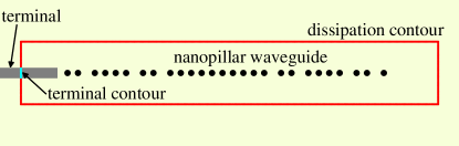
Figure 3: The numerical set-up for energy flux calculations. The rectangular closed contour is divided into a “dissipation part” outside the terminal (red) and the “terminal part” inside (cyan). The waveguide shown here is a Cantor structure with leftmost nanopillar removed. The terminal width is $0.5a$.

III Coupling to an external terminal

In the previous section we have shown that deterministic aperiodic waveguides possess a Q-factor at least comparable to that of a point-defect resonator. In this section, we demonstrate that Fibonacci and Cantor waveguides can be more preferable in applications involving the energy exchange between the resonant system and the outside world in a controlled way. By that we mean, that the balance between the “useful radiation", i.e., radiation directed into the coaxial terminal, and the “lost radiation", i.e., radiation directed out of the waveguide axis, can be considerably shifted in favor of the “useful radiation" in the case of proposed aperiodic structures without a dramatic compromise to Q-factor.

The terminal introduced here is an unstructured dielectric rectangular waveguide coaxial with the nanopillar waveguide and positioned at one of its ends. Since the terminal goes all the way into the PML boundary layer, it can be considered semi-infinite from the point of view of our model. To determine the spectral energy exchange characteristics of the system, we place a single Gaussian-pulse point dipole source, as described by Eq. (7), in the center of the structure and analyze the Poynting vector $\mathbf{S}$ associated with the electromagnetic fields $\mathbf{E}$ and $\mathbf{H}$ at frequency $\omega$, averaged over time, i.e.

$$\overline{\mathbf{S}(\omega,\mathbf{r})} = \int_{0}^{2\pi/\omega}\frac{\omega\,dt}{2\pi}\left|\mathbf{E}(\omega,\mathbf{r})\times\mathbf{H}(\omega,\mathbf{r})\cos^{2}(\omega t)\right|$$ (9)

$$= \frac{1}{2}\textrm{Re}[\mathbf{E}(\omega,\mathbf{r})\times\mathbf{H}^{*}(\omega,\mathbf{r})].$$

Since our computational scheme is effectively two-dimensional, the total energy flux at frequency $\omega$ is an integral over a contour enclosing the waveguide structure. If the contour contains no structure, the energy flux takes the form

$$S_{0}(\omega)\equiv\oint\overline{\mathbf{S}_{0}(\omega,\mathbf{r})}\cdot\mathbf{n}dl\sim\frac{\sigma}{2}\omega\omega_{0}^{2}e^{-\frac{\sigma}{2}(\omega-\omega_{0})^{2}},$$ (10)

naturally independent of the closed contour shape. For computational simplicity, it was chosen to be rectangular, as shown in Fig. 3. Equation 10 has been confirmed by numerical calculations.

For a source radiating into the empty space the energy flux is isotropic, so the flux $S_{f}$ through any contour fragment carries the same frequency dependence as in Eq. 10, attenuated proportional to the aperture angle of that fragment $\theta_{f}/2\pi$.

As soon as a nanopillar structure supporting resonant modes is placed inside the contour, with as well as without the terminal, a strong redistribution of energy flux takes place. This redistribution is both spectral and spatial. The spectral one is seen as peaks at resonant frequencies, where energy is stored within the structure for a dwell time given by the inverse resonance width. The spatial redistribution accounts for the pattern according to which the energy is radiated. In order to quantify the amount of energy directed into the terminal compared to the amount of energy lost by radiation into the continuous modes of the surrounding homogenous medium (e.g. air), we break our closed contour into a “terminal part”, spanning the cross-section of the terminal, and a “dissipation part” elsewhere (see Fig. 3). The contour integrals of $\overline{\mathbf{S}(\omega,\mathbf{r})}$ along these two fragments are named terminal and dissipative fluxes, $S_{t}(\omega)$ and $S_{d}(\omega)$, respectively. The flux ratio

$$\eta(\omega)\equiv S_{t}(\omega)/S_{d}(\omega)$$ (11)

is then a quantitative measure of the balance between "usefull" and "lost" radiated power. For device applications involving a microresonator mode coupled to an optical circuit both $\eta$ and $Q$ should be maximized. If we are to characterize the resonant modes themselves with respect to spatial energy redistribution, independent of the aperture of the terminal, it is useful to compare the angular flux densities, i.e. the fluxes $S_{t}$ and $S_{d}$ devided by their respective aperture angles $\theta_{t}$ and $\theta_{d}$, as seen from the source position. In this way one obtains the flux density ratio

$$\zeta(\omega)\equiv S_{t}(\omega)\,\theta_{d}/S_{d}(\omega)\,\theta_{t}.$$ (12)

To eliminate the influence of the source spectrum on $S_{t}(\omega)$ and $S_{d}(\omega)$, one can normalize the energy fluxes by $S_{0}(\omega)$, Eq. (10).

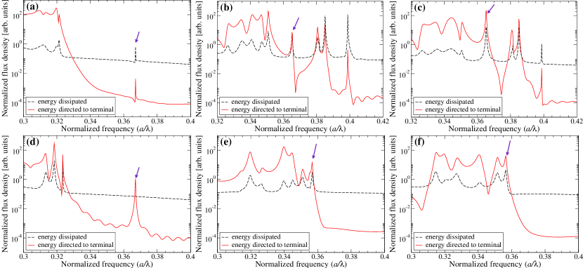
Figure 4: The spectral energy flux densities, normalized to the total spectral flux $S_{0}(\omega)$, through the terminal, $S_{t}(\omega)/\theta_{t}$, (red solid line) and elsewhere, $S_{d}(\omega)/\theta_{d}$, (black dashed line) for the reference point-defect structure (a), a Cantor waveguide without (b) and with (c) structure symmetry breaking, and a Fibonacci waveguide without (e) and with (f) structure symmetry breaking. The plot (d) corresponds to a point defect located 3 nanopillars away from the terminal.

The results of numerical calculations are depicted in Fig. 4. We can see at once that in a band gap the energy is mainly scattered out of the nanopillar waveguide, with $S_{t}$ less than $S_{d}$ by 4-5 orders of magnitude. This is the case for all structures under study. Taking into account the ratio of aperture angles, which in our setup equals $0.00898$ (so roughly $\zeta\approx 100\eta$), one sees that $\zeta\simeq 10^{-2}\ldots 10^{-3}$. This is so because a structure with a band gap cannot function as a waveguide, prohibiting wave propagation in the direction of its axis and thus radiating the energy mostly into the other directions. On the other hand, in the pass band of a waveguide (especially in the case of the reference system, Fig. 4a), the energy directed into the terminal can approach or even exceed the energy radiated elsewhere, so that $\eta\simeq 1$ and $\zeta\simeq 10^{2}$. This is quite natural because the corresponding modes are extended and, thus, have a very good coupling to the terminal. However, it also means inevitably a low Q-factor. Looking at the defect mode in the reference system (Fig. 4a), we can see that although there is a peak in both energy fluxes, the terminal flux is nearly as marginal compared to the dissipative flux as in the gap ($\eta\approx 10^{-2}$). This means that, although this defect mode has a high Q-factor, most of the energy is radiated in the transverse derections.

For the Cantor waveguides the situation is different. As seen from Fig. 4b, for the resonant peak identified in Table 1, a considerable fraction of energy is directed into the terminal, the ratio $\zeta$ being around $1$. Off-peak, $\zeta$ decreases substantially, which identifies the peak as corresponding to a resonant mode. For the Fibonacci waveguide (Fig. 4e), the group of peaks in Fig. 2 generally resembles a pass-band bahavior, but with a lower $\zeta\approx 1\,\dots\,10$, with the slight exception for the two rightmost peaks. However, the Q-factor of these peaks is diminished (c.f. Table 1) due to the proximity to the pass band and due to a more extended nature of the Fibonacci eigenstates.

For both Cantor and Fibonacci waveguides, the coupling can be improved further, if the nanopillar closest to the terminal is removed from the waveguide and the terminal is extended accordingly to keep the terminal–waveguide distance unchanged (for the Cantor structure, compare Fig. 1b with Fig. 3). In this case the internal symmetry of the structure, as implied by Eqs. (II.1) and (II.1), becomes distorted. Looking at Figs. 4c and 4f for Cantor and Fibonacci waveguides, respectively, one can see that for the $a/\lambda=0.365$ resonance, $\zeta$ can amount on-peak to $10$ while off-peak it is still far below $1$. This means that a substantial part of resonant mode energy is coupled into the terminal. Such a situation does not occur for all peaks, however. For example, the low-Q, pass-band states for $a/\lambda\lesssim 0.36$ as well as the resonance at $a/\lambda\approx 0.4$ for Cantor structures retain their behavior as in the structure with unbroken symmetry.

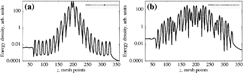
Figure 5: The energy density profile along the longitudinal waveguide axis for the reference point-defect (a) and Cantor (b) systems respectively. The corresponding structures are shown as insets. The terminal is located to the left of each structure.

Let us point out for comparison that altering the point-defect waveguide (Fig. 1a) in a like manner, i.e., removing its leftmost pillar, does not change the coupling efficiency. Only by moving the defect as close as $3$ pillars away from the terminal increases the coupling to comparable values with the Cantor structure case (see Fig. 4d). However, this symmetry breaking is accompanied by a drop in Q-factor by as much as two orders of magnitude, while removing one pillar from aperiodic (Cantor or Fibonacci) waveguides causes only a 10% decrease.

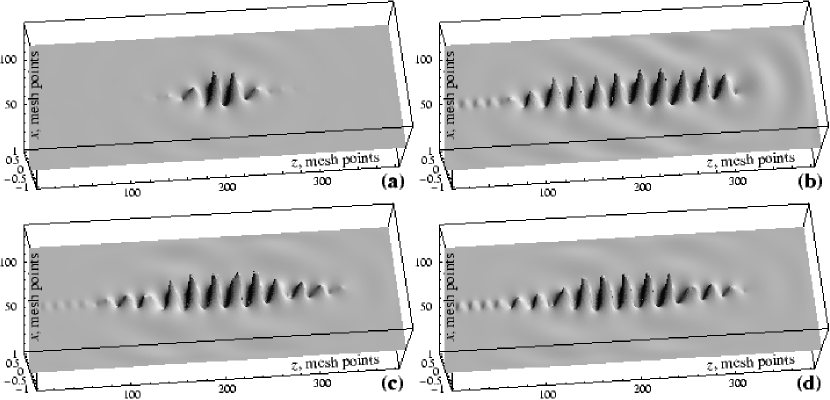
Figure 6: Electric field distributions, normalized to their respective maximum values, for the resonant modes under study in presence of an external terminal: in the reference point defect structure as seen in Fig. 1a (a); in the Fibonacci (b) and Cantor (c) structure as depicted in Fig. 1b,c; in the same Cantor structure when the terminal in positioned so as to cover the first nanopillar and thus break the structure internal symmetry (d). The system was excited by a single monochromatic dipole source in the center of the structure at the respective resonance frequency.

Now we discuss the origin of the radiated power redistribution in favor of improved coupling to the terminal in the case of aperiodic structures as compared to periodic waveguides with a point defect. Figure 5 shows the energy density in a point defect structure (a) and a Cantor waveguide (b) along the axis of the structure, when excited by a harmonic point defect in the center of the structure. It is seen that in the periodic structure, the defect mode is strongly exponentially localized around the point defect, and due to this exponential character the coupling is very poor. On the other hand, in the Cantor structure the energy density spreads out far more to the ends of the structure, while maintaining a relatively high Q-factor (c.f. Table 1), leading to an enhanced coupling to the terminal and reduced radiation losses in the transverse direction. Note that this is not only due to the increased mode volume, but also because of a difference in mode localization character. We speculate that this is a precursor effect of the, on average, powerlaw localized, critical eigenmodes that are expected for an infinite aperiodic system, in analogy to the critical eigenstates of quasicrystals Primer ; Kohmoto .

To visualize these results, we excited the systems with a monochromatic point dipole at the respective resonant frequencies shown in Table 1 and recorded the resulting electric field distributions. The results are shown in Fig. 6. In the point defect (Fig. 6a), the field is strongly localized with nearly isotropic radiation profile containing a nodal line along the waveguide. Hence, nearly all the energy is dissipated sideways in accordance with Ref. Johnson . For the Cantor structures (Fig. 6c), there is a sizable field amplitude excited inside the terminal. The field in the surrounding area is comparable to that in the terminal, in agreement with Fig. 4b. This behavior is further enhanced when the waveguide is used without its leftmost nanopillar, i.e., if the terminal breaks the structure’s symmetry (Fig. 6d). The amplitude of sideways-directed radiation is the same as in Fig. 6c, but the field inside the terminal is greater, as implied by the condition $\zeta>1$. Figure 6b shows the field distribution for the Fibonacci structure. The resonant mode is less localized and the field inside the terminal is visibly more pronounced than for the Cantor structure (Fig. 6c), but so are sideways-directed radiation, resulting from smaller values of $\zeta$.

IV Multiple-row Cantor waveguides

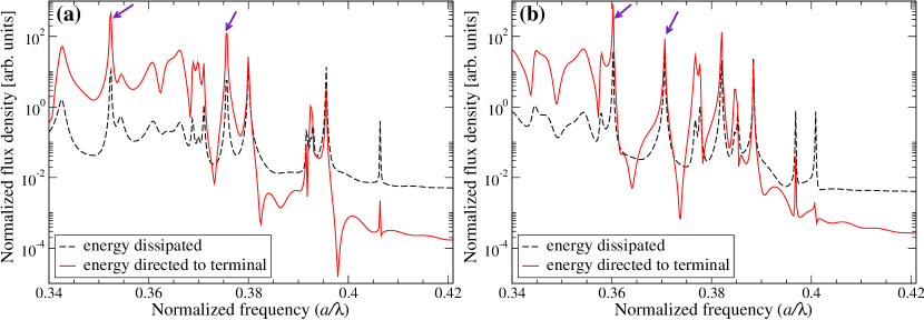
Figure 7: The normalized energy flux through the terminal (red solid line) and elsewhere (black dashed line) for a 3-row Cantor waveguide with $\Delta=0.75a$ (a) and $\Delta=a$ (b). Arrows indicate the resonant peaks under study, shown in Table 1.

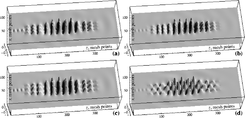
Figure 8: Normalized electric field distribution of resonant modes for the 3-row Cantor nanopillar waveguide with the distance $\Delta=0.75a$ (a,b) and $\Delta=a$ (c,d) for the two different resonant peaks (designated by arrows in Fig. 7).

In Section II we have shown that the resonant mode Q-factors of Cantor nanopillar waveguides increase by almost a factor of ten and can compete with that of a point defect resonator, when arranged in a multiple-row fashion (see, e.g., Fig. 1d). In contrast, there is no substantial increase of Q-factor for Fibonacci structures. In this section, we therefore study the radiation pattern of resonant modes in aperiodic multiple-row waveguides, resorting further to Cantor structures only.

As in the previous section, we begin the analysis by considering the spatial redistribution of the energy fluxes into the terminal and elsewhere for different frequencies in the spectrum. For the results to be comparable to those obtained above, the terminal was chosen to be identical, even though with respect to device design it might be advantageous to increase its width along with the lateral size of the multiple-row waveguide. According to our above mentioned results, the terminal was positioned so as to break the waveguide symmetry. Taking into account the width of the terminal, this amounts to the leftmost nanopillar in the central row being removed, and the terminal tip being inserted in its place. This is obviously advantageous over removing the leftmost pillar from all rows because the latter case would additionally increase radiation losses.

The results are depicted in Fig. 7. In general, the picture looks much the same as in Fig. 4c, however with an increased number of peaks and an increased Q-factor of the modes (see Table 1). Detailed analysis shows that for some peaks the ratio $\zeta$ can be as high as 20–30, providing an even better coupling between the mode and the terminal. Thus, some resonant modes in multiple-row Cantor waveguides combine a Q-factor as high as for the point defect and an excellent coupling with the external terminal. $\eta$ may be estimated to be 4–5 orders of magnitude better than in the reference point-defect structure.

For illustration, we have chosen two peaks for each value of lateral spacing $\Delta$, shown in Table 1. The results for the electric field distribution are shown in Fig. 8. Comparing those with Fig. 6, we see that the field amplitude inside the terminal is in general much greater than that of the sideways radiation losses.

V Conclusion

To summarize, we have theoretically investigated resonant modes in single- and multiple-row deterministically aperiodic nanopillar waveguides, in comparison to a point defect in a periodic reference system.

Our calculations indicate that for certain resonance frequencies the Fibonacci and Cantor nanopillar waveguides do exhibit relatively high Q-factors along with improved coupling of the radiation to an external terminal. In gereral associated Q-factors are up to the order of magnitude lower with respect to the reference defect structure, while the amount of the radiation coupled to the terminal can be up to several orders of magnitude larger in the aperiodic structures. These may be traced back to the greater spatial extension of the modes along the aperiodic waveguide and to the strong anisotropy of their radiation pattern, with large fraction of power radiated into the direction of the longitudinal waveguide axis. The coupling to the external waveguide can be further enhanced when the structure’s internal symmetry is broken by the waveguide overlapping spatially with the aperiodic structure. Even a slight symmetry breaking (removing one nanopillar from the terminal end of the structure) induces a significant coupling increase, while reducing the Q-factor by only about 10 per cent. We found by contrast that, in order to achieve a similar coupling in a periodic waveguide with point defect, one would need to place the defect as close as 3 nanopillars away from the terminal, which would, however, diminish the Q-factor by two orders of magnitude.

The Q-factor of single-row aperiodic waveguides is in general smaller by roughly an order of magnitude as compared to a point-defect resonator in a periodic structure. However, it becomes comparable to that of the reference point-defect system when multiple-row Cantor waveguides are used. Multiple-row Fibonacci waveguides do not show a significant Q-factor increase.

We conclude that, in terms of simultaneous Q-factor and terminal coupling ($\zeta$) optimization, the Cantor structure appears to be the most favourable one among the ones studied here. However, we have only studied two out of many cases of deterministically aperiodic sequences. In this context it is worth to investigate other quasiperiodic and fractal structures as well. Deterministically aperiodic structures can also be employed in the design of other types of photonic crystal waveguides, which is also a promising subject of further research. For example, by inserting 1D quasi-periodic sequence of rods or holes into a photonic crystal waveguide one can introduce new resonances into the transmission characteristic of the waveguide, while the scattering loss should be dramatically reduced due to the presence of the full 2D photonic bandgap in the surrounding 2D lattice.

- (1) J. D. Joannopoulos, R. D. Meade, and J. N. Winn, Photonic Crystals: Molding the Flow of Light (Princeton University Press, Princeton, 1995).
- (2) K. Sakoda, Optical Properties of Photonic Crystals (Princeton Springer, Berlin, 2001).
- (3) D. Englund, I. Fushman, J. Vučković, General recipe for designing photonic crystal cavities, Opt. Express 13, 5961–5975 (2005).
- (4) H. Benisty, D. Labilloy, C. Weisbuch, C. J. M. Smith, T. F. Krauss, D. Kassagne, A. Béraud, C. Jouanin, Radiation losses of waveguide-based two-dimensional protonic crystals: Positive role of the substrate, Appl. Phys. Lett. 76, 532–534 (2000).
- (5) C. Kim, W. J. Kim, A. Stapleton, J.–R. Cao, J. D. O’Brien, P. D. Dapkus, Quality factors in single-defect photonic crystal lasers with asymmetric cladding layers, J. Opt. Soc. Am. B 19, 1777–1781 (2002).
- (6) S.-H. Kwon, Y.-H. Lee, High index-contrast 2D photonic band-edge laser, IEICE Trans. Electron. E87–C, 308–315 (2004).
- (7) H. Cao, Review on latest developments in random lasers with coherent feedback, J. Phys. A: Math. Gen., 38 10497–10535 (2005).
- (8) A. L. Burin, H. Cao, G. C. Schatz, M. A. Ratner, High-quality modes in low-dimensional array of nanoparticles: application to random lasers, J. Opt. Soc. Am. B 21, 121–131 (2004).
- (9) S. Fan, J. Winn, A. Devenyi, J. C. Chen, R. D. Meade, and J. D. Joannopoulos, Guided and defect modes in periodic dielectric waveguides, J. Opt. Soc. Amer. B, 12, 1267–1272 (1995).
- (10) D. N. Chigrin, A. V. Lavrinenko, C. M. Sotomayor-Torres, Nanopillars protonic crystal waveguides, Opt. Express 12, 617–622 (2004).
- (11) D. N. Chigrin, A. V. Lavrinenko, C. M. Sotomayor-Torres, Numerical characterization of nanopillar protonic crystal waveguides and directional couplers, Optical and Quantum Electronics 37, 331–341 (2005).
- (12) M. Tokushima, H. Yamada, Y. Arakawa, 1.5-m-wavelength light guiding in waveguides in square-lattice-of-rod photonic crystal slab, Appl. Phys. Lett. 84, 4298–4300 (2004).
- (13) S. Assefa, P. T. Rakich, P. Bienstman, S. G. Johnson, G. S. Petrich, J. D. Joannopoulos, L. A. Kolodziejski, E. P. Ippen, H. I. Smith, Guiding 1.5 m light in photonic crystals based on dielectric rods, Appl. Phys. Lett. 85, 6110–6112 (2004).
- (14) E. Schonbrun, M. Tinker, W. Park and J.–B. Lee, Negative Refraction in a Si-Polymer Photonic Crystal Membrane, IEEE Photon. Technol. Lett. 17, 1196–1198 (2005).
- (15) J. C. Johnson, H. Yan, R. D. Schaller, L. H. Haber, R. J. Saykally, P. Yang, Single nanowire lasers, J. Phys. Chem. B 105, 11387–11390 (2001).
- (16) S. G. Johnson, S. Fan, A. Mekis, J. D. Joannopoulos, Multipole-cancellation mechanism for high- cavities in the absence of a complete photonic band gap, Appl. Phys. Lett. 78, 3388–3390 (2001).
- (17) M. Kohmoto, B. Sutherland, C. Tang, Critical wave function and a Cantor-set spectrum of a one-dimensional quasicrystal model, Phys. Rev. B 35, 1020–1033 (1987).
- (18) A. V. Lavrinenko, S. V. Zhukovsky, K. S. Sandomirskii, S. V. Gaponenko, Propagation of classical waves in nonperiodic media: Scaling properties of an optical Cantor filter, Phys. Rev. E 65, 036621 (2002).
- (19) C. Janot, Quasicrystals: A primer (Oxford, Clarendon Press, 1994).
- (20) S. V. Zhukovsky, A. V. Lavrinenko, S. V. Gaponenko, Spectral scalability as a result of geometrical self-similarity in fractal multilayers, Europhys. Lett. 66, 455–461 (2004).
- (21) A. V. Lavrinenko, P. I. Borel, L. H. Fradsen, M. Thorhauge, A. Harpøth, M. Kristensen, T. Niemi, H. Chong, Comprehensive FDTD modelling of photonic crystal waveguide components, Opt. Express 12, 234–248 (2004)
- (22) J. P. Berenger, A perfectly matched layer for the absorption of electromagnetic waves, J. Comp. Phy. 114, 185–200(1994)
- (23) V. V. Zosimov, L. M. Lyamshev, Fractals in wave processes, Physics – Uspekhi 38, 347–384 (2005).