Topologization of electron liquids with Chern-Simons theory and quantum computation

1. Introduction

In 1987 a Geometry and Topology year was organized by Prof. Chern in Nankai and I participated as an undergraduate from the University of Science and Technology of China. There I learned about M. Freedman’s work on 4-dimensional manifolds. Then I went to the University of California at San Diego to study with M. Freedman in 1989, and later became his most frequent collaborator. It is a great pleasure to contribute an article to the memory of Prof. Chern based partially on some joint works with M. Freedman and others. Most of the materials are known to experts except some results about the classification of topological quantum field theories (TQFTs) in the end. This paper is written during a short time, so inaccuracies are unavoidable. Comments and questions are welcome.

There are no better places for me to start than the Chern-Simon theory. In the hands of Witten, the Chern-Simons functional is used to define TQFTs which explain the evaluations of the Jones polynomial of links at certain roots of unity. It takes great imagination to relate the Chern-Simons theory to electrons in magnetic fields, and quantum computing. Nevertheless, such a nexus does exist and I will outline this picture. No attempt has been made regarding references and completeness.

2. Chern-Simons theory and TQFTs

Fix a simply connected Lie group $G$. Given a closed oriented 3-manifold $M$ and a connection $A$ on a principle $G$-bundle $P$ over $M$, the Chern-Simons 3-form $\textrm{tr}(A\wedge dA+\frac{2}{3}A^{3})$ is discovered when Profs. Chern and Simons tried to derive a purely combinatorial formula for the first Pontrjagin number of a 4-manifold. Let $CS(A)=\frac{1}{8\pi^{2}}\int_{M}\textrm{tr}(A\wedge dA+\frac{2}{3}A^{3})$ be the Chern-Simons functional. To get a TQFT, we need to define a complex number for each closed oriented 3-manifold $M$ which is a topological invariant, and a vector space $V(\Sigma)$ for each closed oriented 2-dimensional surface $\Sigma$. For a level $k\geq h^{\vee}+1$, where $h^{\vee}$ is the dual Coxeter number of $G$, the 3-manifold invariant of $M$ is the path integral $Z_{k}(M^{3})=\int_{A}e^{2\pi i\cdot k\cdot CS(A)}DA$, where the integral is over all gauge-classes of connection on $P$ and the measure $DA$ has yet to be defined rigorously. A closely related 3-manifold invariant is discovered rigorously by N. Reshetikhin and V. Turaev based on quantum groups. To define a vector space for a closed oriented surface $\Sigma$, let $X$ be an oriented 3-manifold whose boundary is $\Sigma$. Consider a principle $G$-bundle $P$ over $X$, fix a connection $a$ on the restriction of $P$ to $\Sigma$, let $Z_{k,a}=\int_{(A,a)}e^{2\pi i\cdot k\cdot CS(A)}DA$, where the integral is over all gauge-classes of connections of $A$ on $P$ over $X$ whose restriction to $\Sigma$ is $a$. This defines a functional on all connections $\{a\}$ on the principle $G$-bundle $P$ over $\Sigma$. By forming formal finite sums, we obtain an infinite dimensional vector space $S(\Sigma)$. In particular, a 3-manifold $X$ such that $\partial X=\Sigma$ defines a vector in $S(\Sigma)$. Path integral on disks introduces relations onto the functionals, we get a finitely dimensional quotient of $S(\Sigma)$, which is the desired vector space $V(\Sigma)$. Again such finitely dimensional vector spaces are constructed mathematically by N. Reshetikhin and V. Turaev. The 3-manifold invariant of closed oriented 3-manifolds and the vectors spaces associated to the closed oriented surfaces form part of the Witten-Reshetikhin-Turaev-Chern-Simons TQFT based on $G$ at level=$k$. Strictly speaking the 3-manifold invariant is defined only for framed 3-manifolds. This subtlety will be ignored in the following.

Given a TQFT and a closed oriented surface $\Sigma$ with two connected components $\overline{\Sigma_{1}},\Sigma_{2}$, where $\overline{\Sigma_{1}}$ is $\Sigma_{1}$ with the opposite orientation, a 3-manifold $X$ with boundary $\partial X=\Sigma$ gives rise to a linear map from $V(\Sigma_{1})$ to $V(\Sigma_{2})$. Then the mapping cylinder construction for self-diffeomorphisms of surfaces leads to a projective representation of the mapping class groups of surfaces. This is the TQFT as axiomatized by M. Atiyah. Later G. Moore and N. Seiberg, K. Walker and others extended TQFTs to surfaces with boundaries. The new ingredient is the introduction of labels for the boundaries of surfaces. For the Chern-Simons TQFTs, the labels are the irreducible representations of the quantum deformation groups of $G$ at level=$k$ or the positive energy representations of the loop groups of $G$ at level=$k$. For more details and references, see [T].

3. Electrons in a flatland

Eighteen years before the discovery of electron, a graduate student E. Hall was studying Electricity and Magnetism using a book of Maxwell. He was puzzled by a paragraph in Maxwell’s book and performed an experiment to test the statement. He disproved the statement by discovering the so-called Hall effect. In 1980, K. von Klitzing discovered the integer quantum Hall effect (IQHE) which won him the 1985 Nobel Prize. Two years later, H. Stormer, D. Tsui and A. Gossard discovered the fractional quantum Hall effect (FQHE) which led to the 1998 Nobel Prize for H. Stormer, D. Tsui and R. Laughlin. They were all studying electrons in a 2-dimensional plane immersed in a perpendicular magnetic field. Laughlin’s prediction of the fractional charge of quasi-particles in FQHE electron liquids is confirmed by experiments. Such quasi-particles are anyons, a term introduced by F. Wilczek. Braid statistics of anyons are deduced, and experiments to confirm braid statistics are being pursued.

The quantum mechanical problem of an electron in a magnetic field was solved by L. Landau. But there are about $10^{11}$ electrons per $cm^{2}$ for FQHE liquids, which render the solution of the realistic Hamiltonian for such electron systems impossible, even numerically. The approach in condensed matter physics is to write down an effective theory which describes the universal properties of the electron systems. The electrons are strongly interacting with each other to form an incompressible electron liquid when the FQHE could be observed. Landau’s solution for a single electron in a magnetic field shows that quantum mechanically an electron behaves like a harmonic oscillator. Therefore its energy is quantized to Landau levels. For a finite size sample of a 2-dimensional electron system in a magnetic field, the number of electrons in the sample divided by the number of flux quanta in the perpendicular magnetic field is called the Landau filling fraction $\nu$. The state of an electron system depends strongly on the Landau filling fraction. For $\nu<1/5$, the electron system is a Wigner crystal: the electrons are pinned at the vertices of a triangular lattice. For $\nu$ is an integer, the electron system is an IQHE liquid, where the interaction among electrons can be neglected. When $\nu$ are certain fractions such as $1/3,1/5,...$, the electrons are in a FQHE state. Both IQHE and FQHE are characterized by the quantization of the Hall resistance $R_{xy}=\nu^{-1}\frac{h}{e^{2}}$, where $e$ is the electron charge and $h$ the Planck constant, and the exponentially vanishing of the longitudinal resistance $R_{xx}$. There are about 50 such fractions and the quantization of $R_{xy}$ is reproducible up to $10^{-10}$. How could an electron system with so many uncontrolled factors such as the disorders, sample shapes and strength of the magnetic fields, quantize so precisely? The IQHE has a satisfactory explanation both physically and mathematically. The mathematical explanation is based on non-commutative Chern classes. For the FQHE at filling fractions with odd denominators, the composite fermion theory based on U(1)-Chern-Simons theory is a great success: electrons combined with vortices to form composite fermions and then composite fermions, as new particles, to form their own integer quantum Hall liquids. The exceptional case is the observed FQHE $\nu=5/2$. There are still very interesting questions about this FQH state. For more details and references see [G].

4. Topologization of electron liquids

The discovery of the fractional quantum Hall effect has cast some doubts on Landau theory for states of matter. A new concept, topological order, is proposed by Xiao-gang Wen of MIT. It is believed that the electron liquid in a FQHE state is in a topological state with a Chern-Simons TQFT as an effective theory. In general topological states of matter have TQFTs as effective theories. The $\nu=5/2$ FQH electron liquid is still a puzzle. The leading theory is based on the Pfaffian states proposed by G. Moore and N. Read in 1991 [MR]. In this theory, the quarsi-particles are non-abelian anyons (a.k.a. plectons) and the non-abelian statistics is described by the Chern-Simons-SU(2) TQFT at level=2.

To describe the new states of matter such as the FQH electron liquids, we need new concepts and methods. Consider the following Gedanken experiment: suppose an electron liquid is confined to a closed oriented surface $\Sigma$, for example a torus. The lowest energy states of the system form a Hilbert space $V(\Sigma)$, called the ground states manifold. In an ordinary quantum system, the ground state will be unique, so $V(\Sigma)$ is 1-dimensional. But for topological states of matter, the ground states manifold is often degenerate (more than 1-dimensional), i.e. there are several orthogonal ground states with exponentially small energy differences. This ground states degeneracy is a new quantum number. Hence a topological quantum system assigns each closed oriented surface $\Sigma$ a Hilbert space $V(\Sigma)$, which is exactly the rule for a TQFT. FQH electron liquid always has an energy gap in the thermodynamic limit which is equivalent to the incompressibility of the electron liquid. Therefore the ground states manifold is stable if controlled below the gap. Since the ground states manifold has the same energy, the Hamiltonian of the system restricted to the ground states manifold is 0, hence there will be no continuous evolutions. This agrees with the direct Lengendre transform form the Chern-Simons Lagrangians to Hamiltoninans. Since the Chern-Simons 3-form has only first derivatives, the corresponding Hamiltonian is identically 0. In summary, ground states degeneracy, energy gap and the vanishing of the Hamiltonian are all salient features of topological quantum systems.

Although the Hamiltonian for a topological system is identically 0, there are still discrete dynamics induced by topological changes. In this case the Schrodinger equation is analogous to the situation for a function $f(x)$ such that $f^{\prime}(x)=0$, but there are interesting solutions if the domain of $f(x)$ is not connected as then $f(x)$ can have different constants on the connected components. This is exactly why braid group representations arise as dynamics of topological quantum systems.

5. Anyons and braid group representations

Elementary excitations of FQH liquids are quasi-particles. In the following we will not distinguish quasi-particles from particles. Actually it is not inconceivable that particles are just quasi-particles from some complicated vacuum systems. Particle types serve as the labels for TQFTs. Suppose a topological quantum system confined on a surface $\Sigma$ has elementary excitations localized at certain points $p_{1},p_{2},\cdots$ on $\Sigma$, the ground states of the system outside some small neighborhoods of $p_{i}$ form a Hilbert space. This Hilbert space is associated to the surface with the small neighborhoods of $p_{i}$ deleted and each resulting boundary circle is labelled by the corresponding particle type. Although there are no continuous evolutions, there are discrete evolutions of the ground states induced by topological changes such as the mapping class groups of $\Sigma$ which preserve the boundaries and their labels. An interesting case is the mapping class groups of the disk with $n$ punctures—the famous braid groups on $n$-strands, $B_{n}$.

Another way to describe the braid groups $B_{n}$ is as follows: given a collection of $n$ particles in the plane ${\mathbb{R}}^{2}$, and let $I=[t_{0},t_{1}]$ be a time interval. Then the trajectories of the particles will be $n$ disjoint curves in ${\mathbb{R}}^{2}\times I$ if at any moment the $n$ particles are kept apart from each other. If the $n$ particles at time $t_{1}$ return to their initial positions at time $t_{0}$ as a set, then their trajectories form an $n$-braid $\sigma$. Braids can be stacked on top of each other to form the braid groups $B_{n}$. Suppose the particles can be braided adiabatically so that the quantum system would be always in the ground states, then we have a unitary transformation from the ground states at time $t_{0}$ to the ground states at time $t_{1}$. Let $V(\Sigma)$ be the Hilbert space for the ground states manifold, then a braid induces a unitary transformation on $V(\Sigma)$. Actually those unitary transformations give rise to a projective representation of the braid groups. If the $n$ particles are of the same type, the resulting representations of the braid groups will be called the braid statistics. Note that there is a group homomorphism from the braid group $B_{n}$ to the permutation groups $S_{n}$ by remembering only the initial and final positions of the $n$ particles.

The plane ${\mathbb{R}}^{2}$ above can be replaced by any space $X$ and statistics can be defined for particles in $X$ similarly. The braid groups are replaced by the fundamental groups $B_{n}(X)$ of the configuration spaces $C_{n}(X)$. If $X={\mathbb{R}}^{m}$ for some $m>2$, it is well known that $B_{n}(X)$ is $S_{n}$. Therefore, all particle statistics will be given by representations of the permutation groups. There are two irreducible 1-dimensional representations of $S_{n}$, which correspond to bosons and fermions. If the statistics does not factorize through the permutation groups $S_{n}$, the particles are called anyons. If the images are in $U(1)$, the anyon will be called abelian, and otherwise non-abelian. The quasi-particles in the FQH liquid at $\nu=1/3$ are abelian anyons. To be directly useful for topological quantum computing, we need non-abelian anyons. Do non-abelian anyons exist?

Mathematically are there unitary representations of the braid groups? There are many representations of the braid groups, but unitary ones are not easy to find. The most famous representations of the braid groups are probably the Burau representation discovered in 1936, which can be used to define the Alexander polynomial of links, and the Jones representation discovered in 1981, which led to the Jones polynomial of links. It is only in 1984 that the Burau representation was observed to be unitary by C. Squier, and the Jones representation is unitary as it was discovered in a unitary world [J1]. So potentially there could be non-abelian anyon statistics. An interesting question is: given a family of unitary representations of the braid groups $\rho_{n}:B_{n}\rightarrow U(k_{n})$, when this family of representations can be used to simulate the standard quantum circuit model efficiently and fault tolerantly? A sufficient condition is that they come from a certain TQFT, but is it necessary?

Are there non-abelian anyons in Nature? This is an important unknown question at the writing. Experiments are underway to confirm the prediction of the existence in certain FQH liquids [DFN]. Specifically the FQH liquid at $\nu=5/2$ is believed to have non-abelian anyons whose statistics is described by the Jones representation at the 4-th root of unity. More generally N. Read and E. Rezayi conjectured that the Jones representation of the braid groups at r-th root of unity describes the non-abelian statistics for FQH liquids at filling fractions $\nu=2+\frac{k}{k+2}$, where $k=r-2$ is the level [RR]. For more details and references on anyons see [Wi].

As an anecdote, a few years ago I wrote an article with others about quantum computing using non-abelian anyons and submitted it to the journal Nature. The paper was rejected within almost a week with a statement that the editors did not believe in the existence of non-abelian anyons. Fortunately the final answer has to come from Mother Nature, rather than the journal Nature.

6. Topological quantum computing

In 1980s Yu. Manin and R. Feynman articulated the possibility of computing machines based on quantum physics to compute much faster than classical computers. Shor’s factoring algorithm in 1994 has dramatically changed the field and stirred great interests in building quantum computers. There are no theoretical obstacles for building quantum computers as the accuracy threshold theorem has shown. But decoherence and errors in implementing unitary gates have kept most experiments to just a few qubits. In 1997 M. Freedman proposed the possibility of TQFT computing [F]. Independently A. Kitaev proposed the idea of fault tolerant quantum computing using anyons [K]. The two ideas are essentially equivalent as we have alluded before. Leaving aside the issue of discovering non-abelian anyons, we may ask how to compute using non-abelian anyons? For more details and references see [NC].

6.1. Jones representation of the braid groups

Jones representation of the braid groups is the same as the Witten-Reshetikhin-Turaev-SU(2) TQFT representation of the braid groups. Closely related theories can be defined via the Kaffuman bracket. For an even level $k$, the two theories are essentially the same, but for odd levels the two theories are distinguished by the Frobenius-Schur indicators. However the resulting braid group representations are the same. Therefore we will describe the braid group representations using the Kauffman bracket. The Kauffman bracket is an algebra homomorphism from the group algebras of the braid groups $\mathbb{C}[B_{n}]$ to the generic Temperley-Lieb algebras. For applications to quantum computing we need unitary theories. So we specialize the Kauffman variable $A$ to certain roots of unity. The resulting algebras are reducible. Semi-simple quotients can be obtained by imposing the Jones-Wenzl idempotents. The semi-simple quotient algebras will be called the Jones algebras, which are direct sum of matrix algebras. Fix $r$ and an $A$ satisfying $A^{4}=e^{\pm 2\pi i/r}$, the Jones representation for a braid $\sigma$ is the Kauffman bracket image in the Jones algebra. To describe the Jones representation, we need to find the decomposition of the Jones algebras into their simple matrix components (irreducible sectors). The set of particle types for the Chern-Simons-SU(2) TQFT at level=$k$ is $L=\{0,1,\cdots,k\}$. The fusion rules are given by $a\otimes b=\oplus c$, where $a,b,c$ satisfy

1). the sum $a+b+c$ is even,

2). $a+b\geq c,b+c\geq a,c+a\geq b$,

3). $a+b+c\leq 2k$.

A triple $(a,b,c),a,b,c\in L$ satisfying the above three conditions will be called admissible.

The Jones algebra at level=$k$ for n-strands decomposes into irreducible sectors labeled by an integer $m$ such that $m\in L,m=n\;mod\;2$. Fix $m$, the irreducible sector has a defining representation $V^{m}_{1^{n}}$ with a basis consisting of admissible labelings of the following tree (Fig. 1):

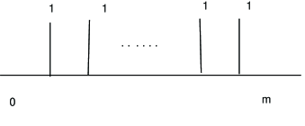
Figure 1. Basis

There are $n$ vertical edges labeled by 1, and the 0-th horizontal edge (leftmost) is always labeled by 0, and the n-th edge (rightmost) is always labeled by $m$. The internal $(n-1)$ edges are labeled by $a,b,c,\cdots$ such that any three labels incident to a trivalent vertex form an admissible triple. A basis with internal labelings $a,b,c,\cdots$ will be denoted by $e^{m}_{a,b,c,\cdots}$. The Kauffman bracket is $\sigma_{i}=A\cdot\textrm{id}+A^{-1}\cdot U_{i}$, so it suffices to describe the matrix for $U_{i}$ with basis $e^{m}_{a,b,c,\cdots}$ in $V^{m}_{1^{n}}$. The matrix for $U_{i}$ consists of $1\times 1$ and $2\times 2$ blocks. Fix $m$ and a basis element $e^{m}_{a,b,c,\cdots}$, suppose that the $i,i+1,i+2$ internal edges are labeled by $f,g,h$. If $f\neq h$, then $U_{i}$ maps this basis to 0. If $f=h$, then by the fusions rules $g=f\pm 1$ (the special case is $f=0$, then $g=1$ only), then $U_{i}$ maps $e^{m}_{\cdots,f,f\pm 1,f,\cdots}$ back to themselves by the following $2\times 2$ matrix:

$$\left(\begin{array}[]{cc}\frac{\Delta_{f+1}}{\Delta_{f}}&x\\ y&\frac{\Delta_{f-1}}{\Delta_{f}}\end{array}\right),$$

where $\Delta_{k}$ is the Chebyshev polynomial defined by $\Delta_{0}=1,\Delta_{1}=d,\Delta_{k+1}=d\Delta_{k}+\Delta_{k-1},d=-A^{2}-A^{-2}$, and $x,y$ satisfy $xy=\frac{\Delta_{f+1}\Delta_{f-1}}{\Delta_{f}^{2}}$.

From those formulas, there is a choice of $x,y$ up to a scalar, and in order to get a unitary representation, we need to choose $A$ so that the $2\times 2$ blocks are real symmetric matrices. This forces $A$ to satisfy $q=A^{4}=e^{\pm 2\pi i/r}$. It also follows that the eigenvalues of $\sigma_{i}$ are $-1,q$ up to scalars.

6.2. Anyonic quantum computers

We will use the level=2 theory to illustrate the construction of topological quantum computers. There are three particle types $\{0,1,2\}$. The label 0 denotes the null-particle type, which is the vacuum state. Particles of type 1 are believed to be non-abelian anyons. Consider the unitary Jones representation of $B_{4}$, the irreducible sector with $m=0$ has a basis $\{e^{0}_{1,b,1}\}$, where $b=0$ or $2$. Hence this can be used to encode a qubit. For $B_{6}$, a basis consists of $e^{0}_{1,b_{1},1,b_{2},1}$, where $b_{i},i=1,2$ is $0$ or $2$. Hence this can be used to encode 2-qubits. In general n-qubits can be encoded by the $m=0$ irreducible sector of the Jones representation $\rho^{0}_{2n+2}$ of $B_{2n+2}$. The unitary matrices of the Jones representations $\rho_{4}^{0}(B_{4}),\rho_{4}^{0}(B_{6})$ will be quantum gates. To simulate a quantum circuit on n-qubits $U_{L}:{(\mathbb{C}^{2})}^{\otimes n}\rightarrow{(\mathbb{C}^{2})}^{\otimes n}$, we need a braid $\sigma\in B_{2n+2}$ such that the following diagram commutes:

This is not always possible because the images of the Jones representation of the braid groups at $r=4$ are finite groups. It follows that the topological model at $r=4$ is not universal. To get a universal computer, we consider other levels of the Chern-Simons-SU(2) TQFT. The resulting model for $r=4$ is slightly different from the above one. To simulate n-qubits, we consider the braid group $B_{4n}$. The 4n edges besides the leftmost in Fig. 1 can be divided into n groups of 4. Consider the basis elements such every 4k-th edge is labelled by 0, and every (4k+2)-th edge can be labeled either by 0 or 2. Those $2^{n}$ basis elements will be used to encode n-qubits. The representations of the braid groups $B_{4n}$ will be used to simulate any quantum circuits on n-qubits. This is possible for any level other than 1,2 and 4 [FLW1][FLW2].

6.3. Measurement in topological models

A pictorial illustration of a topological quantum computer is as follows (Fig. 2):

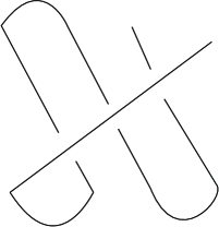
Figure 2. Topological model

We start the computation with the ground states of a topological system, then create particle pairs from the ground states to encode the initial state which is denoted by $|cup>$(two bottom cup). A braid $b$ is adiabatically performed to induce the desired unitary matrix $\rho(b)$. In the end, we annihilate the two leftmost quasi-particles (the top cap) and record the particle types of the fusion. Then we repeat the process polynomially many times to get an approximation of the probability of observing any particle type. Actually we need only to distinguish the trivial versus all other non-trivial particle types. For level=3 or $r=5$, the probability to observe the trivial particle type 0 is $<cap|\rho^{+}(b)\prod_{0}\rho(b)|cup>$, which is related to the Jones polynomial of the following circuit link (Fig. 3) by the formula:

$$p=\textrm{prob}(0)=\frac{1}{1+[2]^{2}}(1+\frac{(-1)^{c}\cdot V_{L}(e^{2\pi i/5})}{[2]^{c-2}}),$$

Figure 3. Circuit link

where in the formula $c=c(L)$ is the number of components of the link L, $[2]=-A^{2}-A^{-2}$ is quantum 2 ar $r=5$. Our normalization for the Jones polynomial is that for the unlink with c components, the Jones polynomial is $(-[2])^{c}$.

To derive this formula, we assume the writhe of L is 0. Other cases are similar. In the Kauffman bracket formulation, the projector to null particle type $\prod_{0}$ is the same as the element $\frac{U_{1}}{-[2]}$ of the Jones algebras. It follows that $p$ is just the Kauffman bracket of the tangle $b\cdot U_{1}\cdot b^{-1}$ divided by $-[2]$. Now consider the Kaffman bracket $<L>$ of $L$, resolving the 4 crossings of $L$ on the component $\gamma$ using the Kauffman bracket results a sum of 16 terms. Simplifying, we get

$$<L>=(-[2])^{c}([2]^{2}-3)+(4-[2]^{2})(-[2])^{c}\cdot p.$$

Since the writhe is assumed to be 0, the Kauffman bracket is the same as the Jones polynomial of $L$. Solving for $p$, we obtain

$$p=\frac{3-[2]^{2}}{4-[2]^{2}}(1+\frac{(-1)^{c}\cdot V_{L}(e^{2\pi i/5})}{[2]^{c}\cdot(3-[2]^{2})}.$$

Direct calculation using the identity $[2]^{2}=1+[2]$ gives the desired formula. This formula shows that if non-abelian anyons exist to realize the Jones representation of the braid groups, then quantum computers will approximate the Jones polynomial of certain links. So the Jones polynomial of links are amplitudes for certain quantum processes [FKLW]. This inspired a definition of a new approximation scheme: the additive approximation which might lead to a new characterization of the computational class BQP [BFLW].

6.4. Universality of topological models

In order to simulate all quantum circuits, it suffices to have the closed images of the braid groups representations containing the special unitary groups for each representation space. In 1981 when Jones discovered his revolutionary unitary representation of the braid groups, he proved that the images of the irreducible sectors of his unitary representation are finite if $r=1,2,3,4,6$ for all $n$ and $r=10$ for $n=3$. For all other cases the closed images are infinite modulo center. He asked what are the closed images? In the joint work with M. Freedman, and M. Larsen [FLW2], we proved that they are as large as they can be: always contain the special unitary groups. As a corollary, we have proved the universality of the anyonic quantum computers for $r\neq 1,2,3,4,6$.

The proof is interesting in its own right as we formulated a two-eigenvalue problem and found its solution [FLW2]. The question of understanding TQFT representations of the mapping class groups are widely open. Partial results are obtained in [LW].

6.5. Simulation of TQFTs

In another joint work with M. Freedman, and A. Kitaev [FKW], we proved that any unitary TQFT can be efficiently simulated by a quantum computer. Combined with the universality for certain TQFTs, we established the equivalence of TQFT computing with quantum computing. As corollaries of the simulation theorem, we obtained quantum algorithms for approximating quantum invariants such as the Jones polynomial. Jones polynomial is a specialization of the Tutte polynomial of graphs. It is interesting to ask if there are other partition functions that can be approximated by quantum computers efficiently [Wel].

6.6. Fault tolerance of topological models

Anyonic quantum computers are inherently fault tolerant [K]. This is essentially a consequence of the disk axiom of TQFTs if the TQFTs can be localized to lattices on surfaces. Localization of TQFTs can also be used to establish an energy gap rigorously.

7. Classification of topological states of matter

Topological orders of FQH electron liquids are modelled by TQFTs. It is an interesting and difficult problem to classify all TQFTs, hence topological orders. In 2003 I made a conjecture that if the number of particle types is fixed, then there are only finitely many TQFTs. The best approach is based on the concept of modular tensor category (MTC) [T][BK]. A modular tensor category encodes the algebraic data inside a TQFT, and describes the consistency of an anyonic system. Modular tensor category might be a very useful concept to study topological quantum systems. In 2003 I gave a lecture at the American Institute of Mathematics to an audience of mostly condensed matter physicists. It was recognized by one of the participants, Prof. Xiao-gang Wen of MIT, that indeed tensor category is useful for physicists as his recent works have shown.

Recently S. Belinschi, R. Stong, E. Rowell and myself have achieved the classification of all MTCs up to 4 labels. The result has not been written up yet, but the list is surprisingly short. Each fusion rule is realized by either a Chern-Simons TQFT and its quantum double. For example, the fusion rules of self-dual, singly generated modular tensor categories up to rank=4 are realized by: $SU(2)$ level=1, $SO(3)$ level=3, $SU(2)$ level=2, $SO(3)$ level 5, $SU(2)$ level=3.

8. Open questions

There are many open problems in the subject and directions to pursue for mathematicians, physicists and computer scientists. We just mention a few here. The most important for the program is whether or not there are non-abelian anyons in Nature. Another question is to understand the boundary (1+1) quantum field theories of topological quantum systems. Most of the boundary QFTs are conformal field theories. What is the relation of the boundary QFT with the bulk TQFT? How do we classify them?

Quantum mechanics has been incorporated into almost every physical theory in the last century. Mathematics is experiencing the same now. Wavefunctions may well replace the digital numbers as the new notation to describe our world. The nexus among quantum topology, quantum physics and quantum computation will lead to a better understanding of our universe, and Prof. Chern would be happy to see how important a role that his Chern-Simons theory is playing in this new endeavor.

References

- [BK] B. Bakalov and A. Kirillov Jr., Lectures on tensor categories and modular functions, Amer. Math. Soc., Providence, RI, 2001.
- [BFLW] M. Bordewich, M. Freedman, L. Lov sz, and D. Welsh, Approximate Counting and Quantum Computation, Combinatorics, Probability and Computing archive Volume 14 , Issue 5-6 (November 2005).
- [DFN] S. Das Sarma, M. Freedman, and C. Nayak, Topologically-Protected Qubits from a Possible Non-Abelian Fractional Quantum Hall State, Phys. Rev. Lett. 94, 166802 (2005).
- [F] M. Freedman, P/NP, and the quantum field computer. Proc. Natl. Acad. Sci. USA 95 (1998), no. 1, 98 101.
- [FKW] M. H. Freedman, A. Kitaev, and Z. Wang, Simulation of topological field theories by quantum computers, Comm. Math. Phys. 227 (2002), no.3, 587—603.
- [FKLW] M. H. Freedman, A. Kitaev, M. J. Larsen and Z. Wang, Topological quantum computation, Mathematical challenges of the 21st century (Los Angeles, CA, 2000), Bull. Amer. Math. Soc. (N.S.) 40 (2003), no. 1, 31–38.
- [FLW1] M. H. Freedman, M. J. Larsen, and Z. Wang, A modular functor which is universal for quantum computation, Comm. Math. Phys. 227 (2002),no.3,605—622.
- [FLW2] M. H. Freedman, M. J. Larsen, and Z. Wang, The two-eigenvalue problem and density of Jones representation of braid groups, Comm. Math. Phys. 228 (2002), 177-199, arXiv: math.GT/0103200.
- [G] S. Girvin, The quantum Hall effect: novel excitation and broken symmetries, Topological aspects of low dimensional systems (Les Houches - Ecole d’Ete de Physique Theorique) (Hardcover) by A. Comtet (Editor), cond-mat/9907002.
- [J1] V. F. R. Jones, Braid groups, Hecke algebras and type factors, Geometric methods in operator algebras (Kyoto, 1983), 242–273, Pitman Res. Notes Math. Ser., 123, Longman Sci. Tech., Harlow, 1986.
- [K] A. Kitaev, Fault-tolerant quantum computation by anyons, Annals Phys. 303 (2003) 2-30 ,quant-ph/9707021
- [LW] M. J. Larsen and Z. Wang, Density of the SO(3) TQFT representation of mapping class groups, Comm. Math. Phys., Volume 260(2005), Number 3, 641 - 658.
- [MR] G. Moore and N. Read, Nonaelions in the fractional quantum Hall effect, Nuc. Physc. B360(1991), 362-396.
- [NC] M. Nielsen and I. Chuang, Quantum Computation and quantum information, Cambridge University Press, 2000.
- [RR] N. Read and E. Rezayi, Beyond paired quantum Hall states: parafermions and incompressible states in first excited Landau level, Phys. Rev. B59, 8804(1999), cond-mat/9809384.
- [T] V. G. Turaev, Quantum Invariants of Knots and 3-Manifolds, de Gruyter Studies in Mathematics, 18. Walter de Gruyter Co., Berlin, 1994.
- [Wel] D. Welsh, Complexity: Knots, Colourings and Counting, LMS Lecture Notes Series 186.
- [Wi] F. Wilczek, Braid statistics and anyon superconductivity, World Scientific Pub Co Inc (December, 1990).