Critical behavior at the interface between two systems belonging to different universality classes

Abstract

We consider the critical behavior at an interface which separates two semi-infinite subsystems belonging to different universality classes, thus having different set of critical exponents, but having a common transition temperature. We solve this problem analytically in the frame of $\phi^{k}$ mean-field theory, which is then generalized using phenomenological scaling considerations. A large variety of interface critical behavior is obtained which is checked numerically on the example of two-dimensional $q$-state Potts models with $2\leq q\leq 4$. Weak interface couplings are generally irrelevant, resulting in the same critical behavior at the interface as for a free surface. With strong interface couplings, the interface remains ordered at the bulk transition temperature. More interesting is the intermediate situation, the special interface transition, when the critical behavior at the interface involves new critical exponents, which however can be expressed in terms of the bulk and surface exponents of the two subsystems. We discuss also the smooth or discontinuous nature of the order parameter profile.

I Introduction

Systems which undergo a second-order phase transition display singularities in different physical observables which have been the subject of intensive research, both experimentally and theoretically.dgl At the critical temperature, $T_{c}$, due to the existence of a diverging correlation length $\xi\sim|T-T_{c}|^{-\nu}$, microscopic inhomogeneities and single defects of finite size do not modify the critical singularities which are observed in the perfect systems.burkhardt81_rev However, inhomogeneities of infinite extent, such as the surface of the sample,binder83 ; diehl86 ; pleimling04 internal defect planes,burkhardt81 etc., may modify the local critical properties near the inhomogeneity, within a region with a characteristic size given by the correlation length. For example, the magnetization, $m$, which vanishes in the bulk as $m\sim(T_{c}-T)^{\beta}$ behaves as $m_{1}\sim(T_{c}-T)^{\beta_{1}}$ at a free surfacebinder83 ; diehl86 ; pleimling04 and the two critical exponents, $\beta$ and $\beta_{1}$, are generally different.

Inhomogeneities having a more general form, such as localizedbariev79 and extended defects,hilhorst81 corners,corner wedges and edges, parabolic shapes,peschel91 etc., often have exotic local critical behavior; for a review, see Ref. ipt93, . The local critical behavior can be nonuniversal, so that the local exponents vary continuously with some parameters, such as the opening angle of the corner,corner the amplitude of a localized,bariev79 or extended defect.hilhorst81 The inhomogeneity can also reduce the local order to such an extent that the local magnetization vanishes with an essential singularity, as observed at the tip of a parabolic-shaped system.peschel91 On the contrary, for enhanced local couplings, a surface or an interface may remain ordered at or above the bulk critical temperature,binder83 ; diehl86 ; pleimling04 which in a two-dimensional (2D) system leads to a discontinuous local transition.it93

In the problems we mentioned so far the inhomogeneities are embedded into a critical system the bulk properties of which govern, among others, the divergence of the correlation length and the behavior of the order-parameter profile. There is, however, another class of problems, in which two (or more) systems meet at an interface, each having different type of bulk (and surface) critical properties. In this respect we can mention grain boundaries between two different materials or the interface between two immiscible liquids, etc.

If the critical temperatures of the two subsystems are largely different, the nature of the transitions at the interface is expected to be the same as for a surface.berche91 At the lower critical temperature, due to the presence of the nearby ordered subsystem, the interface transition has the same properties as the extraordinary surface transition.binder83 ; diehl86 ; pleimling04 At the upper critical temperature, the second subsystem being disordered, the interface transition is actually an ordinary surface transition.binder83 ; diehl86 ; pleimling04 If the dimension of the system is larger than 2 and if the interface couplings are strong enough, one expects an interface transition in the presence of the two disordered subsystems whose properties should depend on the universality classes of these two subsystems.

Even in 2D, the local critical behavior at the interface can be more complex if the critical temperatures of the subsystems are the same or if their difference is much smaller than the deviation from their mean value. In this case an interplay or competition between the two different bulk and surface critical behaviors can result in a completely new type of interface critical phenomena. In this paper we study this problem, assuming that the critical temperatures of the two subsystems are identical.

The structure of the paper is the following. The mean-field solution of the problem including $\varphi^{3}$, $\varphi^{4}$ and $\varphi^{6}$ theories and the interface between them is presented in Sec. II. The mean-field results are generalized in Sec. III using phenomenological scaling considerations. In Sec. IV these results are confronted with Monte Carlo simulations in 2D for interfaces between subsystems belonging to the universality classes of the Ising model, the three- and four-state Potts models, as well as the Baxter-Wu (BW) model. Our results are discussed in Sec. V and some details about the analytical mean-field calculations are given in the Appendixes A and B.

II Mean-field theory

II.1 Properties of the $\bm{\varphi^{k}}$ model

II.1.1 Free energy

We consider a system with volume $V$ limited by a surface $S$ in the Landau mean-field approximation. The total free energy is the sum of bulk and surface contributions which are functionals of the scalar order parameter $\varphi(\bm{r})$ so that:binder83 ; diehl86 ; pleimling04

$$F[\varphi]=\int_{(V)}f_{b}\,[\varphi]\,dV+\int_{(S)}f_{s}\,[\varphi]\,dS\,.$$ (1)

Near a second-order transition, the order parameter is small and the bulk free energy density $f_{b}[\varphi]$ is written as an expansion in the order parameter and its gradient, limited to the following terms:

$$f_{b}\,[\varphi]=f_{b}\,[0]+\frac{C}{2}(\bm{\nabla}\varphi)^{2}+\frac{A}{2}\varphi^{2}+\frac{B}{k}\varphi^{k}-h\varphi\,.$$ (2)

The second term, with $C>0$, gives a positive contribution associated with the spatial variation of the order parameter. $A=-at$ ($a>0$, $t=T_{c}-T$) is negative when $T<T_{c}$ and measures the deviation from the critical point. The next term with $B>0$ ensures the stability of the system in the ordered phase. In the last term, $h$ is the bulk external field. When $k$ is odd, the order parameter is supposed to take only non-negative values; otherwise the system would be unstable.

In the same way the surface free energy density is written as

$$f_{s}\,[\varphi]=f_{s}\,[0]+\frac{C_{s}}{2}\frac{\varphi^{2}}{\Lambda}\,,$$ (3)

where $\varphi$ is the value of the order parameter on $(S)$. The constant $C_{s}$ is positive and $\Lambda$ is a characteristic length related to the surface and bulk couplings of the corresponding microscopic Hamiltonian of the system.binder83

II.1.2 Ginzburg-Landau equation

The mean-field equilibrium value of the order parameter, $\varphi(\bm{r})$, minimizes the free energy in (1). It is obtained through a variational method by calculating $\delta F[\varphi]$, the change of the free energy, which vanishes to first order in the deviation $\delta\varphi(\bm{r})$ of the order parameter from its equilibrium value. Using Eqs. (1)–(3), one obtains

$$\delta F[\varphi] = \int_{(V)}[C\bm{\nabla}\varphi\cdot\bm{\nabla}\delta\varphi+(A\varphi+B\varphi^{k-1}-h)\delta\varphi]\,dV$$ (4)

$$\ \ \ \ \ +\int_{(S)}\left(C_{s}\frac{\varphi}{\Lambda}\right)\delta\varphi\,dS\,.$$

The first term in the volume integral may be rewritten as

$$C\bm{\nabla}\varphi\cdot\bm{\nabla}\delta\varphi=\bm{\nabla}\cdot(C\delta\varphi\bm{\nabla}\varphi)-C\delta\varphi\nabla^{2}\varphi\,,$$ (5)

and the contribution to (4) of the first term on the right can be transformed into a surface integral through Gauss’ theorem. Then

$$\delta F[\varphi] = \int_{(V)}(-C{\nabla}^{2}\varphi+A\varphi+B\varphi^{k-1}-h)\delta\varphi\,dV$$ (6)

$$\ \ \ \ \ +\int_{(S)}\left(-C\bm{n}\cdot\bm{\nabla}\varphi+C_{s}\frac{\varphi}{\Lambda}\right)\delta\varphi\,dS\,,$$

where $\bm{n}$ is a unit vector normal to the surface and pointing inside the system.

At equilibrium, the first-order variation of the free energy vanishes. The volume integral leads to the Ginzburg-Landau equation

$$-C{\nabla}^{2}\varphi(\bm{r})+A\varphi(\bm{r})+B\varphi^{k-1}(\bm{r})=h(\bm{r})$$ (7)

governing the equilibrium behavior of the order parameter in the volume of the system and the surface integral provides the boundary condition:

$$C\,\bm{n}\cdot\bm{\nabla}\varphi(\bm{r})|_{(S)}=C_{s}\left.\frac{\varphi(\bm{r})}{\Lambda}\right|_{(S)}\,.$$ (8)

II.1.3 Bulk critical behavior

In the bulk, the first term in (7) vanishes. The zero-field magnetization vanishes when $T>T_{c}$ and is given by

$$\varphi_{b}=\left(\frac{at}{B}\right)^{\beta}=\varphi_{0}\,t^{\beta}\,,\qquad\beta=\frac{1}{k-2}\,,$$ (9)

in the ordered phase ($T\leq T_{c}$, $h=0$).

The connected part of order-parameter two-point correlation function is given by

$$G(\bm{r},\bm{r}^{\prime})=k_{\rm B}T\frac{\delta\varphi(\bm{r})}{\delta h(\bm{r}^{\prime})}$$ (10)

where $\varphi(\bm{r})$ is the equilibrium order parameter, solution of the Ginzburg-Landau equation. Taking the functional derivative of Eq. (7), one obtains:

$$-C\nabla^{2}_{\bm{r}}G(\bm{r},\bm{r}^{\prime})+[A+(k-1)B\varphi_{b}^{k-2}]G(\bm{r},\bm{r}^{\prime})=k_{\rm B}T\delta(\bm{r}-\bm{r}^{\prime})\,.$$ (11)

This may be rewritten as

$$(-\nabla^{2}_{\bm{r}}+\xi^{-2})G(\bm{r},\bm{r}^{\prime})=\frac{k_{\rm B}T}{C}\delta(\bm{r}-\bm{r}^{\prime})\,,$$ (12)

where the expression of the bulk correlation length $\xi$ follows from Eqs. (9) and (11) and reads

$$\xi=\left[(k-2)\frac{at}{C}\right]^{-\nu}=\xi_{0}\,t^{-\nu}\,,\qquad\nu=\frac{1}{2}\,,$$ (13)

in the ordered phase.

II.1.4 Order parameter profiles

We now assume that the surface of the system is located at $z=0$ so that $\varphi=\varphi(z)$. Then, according to Eqs. (7), (9) and (13), the zero-field normalized order parameter profile $\hat{\varphi}=\varphi/\varphi_{b}$ is the solution of the following differential equation:

$$\frac{d^{2}\hat{\varphi}}{dz^{2}}=\frac{A}{C}\,\hat{\varphi}+\frac{B}{C}\,\varphi_{b}^{k-2}\hat{\varphi}^{k-1}=\frac{\hat{\varphi}^{k-1}-\hat{\varphi}}{(k-2)\,\xi^{2}}\,.$$ (14)

Multiplying by $2D\hat{\varphi}/dz$ and taking into account the bulk boundary condition, $d\hat{\varphi}/dz\to 0$ when $\hat{\varphi}\to 1$, a first integration leads to:

$$\left(\frac{d\hat{\varphi}}{dz}\right)^{2}=\frac{2\hat{\varphi}^{k}-k\hat{\varphi}^{2}+k-2}{k(k-2)\,\xi^{2}}\,.$$ (15)

To go further we have to specify the value of $k$ and to distinguish between surfaces (or interfaces) which are more ordered ($\hat{\varphi}(0)>1$) or less ordered ($\hat{\varphi}(0)<1$) than the bulk. Below we list the solutions of Eq. (15) which will be needed in the sequel. We use the notation $\hat{\varphi}_{\scriptscriptstyle+}(z)$ [$\hat{\varphi}_{\scriptscriptstyle-}(z)$] for a system located in the $z>0$ [$z<0$] half-space. The values of the integration constants $l_{\scriptscriptstyle+}$ and $l_{\scriptscriptstyle-}$ are determined by the boundary conditions at $z=0$.

$\varphi^{3}$ model, $\hat{\varphi}(0)>1$:

$$\hat{\varphi}_{\scriptscriptstyle\pm}(z) = \frac{1}{2}\left[3\coth^{2}\left(\frac{z\pm l_{\scriptscriptstyle\pm}}{2\xi_{\scriptscriptstyle\pm}}\right)-1\right]\,,$$

$$\left.\frac{d\hat{\varphi}_{\scriptscriptstyle\pm}}{dz}\right|_{0} = \mp\frac{3}{2\xi_{\scriptscriptstyle\pm}}\cosh\left(\frac{l_{\scriptscriptstyle\pm}}{2\xi_{\scriptscriptstyle\pm}}\right)\sinh^{-3}\left(\frac{l_{\scriptscriptstyle\pm}}{2\xi_{\scriptscriptstyle\pm}}\right)\,.$$ (16)

$\varphi^{3}$ model, $\hat{\varphi}(0)<1$:

$$\hat{\varphi}_{\scriptscriptstyle\pm}(z) = \frac{1}{2}\left[3\tanh^{2}\left(\frac{z\pm l_{\scriptscriptstyle\pm}}{2\xi_{\scriptscriptstyle\pm}}\right)-1\right]\,,$$

$$\left.\frac{d\hat{\varphi}_{\scriptscriptstyle\pm}}{dz}\right|_{0} = \pm\frac{3}{2\xi_{\scriptscriptstyle\pm}}\sinh\left(\frac{l_{\scriptscriptstyle\pm}}{2\xi_{\scriptscriptstyle\pm}}\right)\cosh^{-3}\left(\frac{l_{\scriptscriptstyle\pm}}{2\xi_{\scriptscriptstyle\pm}}\right)\,.$$ (17)

$\varphi^{4}$ model, $\hat{\varphi}(0)>1$:

$$\hat{\varphi}_{\scriptscriptstyle\pm}(z) = \pm\coth\left(\frac{z\pm l_{\scriptscriptstyle\pm}}{2\xi_{\scriptscriptstyle\pm}}\right)\,,$$

$$\left.\frac{d\hat{\varphi}_{\scriptscriptstyle\pm}}{dz}\right|_{0} = \mp\frac{1}{2\xi_{\scriptscriptstyle\pm}}\sinh^{-2}\left(\frac{l_{\scriptscriptstyle\pm}}{2\xi_{\scriptscriptstyle\pm}}\right)\,.$$ (18)

$\varphi^{4}$ model, $\hat{\varphi}(0)<1$:

$$\hat{\varphi}_{\scriptscriptstyle\pm}(z) = \pm\tanh\left(\frac{z\pm l_{\scriptscriptstyle\pm}}{2\xi_{\scriptscriptstyle\pm}}\right)\,,$$

$$\left.\frac{d\hat{\varphi}_{\scriptscriptstyle\pm}}{dz}\right|_{0} = \pm\frac{1}{2\xi_{\scriptscriptstyle\pm}}\cosh^{-2}\left(\frac{l_{\scriptscriptstyle\pm}}{2\xi_{\scriptscriptstyle\pm}}\right)\,.$$ (19)

$\varphi^{6}$ model, $\hat{\varphi}(0)>1$:

$$\hat{\varphi}_{\scriptscriptstyle\pm}(z) = \sqrt{2}\left[3\tanh^{2}\left(\frac{z\pm l_{\scriptscriptstyle\pm}}{2\xi_{\scriptscriptstyle\pm}}\right)-1\right]^{-1/2}\!\!\!\!\!\!\!\!\!\,,$$

$$\left.\frac{d\hat{\varphi}_{\scriptscriptstyle\pm}}{dz}\right|_{0} = \mp\frac{3\sqrt{2}}{2\xi_{\scriptscriptstyle\pm}}\sinh\left(\frac{l_{\scriptscriptstyle\pm}}{2\xi_{\scriptscriptstyle\pm}}\right)\cosh^{-3}\left(\frac{l_{\scriptscriptstyle\pm}}{2\xi_{\scriptscriptstyle\pm}}\right)$$ (20)

$$\ \ \times\left[3\tanh^{2}\left(\frac{l_{\scriptscriptstyle\pm}}{2\xi_{\scriptscriptstyle\pm}}\right)-1\right]^{-3/2}\!\!\!\!\!\!\!\!\!\,.$$

$\varphi^{6}$ model, $\hat{\varphi}(0)<1$:

$$\hat{\varphi}_{\scriptscriptstyle\pm}(z) = \pm\sinh\left(\frac{z\pm l_{\scriptscriptstyle\pm}}{2\xi_{\scriptscriptstyle\pm}}\right)\left[\sinh^{2}\left(\frac{z\pm l_{\scriptscriptstyle\pm}}{2\xi_{\scriptscriptstyle\pm}}\right)+\frac{3}{2}\right]^{-1/2}\!\!\!\!\!\!\!\!\!\,,$$

$$\left.\frac{d\hat{\varphi}_{\scriptscriptstyle\pm}}{dz}\right|_{0}\!\! = \!\pm\frac{3}{4\xi_{\scriptscriptstyle\pm}}\cosh\left(\frac{l_{\scriptscriptstyle\pm}}{2\xi_{\scriptscriptstyle\pm}}\right)\left[\sinh^{2}\left(\frac{l_{\scriptscriptstyle\pm}}{2\xi_{\scriptscriptstyle\pm}}\right)+\frac{3}{2}\right]^{-3/2}\!\!\!\!\!\!\!\!\!\!\!\!\,.$$ (21)

II.2 Surface critical behavior

In this section we briefly consider, for later use, the critical behavior at the surface when the bulk is in its ordered phase ($T\leq T_{c}$). We suppose that the system is located in the $z>0$ half-space. Since there is no ambiguity here we drop the index $+$ so that, for example, $\varphi(z)$ stands for $\varphi_{\scriptscriptstyle+}(z)$. In this geometry, according to Eq. (8), the boundary condition reads

$$C_{s}\frac{\hat{\varphi}(0)}{\Lambda}=C\left.\frac{d\hat{\varphi}}{dz}\right|_{0}\,.$$ (22)

Below we list the values obtained for the integration constant $l$ and the surface order parameter $\varphi(0)$.

II.2.1 $\varphi^{3}$ surface

$a$. $\Lambda<0$. When $\Lambda<0$, the surface remains ordered at the bulk critical point, which corresponds to the extraordinary surface transition. Thus, the order parameter profile is given by Eq. (16) and $l$ is obtained by expanding both sides of Eq. (22) in powers of $l/\xi\ll 1$. To leading order, one obtains

$$l=2\frac{C}{C_{s}}|\Lambda|$$ (23)

and

$$\varphi(0)=\frac{3}{2}\left(\frac{C_{s}\xi_{0}}{C|\Lambda|}\right)^{2}\varphi_{0}\,.$$ (24)

$b$. $\Lambda>0$. In this case the surface is less ordered than the bulk and we have an ordinary surface transition. The profile is given by Eq. (17) and the solution is obtained by assuming that the ratio $l/\xi$ is a constant. Details of the calculation are given in Appendix A. The boundary condition in (22) is satisfied with

$$l=2\tanh^{-1}\left(\frac{1}{\sqrt{3}}\right)\xi_{0}t^{-1/2}$$ (25)

so that:

$$\varphi(0)=\frac{1}{\sqrt{3}}\frac{C\Lambda}{C_{s}\xi_{0}}\varphi_{0}t^{3/2}\,.$$ (26)

Thus the surface exponent, $\beta_{1}=3/2$, is larger than the bulk exponent, $\beta=1$.

$c$. $\Lambda\to\infty$. The profile is given by either (16) or (17) with $l\to\infty$. Then the order parameter is constant keeps its bulk value until the surface and $\varphi(0)=\varphi_{b}=\varphi_{0}t$. We have a special surface transition, which corresponds to a multicritical point where the lines of ordinary and extraordinary transitions meet with the line of surface transitionbinder83 in a ($T,1/\Lambda$) diagram.

II.2.2 $\varphi^{4}$ surface

$a$. $\Lambda<0$. This corresponds as above to the extraordinary transition where the surface remains ordered at the bulk critical point. The profile is given by Eq. (18) and the boundary condition in (22) requires $l/\xi\ll 1$ so that one obtains

$$l=\frac{C}{C_{s}}|\Lambda|\,.$$ (27)

The leading contribution to the surface order parameter is given by

$$\varphi(0)=2\frac{C_{s}\xi_{0}}{C|\Lambda|}\varphi_{0}\,.$$ (28)

$b$. $\Lambda>0$. At the ordinary surface transition, the profile is given by Eq. (19). Here the boundary condition is satisfied with $l/\xi\ll 1$, which gives

$$l=\frac{C}{C_{s}}\Lambda\,.$$ (29)

The surface order parameter vanishes as

$$\varphi(0)=\frac{1}{2}\frac{C\Lambda}{C_{s}\xi_{0}}\varphi_{0}t\,.$$ (30)

Thus, the surface exponent is $\beta_{1}=1$ to be compared to the bulk exponent, $\beta=1/2$.

$c$. $\Lambda\to\infty$. Here too, the boundary condition in (22) leads to $l\to\infty$ and the surface order parameter keeps the bulk value, $\varphi(0)=\varphi_{0}t^{1/2}$, at the special surface transition.

II.2.3 $\varphi^{6}$ surface

$a$. $\Lambda<0$. Once more we have an extraordinary surface transition with a profile given by Eq. (20). As shown in Appendix A this is another instance where the boundary condition in (22) is satisfied with a constant value of the ratio $l/\xi$. Thus, as in (25), we have

$$l=2\tanh^{-1}\left(\frac{1}{\sqrt{3}}\right)\xi_{0}t^{-1/2}$$ (31)

The leading contribution to the surface order parameter is then

$$\varphi(0)=\left(2\sqrt{3}\frac{C_{s}\xi_{0}}{C|\Lambda|}\right)^{1/2}\varphi_{0}\,.$$ (32)

$b$. $\Lambda>0$. The profile at the ordinary surface transition is given by Eq. (21). Here we have the standard behavior, $l/\xi\ll 1$, with

$$l=\frac{C}{C_{s}}\Lambda\,.$$ (33)

The surface order parameter displays the following behavior:

$$\varphi(0)=\frac{1}{\sqrt{6}}\frac{C\Lambda}{C_{s}\xi_{0}}\varphi_{0}t^{3/4}\,.$$ (34)

Thus the surface exponent is $\beta_{1}=3/4$ whereas $\beta=1/4$ in the bulk.

$c$. $\Lambda\to\infty$.

As for the other models, the length $l$ is infinite at the special transition and the surface order parameter has the bulk value, $\varphi(0)=\varphi_{0}t^{1/4}$.

Although the characteristic length $l$ sometimes remains finite and sometimes diverges at the critical point, the exponent $\beta_{1}$ at the ordinary surface transition always satisfies the scaling relation:

$$\beta_{1}=\beta+\nu\qquad(\mathrm{ordinary\ transition})\,.$$ (35)

In the same way, at the special transition, we have:

$$\beta_{1}=\beta\qquad(\mathrm{special\ transition})\,.$$ (36)

One should notice that these scaling relations are only valid in mean-field theory.binder83

At the extraordinary transition the singular term, governing the approach to the constant value at $T_{c}$ of the surface order parameter, appears at the next order in the expansion. It vanishes linearly in $t$ for the $\varphi^{3}$ and $\varphi^{4}$ models and as $t^{1/2}$ for the $\varphi^{6}$ model. We do not give further details since we shall not need it in the following. For the same reason, we did not examine the properties of the surface transition which occurs in the surface region, above the bulk critical temperature, when $\Lambda<0$.

II.3 Interface critical behavior

In this section, we consider the critical behavior at the interface between two systems, belonging to different universality classes, in their ordered phase ($T\leq T_{c}$). Thus the free energy densities of the two subsystems are given by (2) with different values of $k$. They are coupled through an interface at $z=0$ with free energy density

$$f_{i}\,[\varphi]=f_{i}\,[0]+\frac{C_{i}}{2}\frac{\varphi^{2}}{\Lambda}\,.$$ (37)

We assume that the positive half-space corresponds to the system which is the more ordered in the bulk when $T_{c}$ is approached from below so that $\beta^{\scriptscriptstyle+}<\beta^{\scriptscriptstyle-}$. The order parameter profiles, $\varphi_{\scriptscriptstyle+}(z)$ for $z>0$ and $\varphi_{\scriptscriptstyle-}(z)$ for $z<0$, have now to satisfy

$$\varphi(0) = \varphi_{\scriptscriptstyle+}(0)=\varphi_{\scriptscriptstyle-}(0)\,,$$

$$C_{i}\frac{\varphi(0)}{\Lambda} = C\!_{\scriptscriptstyle+}\left.\frac{d\varphi_{\scriptscriptstyle+}}{dz}\right|_{0}-C\!_{\scriptscriptstyle-}\left.\frac{d\varphi_{\scriptscriptstyle-}}{dz}\right|_{0}\,.$$ (38)

These boundary conditions generalize Eq. (22) for the interface geometry where each subsystem contributes a normal derivative to the surface integral in Eq. (6).

When two subsystems are coupled, the boundary conditions in Eq. (38) determine the integration constants $l_{\scriptscriptstyle\pm}$—i.e., the complete order parameter profile. In the following, we give these integration constants as well as $\varphi(0)$, the value of order parameter at the interface, for the different types of interface considered. Technical details about the calculations can be found in Appendix B.

As in the surface case, depending on the value of $\Lambda$, different types of interface critical behaviors are obtained (see Figs. 1–3). When $\Lambda<0$, the interface remains ordered at the bulk critical point and we have an extraordinary interface transition. When $d>2$, the local order persists above the bulk critical temperature until a $\Lambda$-dependant interface transition temperature is reached. This transition, which always occurs in mean-field theory, will not be discussed further here. When $\Lambda>0$ the interface order parameter vanishes at the bulk $T_{c}$ as a power of $t$. This corresponds to the interface ordinary transition. When parameterized by $1/\Lambda$, these two transition lines meet, together with the interface transition line when it exists, at a multicritical point corresponding to the special interface transition located at $1/\Lambda=0,T=T_{c}$.

II.3.1 $\varphi^{3}-\varphi^{4}$ interface

$a$. $\Lambda<0$. This corresponds to strong couplings at the interface. The order parameter increases when the interface is approached so that $\varphi_{\scriptscriptstyle-}(z)$ and $\varphi_{\scriptscriptstyle+}(z)$ are given by (16) and (18), respectively. To leading order in $t$, we have

$$l_{\scriptscriptstyle-} = f\frac{C\!_{\scriptscriptstyle-}}{C_{i}}|\Lambda|\,,$$

$$l_{\scriptscriptstyle+} = \frac{1}{3}\frac{\varphi_{0}^{\scriptscriptstyle+}}{\varphi_{0}^{\scriptscriptstyle-}}\left(f\frac{C\!_{\scriptscriptstyle-}\Lambda}{C_{i}\xi_{0}^{\scriptscriptstyle-}}\right)^{2}\xi_{0}^{\scriptscriptstyle+}\,,$$ (39)

where

$$f=1+\sqrt{1+3\frac{\Lambda^{*}}{|\Lambda|}}\,,\qquad\Lambda^{*}=\frac{C\!_{\scriptscriptstyle+}C_{i}\varphi_{0}^{\scriptscriptstyle-}(\xi_{0}^{\scriptscriptstyle-})^{2}}{C_{\scriptscriptstyle-}^{2}\varphi_{0}^{\scriptscriptstyle+}\xi_{0}^{\scriptscriptstyle+}}\,.$$ (40)

The leading contribution to the order parameter at the interface,

$$\varphi(0)=6\left(\frac{1}{f}\frac{C_{i}\xi_{0}^{\scriptscriptstyle-}}{C\!_{\scriptscriptstyle-}\Lambda}\right)^{2}\varphi_{0}^{\scriptscriptstyle-}\,,$$ (41)

is also independent of $t$; i.e., the interface remains ordered at the bulk critical point.

According to (40) and (41), the asymptotic dependence on $|\Lambda|$ is the following:

$$\varphi(0)\propto\left\{\begin{array}[]{ll}|\Lambda|^{-2}&|\Lambda|\gg\Lambda^{*}\\ |\Lambda|^{-1}&|\Lambda|\ll\Lambda^{*}\\ \end{array}\right.$$ (42)

$b$. $\Lambda>0$. This corresponds to weak couplings between the two subsystems. When

$$0<\Lambda<\Lambda_{c}=2\frac{C_{i}\varphi_{0}^{\scriptscriptstyle-}}{C\!_{\scriptscriptstyle+}\varphi_{0}^{\scriptscriptstyle+}}\xi_{0}^{\scriptscriptstyle+}\,,$$ (43)

the order parameter decreases from both sides towards the interface. Then $\varphi_{\scriptscriptstyle-}(z)$ is given by (17) and $\varphi_{\scriptscriptstyle+}(z)$ by (19) with

$$l_{\scriptscriptstyle-} = 2\tanh^{-1}\left(\sqrt{\frac{1+2\Lambda/\Lambda_{c}}{3}}\right)\xi_{0}^{\scriptscriptstyle-}t^{-1/2}\,,$$

$$l_{\scriptscriptstyle+} = \frac{C\!_{\scriptscriptstyle+}}{C_{i}}\Lambda\,.$$ (44)

$l_{\scriptscriptstyle-}$ diverges when $\Lambda=\Lambda_{c}$. Then $\varphi_{\scriptscriptstyle-}(z)$ is a constant and keeps its bulk value for any $z\leq 0$.

When $\Lambda_{c}<\Lambda<\infty$, $\varphi_{\scriptscriptstyle+}(z)$ is still given by (19) and $l_{\scriptscriptstyle+}$ keeps the value given in Eq. (44) but now $\varphi_{\scriptscriptstyle-}(z)$, which increases, is given by Eq. (16) with

$$l_{\scriptscriptstyle-}=2\coth^{-1}\left(\sqrt{\frac{1+2\Lambda/\Lambda_{c}}{3}}\right)\xi_{0}^{\scriptscriptstyle-}t^{-1/2}\,.$$ (45)

For $0<\Lambda<\infty$, the order parameter at the interface is always given by

$$\varphi(0)=\frac{1}{2}\frac{C\!_{\scriptscriptstyle+}\Lambda}{C_{i}\xi_{0}^{\scriptscriptstyle+}}\varphi_{0}^{\scriptscriptstyle+}t\,.$$ (46)

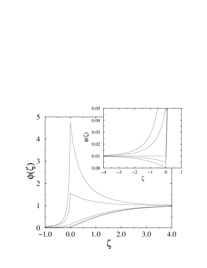
Figure 1: Reduced order parameter profile $\phi=\varphi(z)/\varphi_{b}^{\scriptscriptstyle+}$ at the $\varphi^{3}-\varphi^{4}$ interface as a function of $\zeta=z/\xi_{\scriptscriptstyle+}$ for different values of $\lambda=\Lambda/\xi_{0}^{\scriptscriptstyle+}$ with $1/\lambda=-0.2$, $-0.1$, 0, $0.1$ and $0.5$, from top to bottom. The behavior for $\lambda\geq 0$ and $\zeta<0$ is enlarged in the inset where $1/\lambda=0$, $0.1$, $0.5$, $1$ and $10$, from top to bottom. One may notice the change of behavior at $1/\lambda_{c}=\xi_{0}^{\scriptscriptstyle+}/\Lambda_{c}=1/2$. All other parameters have the same values in the two subsystems: $C\!_{\scriptscriptstyle+}=C\!_{\scriptscriptstyle-}=C_{i}$, $\varphi_{0}^{\scriptscriptstyle+}=\varphi_{0}^{\scriptscriptstyle-}$, $\xi_{0}^{\scriptscriptstyle+}=\xi_{0}^{\scriptscriptstyle-}$ and $t=10^{-4}$.

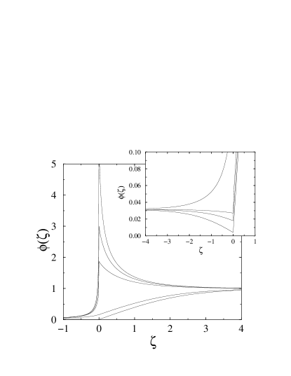
Figure 2: Reduced order parameter profile $\phi=\varphi(z)/\varphi_{b}^{\scriptscriptstyle+}$ at the $\varphi^{4}-\varphi^{6}$ interface as a function of $\zeta=z/\xi_{\scriptscriptstyle+}$ for different values of $\lambda=\Lambda/\xi_{0}^{\scriptscriptstyle+}$ with $1/\lambda=-0.1$, $-0.05$, $-0.03$, $0$ and $0.1$, from top to bottom. The behavior for $\lambda\geq 0$ and $\zeta<0$ is enlarged in the inset where $1/\lambda=0$, $0.01$, $0.02$ and $0.1$, from top to bottom. All other parameters have the same values in the two subsystems and $t=10^{-6}$.

$c$. $\Lambda\to\infty$. The profile remains monotonously increasing and keeps the same functional form as for $\Lambda>\Lambda_{c}$ although $l_{\scriptscriptstyle-}$ and $l_{\scriptscriptstyle+}$ are now given by

$$l_{\scriptscriptstyle-} = 2\left(3\frac{C\!_{\scriptscriptstyle-}\varphi_{0}^{\scriptscriptstyle-}}{C\!_{\scriptscriptstyle+}\varphi_{0}^{\scriptscriptstyle+}}\xi_{0}^{\scriptscriptstyle+}\right)^{1/3}(\xi_{0}^{\scriptscriptstyle-})^{2/3}t^{-1/3}\,,$$

$$l_{\scriptscriptstyle+} = \left(3\frac{\varphi_{0}^{\scriptscriptstyle-}}{\varphi_{0}^{\scriptscriptstyle+}}\xi_{0}^{\scriptscriptstyle+}\right)^{1/3}\left(\frac{C\!_{\scriptscriptstyle+}}{C\!_{\scriptscriptstyle-}}\xi_{0}^{\scriptscriptstyle-}\right)^{2/3}t^{-1/3}\,,$$ (47)

so that

$$\varphi(0)=\frac{1}{2}\left(3\varphi_{0}^{\scriptscriptstyle-}\right)^{1/3}\left(\frac{C\!_{\scriptscriptstyle+}\xi_{0}^{\scriptscriptstyle-}}{C\!_{\scriptscriptstyle-}\xi_{0}^{\scriptscriptstyle+}}\varphi_{0}^{\scriptscriptstyle+}\right)^{2/3}t^{2/3}\,.$$ (48)

II.3.2 $\varphi^{4}-\varphi^{6}$ interface

$a$. $\Lambda<0$. The interface is more ordered than the bulk. Thus $\varphi_{\scriptscriptstyle-}(z)$ is given by (18) and $\varphi_{\scriptscriptstyle+}(z)$ by (20) with

$$l_{\scriptscriptstyle-} = \frac{f}{2}\frac{C\!_{\scriptscriptstyle-}}{C_{i}}|\Lambda|\,,$$

$$l_{\scriptscriptstyle+} = 2\left[\tanh^{-1}\left(\frac{1}{\sqrt{3}}\right)+h(t)\right]\xi_{0}^{\scriptscriptstyle+}t^{-1/2}\,,$$

$$h(t) = \frac{\sqrt{3}}{32}\left(\frac{C\!_{\scriptscriptstyle-}\varphi_{0}^{\scriptscriptstyle+}|\Lambda|}{C_{i}\varphi_{0}^{\scriptscriptstyle-}\xi_{0}^{\scriptscriptstyle-}}f\right)^{2}t^{1/2}\,,$$ (49)

where

$$f=1+\sqrt{1+\frac{8}{\sqrt{3}}\frac{\Lambda^{*}}{|\Lambda|}}\,,\quad\Lambda^{*}=\frac{C_{i}C\!_{\scriptscriptstyle+}(\varphi_{0}^{\scriptscriptstyle-}\xi_{0}^{\scriptscriptstyle-})^{2}}{(C\!_{\scriptscriptstyle-}\varphi_{0}^{\scriptscriptstyle+})^{2}\xi_{0}^{\scriptscriptstyle+}}$$ (50)

Here and below in Eq. (57) we keep the next-to-leading term $h(t)$ in $l_{\scriptscriptstyle+}$. This correction is actually needed to obtain the correct form of the profile in the vicinity of $z=0$. The leading contribution to the order parameter at the interface is constant:

$$\varphi(0)=\frac{4}{f}\frac{C_{i}\xi_{0}^{\scriptscriptstyle-}}{C\!_{\scriptscriptstyle-}|\Lambda|}\varphi_{0}^{\scriptscriptstyle-}\,.$$ (51)

Its asymptotic behavior

$$\varphi(0)\propto\left\{\begin{array}[]{ll}|\Lambda|^{-1}&|\Lambda|\gg\Lambda^{*}\\ |\Lambda|^{-1/2}&|\Lambda|\ll\Lambda^{*}\\ \end{array}\right.\,,$$ (52)

follows from Eqs. (50) and (51)

$b$. $\Lambda>0$. The profile is always decreasing when the interface is approached. Thus $\varphi_{\scriptscriptstyle-}(z)$ is given by (19) and $\varphi_{\scriptscriptstyle+}(z)$ by (21) with the following expressions for the integration constants:

$$l_{\scriptscriptstyle-} = \sqrt{\frac{2}{3}}\frac{C\!_{\scriptscriptstyle+}\varphi_{0}^{\scriptscriptstyle+}\xi_{0}^{\scriptscriptstyle-}}{C_{i}\varphi_{0}^{\scriptscriptstyle-}\xi_{0}^{\scriptscriptstyle+}}\Lambda t^{-1/4}\,,$$

$$l_{\scriptscriptstyle+} = \frac{C\!_{\scriptscriptstyle+}}{C_{i}}\Lambda\,.$$ (53)

The interface order parameter behaves as

$$\varphi(0)=\frac{1}{\sqrt{6}}\frac{C\!_{\scriptscriptstyle+}\Lambda}{C_{i}\xi_{0}^{\scriptscriptstyle+}}\varphi_{0}^{\scriptscriptstyle+}t^{3/4}\,.$$ (54)

$c$. $\Lambda\to\infty$.

Then the profile increases monotonously with $z$. $\varphi_{\scriptscriptstyle-}(z)$ is given by (18) and $\varphi_{\scriptscriptstyle+}(z)$ by (21) with

$$l_{\scriptscriptstyle-} = \left(2\sqrt{6}\frac{C\!_{\scriptscriptstyle-}\varphi_{0}^{\scriptscriptstyle-}}{C\!_{\scriptscriptstyle+}\varphi_{0}^{\scriptscriptstyle+}}\xi_{0}^{\scriptscriptstyle-}\xi_{0}^{\scriptscriptstyle+}\right)^{1/2}t^{-3/8}\,,$$

$$l_{\scriptscriptstyle+} = \left(2\sqrt{6}\frac{C\!_{\scriptscriptstyle+}\varphi_{0}^{\scriptscriptstyle-}}{C\!_{\scriptscriptstyle-}\varphi_{0}^{\scriptscriptstyle+}}\xi_{0}^{\scriptscriptstyle-}\xi_{0}^{\scriptscriptstyle+}\right)^{1/2}t^{-3/8}\,.$$ (55)

The interface order parameter vanishes as

$$\varphi(0)=\left(\sqrt{\frac{2}{3}}\frac{C\!_{\scriptscriptstyle+}\xi_{0}^{\scriptscriptstyle-}}{C\!_{\scriptscriptstyle-}\xi_{0}^{\scriptscriptstyle+}}\varphi_{0}^{\scriptscriptstyle-}\varphi_{0}^{\scriptscriptstyle+}\right)^{1/2}t^{3/8}\,.$$ (56)

II.3.3 $\varphi^{3}-\varphi^{6}$ interface

$a$. $\Lambda<0$. As usual in this case, the interface is more ordered than the bulk. The profiles, $\varphi_{\scriptscriptstyle-}(z)$ and $\varphi_{\scriptscriptstyle+}(z)$ are given by Eqs. (16) and (20). The calculation of $l_{\scriptscriptstyle-}$ involves the solution of an equation of the fourth degree (see Appendix B). Here we only report the limiting behavior for large and small values of $|\Lambda|$:

$$l_{\scriptscriptstyle-} \sim 2\frac{C\!_{\scriptscriptstyle-}}{C_{i}}|\Lambda|\,,\qquad|\Lambda|\gg\Lambda^{*}\,,$$

$$l_{\scriptscriptstyle-} \sim \!\!\left(2\sqrt{27}\frac{C\!_{\scriptscriptstyle+}|\Lambda|}{C_{i}\xi_{0}^{\scriptscriptstyle+}}\right)^{1/4}\!\!\!\left(\frac{\varphi_{0}^{\scriptscriptstyle-}}{\varphi_{0}^{\scriptscriptstyle+}}\right)^{1/2}\!\!\!\!\xi_{0}^{\scriptscriptstyle-}\,,\quad|\Lambda|\ll\Lambda^{*}\,,$$

$$l_{\scriptscriptstyle+} = 2\left[\tanh^{-1}\left(\frac{1}{\sqrt{3}}\right)+h(t)\right]\xi_{0}^{\scriptscriptstyle+}t^{-1/2}\,,$$

$$h(t) = \frac{2\sqrt{3}}{9}\left(\frac{C\!_{\scriptscriptstyle-}|\Lambda|}{C_{i}\xi_{0}^{\scriptscriptstyle-}}\right)^{4}\left(\frac{\varphi_{0}^{\scriptscriptstyle+}}{\varphi_{0}^{\scriptscriptstyle-}}\right)^{2}t^{1/2}\,,\quad|\Lambda|\gg\Lambda^{*}\,,$$

$$h(t) = \frac{1}{4}\frac{C\!_{\scriptscriptstyle+}|\Lambda|}{C_{i}\xi_{0}^{\scriptscriptstyle+}}\,t^{1/2}\,,\qquad|\Lambda|\ll\Lambda^{*}\,.$$ (57)

The crossover is taking place around

$$\Lambda^{*}=C_{i}\left(\frac{\varphi_{0}^{\scriptscriptstyle-}}{\varphi_{0}^{\scriptscriptstyle+}}\right)^{2/3}\left(\frac{C\!_{\scriptscriptstyle+}}{\xi_{0}^{\scriptscriptstyle+}}\right)^{1/3}\left(\frac{\xi_{0}^{\scriptscriptstyle-}}{C\!_{\scriptscriptstyle-}}\right)^{4/3}\,.$$ (58)

The interface order parameter reads

$$\varphi(0) \sim \frac{3}{2}\left(\frac{C_{i}\xi_{0}^{\scriptscriptstyle-}}{C\!_{\scriptscriptstyle-}\Lambda}\right)^{2}\varphi_{0}^{\scriptscriptstyle-}\,,\qquad|\Lambda|\gg\Lambda^{*}\,,$$

$$\varphi(0) \sim \left(2\sqrt{3}\frac{C_{i}\xi_{0}^{\scriptscriptstyle+}}{C\!_{\scriptscriptstyle+}|\Lambda|}\right)^{1/2}\varphi_{0}^{\scriptscriptstyle+}\,,\qquad|\Lambda|\ll\Lambda^{*}\,,$$ (59)

Figure 3: Reduced order parameter profile $\phi=\varphi(z)/\varphi_{b}^{\scriptscriptstyle+}$ at the $\varphi^{3}-\varphi^{6}$ interface as a function of $\zeta=z/\xi_{\scriptscriptstyle+}$ for different values of $\lambda=\Lambda/\xi_{0}^{\scriptscriptstyle+}$ with $1/\lambda=-0.2$, $-0.05$, $-0.02$, $0$ and $1$, from top to bottom. The behavior for $\lambda\geq 0$ and $\zeta<0$ is enlarged in the inset where $1/\lambda=0$, $0.2$, $0.5$, $1$ and $10$, from top to bottom. All other parameters have the same values in the two subsystems and $t=10^{-3}$.

$b$. $\Lambda>0$. The profile is monotonously increasing. $\varphi_{\scriptscriptstyle-}(z)$ and $\varphi_{\scriptscriptstyle+}(z)$ have the form given in Eqs. (16) and (21) with the following values of the constants:

$$l_{\scriptscriptstyle-} = \left(6\sqrt{6}\frac{C_{i}\varphi_{0}^{\scriptscriptstyle-}\xi_{0}^{\scriptscriptstyle+}}{C\!_{\scriptscriptstyle+}\varphi_{0}^{\scriptscriptstyle+}\Lambda}\right)^{1/2}\xi_{0}^{\scriptscriptstyle-}t^{-3/8}\,,$$

$$l_{\scriptscriptstyle+} = \frac{C\!_{\scriptscriptstyle+}}{C_{i}}\Lambda\,.$$ (60)

The interface order parameter vanishes as

$$\varphi(0)=\frac{1}{\sqrt{6}}\frac{C\!_{\scriptscriptstyle+}\Lambda}{C_{i}\xi_{0}^{\scriptscriptstyle+}}\varphi_{0}^{\scriptscriptstyle+}t^{3/4}\,.$$ (61)

$c$. $\Lambda\to\infty$. The profile is still given by Eqs. (16) and (21) with the following values of the constants:

$$l_{\scriptscriptstyle-} = \left[12\sqrt{6}\frac{C\!_{\scriptscriptstyle-}\varphi_{0}^{\scriptscriptstyle-}}{C\!_{\scriptscriptstyle+}\varphi_{0}^{\scriptscriptstyle+}}(\xi_{0}^{\scriptscriptstyle-})^{2}\xi_{0}^{\scriptscriptstyle+}\right]^{1/3}t^{-1/4}\,,$$

$$l_{\scriptscriptstyle+} = \sqrt{6}\left(\frac{1}{2}\frac{C\!_{\scriptscriptstyle+}}{C\!_{\scriptscriptstyle-}}\right)^{2/3}\left[\frac{\varphi_{0}^{\scriptscriptstyle-}}{\varphi_{0}^{\scriptscriptstyle+}}(\xi_{0}^{\scriptscriptstyle-})^{2}\xi_{0}^{\scriptscriptstyle+}\right]^{1/3}t^{-1/4}\,.$$ (62)

At the interface we obtain

$$\varphi(0)=\left(\frac{1}{2}\frac{C\!_{\scriptscriptstyle+}\xi_{0}^{\scriptscriptstyle-}}{C\!_{\scriptscriptstyle-}\xi_{0}^{\scriptscriptstyle+}}\varphi_{0}^{\scriptscriptstyle+}\right)^{2/3}(\varphi_{0}^{\scriptscriptstyle-})^{1/3}t^{1/2}\,.$$ (63)

III Scaling considerations

Here we generalize the mean-field results obtained in the previous section. First, we consider the order-parameter profiles in semi-infinite systems with free and fixed boundary conditions. These results are used afterwards to study the scaling behavior at an interface, which separates two different semi-infinite systems.

III.1 Order-parameter profiles in semi-infinite systems

We consider a semi-infinite system, which is located in the half-space $z>0$, and which is in its bulk-ordered phase ($T\leq T_{c}$); see in Sec. II.2. As in mean-field theory, the order-parameter $\varphi(z)$ depends on the distance from the surface, $z$, and approaches its bulk value, $\varphi_{b}\sim t^{\beta}$, for $z/\xi\gg 1$. The bulk correlation length asymptotically behaves as $\xi\sim|t|^{-\nu}$. These expressions generalize the mean-field results in Eqs. (9) and (13).

III.1.1 Free boundary conditions

At a free surface, due to the missing bonds the local order is weaker than in the bulk. The surface order parameter displays the so-called ordinary transition with the temperature dependence $\varphi(0)\sim t^{\beta_{1}}$, where generally $\beta_{1}>\beta$. The profile, $\varphi(z)$, which interpolates between the surface and the bulk value has the scaling formbinder83 ; diehl86 ; pleimling04

$$\varphi(z)=\varphi_{b}f_{\rm ord}\left(\frac{z+l}{\xi}\right)\;,$$ (64)

and the scaling function, $f_{\rm ord}(y)$, behaves as $y^{(\beta_{1}-\beta)/\nu}$, for $y\ll 1$.

III.1.2 Fixed boundary conditions

For fixed boundary conditions, the system displays the extraordinary surface transition and stays ordered in the surface region at the bulk critical temperature, so that $\varphi(z)=O(1)$ as $t\to 0_{\scriptscriptstyle+}$ and $z\ll\xi$. This behavior is formally equivalent to having a surface exponent, $\beta_{1}=0$. The magnetization profile can be written into an analogous formbinder83 ; diehl86 ; pleimling04 as in Eq. (64):

$$\varphi(z)=\varphi_{b}f_{\rm ext}\left(\frac{z+l}{\xi}\right)\;,$$ (65)

however, now the scaling function, $f_{\rm ext}(y)$ has the asymptotic behavior,fisher78 $f_{\rm ext}(y)\sim y^{-\beta/\nu}$, for $y\ll 1$.

III.2 Interface critical behavior

Now we join the two semi-infinite systems and study the behavior of the order-parameter in the vicinity of the interface. In general we expect that, depending on the strength of the interface coupling, at the bulk critical temperature the interface (i) can stay disordered for weak couplings, which corresponds to the $\Lambda>0$ case in mean-field theory or (ii) can stay ordered for stronger couplings, which is the case for $\Lambda<0$ in mean-field theory. These two regimes of interface criticality are expected to be separated by a special transition point, which corresponds to $\Lambda\to\infty$ in mean-field theory.

To construct the order-parameter profile we start with the profiles in the semi-infinite systems and join them. First we require continuous behavior of the profile at $z=0$, like in mean-field theory. The second condition in mean-field theory in Eq. (38) cannot be directly translated; here we just use its consequencies for the extrapolation lengths. In the weak- and strong-coupling regimes in mean-field theory the left-hand side of Eq. (38) is finite so that the derivative of the profile is discontinuous at $z=0$ and at least one of the extrapolation lengths $l_{\scriptscriptstyle\pm}$ is $O(1)$. The same behavior of $l_{\scriptscriptstyle\pm}$ is expected to hold in scaling theory, too. On the other hand, at the special transition point in mean-field theory the left-hand side of Eq. (38) is zero and the extrapolation lengths are divergent. In scaling theory the asymptotic form of the extrapolation lengths is expected to be deduced from the same condition— i.e. from the equality of the derivatives of the profiles. This leads to a relation $l_{\scriptscriptstyle\pm}\sim t^{-\nu_{\scriptscriptstyle\pm}\omega_{\scriptscriptstyle\pm}}$, in which $0\leq\omega_{\scriptscriptstyle\pm}\leq 1$ is defined later.

If the subsystem—say at $z>0$—has an ordinary transition the interface magnetization follows from Eq. (64) as

$$\varphi(0)\sim t^{\beta_{i}},\quad\beta_{i}=(1-\omega_{\scriptscriptstyle+})\beta_{1}^{\scriptscriptstyle+}+\omega_{\scriptscriptstyle+}\beta_{\scriptscriptstyle+}\;,$$ (66)

and $\beta_{\scriptscriptstyle+}\leq\beta_{i}\leq\beta_{1}^{\scriptscriptstyle+}$. On the other hand, if the subsystem—say at $z<0$—has an extraordinary transition the interface magnetization exponent follows from Eq. (65) as

$$\beta_{i}=\omega_{\scriptscriptstyle-}\beta_{\scriptscriptstyle-}\;.$$ (67)

Evidently, $\beta_{i}$ calculated form the two joined subsystems should have the same value. This type of construction of the order-parameter profiles will lead to a smooth profile at the interface provided the extrapolation lengths are smaller or, at most, of the same order than the correlation lengths, ${\rm max}(l_{\scriptscriptstyle+},l_{\scriptscriptstyle-})\lesssim{\rm min}(\xi_{\scriptscriptstyle+},\xi_{\scriptscriptstyle-})$, which holds provided

$${\rm max}(\omega_{\scriptscriptstyle+}\nu_{\scriptscriptstyle+},\omega_{\scriptscriptstyle-}\nu_{\scriptscriptstyle-})\leq{\rm min}(\nu_{\scriptscriptstyle+},\nu_{\scriptscriptstyle-})\;.$$ (68)

Otherwise, the profile measured in a length scale, ${\rm min}(\xi_{\scriptscriptstyle+},\xi_{\scriptscriptstyle-})$, has a sharp variation at the interface and as the critical temperature is approached the profile becomes discontinuous. Note that in mean-field theory, with $\nu_{\scriptscriptstyle+}=\nu_{\scriptscriptstyle-}$ and $\omega_{\scriptscriptstyle\pm}\leq 1$, the profile is always smooth.

III.2.1 Relevance-irrelevance criterion

Here we generalize the relevance-irrelevance criterion known to hold at an internal defect plane with weak defect couplings.burkhardt81 If two different critical systems are weakly coupled, the operator corresponding to the junction is the product of the two surface magnetization operators. Consequently, its anomalous dimension $x_{i}$ is given by the sum of the dimensions of the two surface operators, $x_{i}=x_{1}^{\scriptscriptstyle-}+x_{1}^{\scriptscriptstyle+}$, where $x_{1}^{\scriptscriptstyle\pm}=\beta_{1}^{\scriptscriptstyle\pm}/\nu_{\scriptscriptstyle\pm}$. Then the scaling exponent of the defect, $y_{i}$, in a $d$-dimensional system is given by

$$y_{i}=d_{i}-x_{i}=d-1-\frac{\beta_{1}^{\scriptscriptstyle+}}{\nu_{\scriptscriptstyle+}}-\frac{\beta_{1}^{\scriptscriptstyle-}}{\nu_{\scriptscriptstyle-}}\;.$$ (69)

where $d_{i}=d-1$ is the dimension of the interface.

For $y_{i}<0$ the weak interface coupling is irrelevant so that the defect coupling renormalizes to zero and the defect acts as a cut in the system. Consequently the interface critical behavior is the same as in the uncoupled semi-infinite systems and the interface magnetization exponent is $\beta_{i}={\rm min}(\beta_{1}^{\scriptscriptstyle\pm})$ since the stronger local order manifests itself at the interface. In the other case, $y_{i}>0$, the coupling at the interface is relevant and the interface critical behavior is expected to be controlled by a new fixed point.

For the 2D $q$-state Potts model with $2\leq q\leq 4$ we havecardy84 $x_{1}\geq 1/2$; thus weak interface coupling is expected to be irrelevant according to Eq. (69).

In mean-field theory, when $d$ appears in a scaling relation, it has to be replaced by the upper critical dimension $d_{c}$ for which hyperscaling is verified. However we have here different values of $d_{c}$ for the two subsystems so that there is some ambiguity for the value of $d$ in Eq. (69). The analytical results of Sec. II.3 show that a weak interface coupling is also irrelevant in all the cases studied in mean-field theory.

III.2.2 Weakly coupled systems

For weak interface coupling the order parameter profile is not expected to display a maximum at the interface. Depending on the relative values of the critical exponents, $\beta_{\scriptscriptstyle+},~{}\beta_{\scriptscriptstyle-},~{}\beta_{1}^{\scriptscriptstyle+},~{}\beta_{1}^{\scriptscriptstyle-}$ it can be either a minimum, or an intermediate point of a monotonously increasing profile. We use the same convention as in Sec. II.3, that $\beta^{\scriptscriptstyle+}<\beta^{\scriptscriptstyle-}$ and treat separately the different cases.

$a$. $\beta_{\scriptscriptstyle+}<\beta_{\scriptscriptstyle-}<\beta_{1}^{\scriptscriptstyle+}<\beta_{1}^{\scriptscriptstyle-}$. The order-parameter profile is obtained by joining two ordinary surface profiles in Eq. (64) both for $z<0$ and for $z>0$. In this case the weak coupling does not modify the asymptotic behavior of the more ordered, $z>0$ subsystem. Consequently we have $\varphi(0)\sim\varphi_{1}^{\scriptscriptstyle+}$, $l_{\scriptscriptstyle+}=O(1)$ and $\omega_{\scriptscriptstyle+}=0$; thus $\beta_{i}=\beta_{1}^{\scriptscriptstyle+}$. From Eq. (66) we obtain

$$\omega_{\scriptscriptstyle-}=\frac{\beta_{1}^{\scriptscriptstyle-}-\beta_{1}^{\scriptscriptstyle+}}{\beta_{1}^{\scriptscriptstyle-}-\beta_{\scriptscriptstyle-}}\;.$$ (70)

Note that the above reasoning leads to a smooth order-parameter profile at the interface, if according to Eq. (68) we have $\omega_{\scriptscriptstyle-}\nu_{\scriptscriptstyle-}<\nu_{\scriptscriptstyle+}$. This type of behavior is realized in mean-field theory for the $\varphi^{4}-\varphi^{6}$ interface for $\Lambda>0$, see in Sec. II.3.2.

$b$. $\beta_{\scriptscriptstyle+}<\beta_{\scriptscriptstyle-}<\beta_{1}^{\scriptscriptstyle-}<\beta_{1}^{\scriptscriptstyle+}$. In this case the profile is obtained from two ordinary subprofiles. The order parameter is still minimum at the interface, but it is determined by the $z<0$ subsystem, which has the larger surface order parameter. Consequently, $\varphi(0)\sim\varphi_{1}^{\scriptscriptstyle-}$, $l_{\scriptscriptstyle-}=O(1)$ and $\omega_{\scriptscriptstyle-}=0$; thus $\beta_{i}=\beta_{1}^{\scriptscriptstyle-}$. From Eq. (66) we obtain

$$\omega_{\scriptscriptstyle+}=\frac{\beta_{1}^{\scriptscriptstyle+}-\beta_{1}^{\scriptscriptstyle-}}{\beta_{1}^{\scriptscriptstyle+}-\beta_{\scriptscriptstyle+}}\;.$$ (71)

and the order-parameter profile is smooth if $\omega_{\scriptscriptstyle+}\nu_{\scriptscriptstyle+}<\nu_{\scriptscriptstyle-}$. This type of behavior is never realized in mean-field theory; see the exponent relation in Eq. (35).

$c$. $\beta_{\scriptscriptstyle+}<\beta_{1}^{\scriptscriptstyle+}<\beta_{\scriptscriptstyle-}<\beta_{1}^{\scriptscriptstyle-}$. In this case the order-parameter profile is monotonously increasing and obtained by joining an extraordinary profile in Eq. (65) for $z<0$ with an ordinary profile in Eq. (64) for $z>0$. The order parameter at the interface is determined by the surface order parameter of the $z>0$ subsystem. Then we have $\varphi(0)\sim\varphi_{1}^{\scriptscriptstyle+}$, $l_{\scriptscriptstyle+}=O(1)$ and $\omega_{\scriptscriptstyle+}=0$; thus $\beta_{i}=\beta_{1}^{\scriptscriptstyle+}$. From Eq. (66) we obtain $\omega_{\scriptscriptstyle-}=\beta_{1}^{\scriptscriptstyle+}/\beta_{\scriptscriptstyle-}$ and the interface is smooth, provided $\omega_{\scriptscriptstyle-}\nu_{\scriptscriptstyle-}<\nu_{\scriptscriptstyle+}$. In mean-field theory this type of behavior is realized for the $\varphi^{3}-\varphi^{6}$ interface for $\Lambda>0$; see in Sec. II.3.3.

III.2.3 Special transition point

In this case the profile is monotonously increasing and it is constructed by joining an extraordinary subprofile in Eq. (65) for $z<0$ with an ordinary subprofile in Eq. (64) for $z>0$. As we argued before, the extrapolation lengths and the corresponding exponents are obtained (i) from the continuity of the profile at $z=0$,

$$\beta_{i}=\beta_{\scriptscriptstyle-}\omega_{\scriptscriptstyle-}=(1-\omega_{\scriptscriptstyle+})\beta_{1}^{\scriptscriptstyle+}+\beta_{\scriptscriptstyle+}\omega_{\scriptscriptstyle+}\;,$$ (72)

and (ii) from the continuity of the derivative at $z=0$, which leads to the condition $l_{\scriptscriptstyle+}\sim l_{\scriptscriptstyle-}$—consequently,

$$\nu_{i}=\omega_{\scriptscriptstyle+}\nu_{\scriptscriptstyle+}=\omega_{\scriptscriptstyle-}\nu_{\scriptscriptstyle-}\;.$$ (73)

The solution of Eqs. (72) and (73) is given by

$$\nu_{i}=\frac{\beta_{1}^{\scriptscriptstyle+}}{\frac{\beta_{1}^{\scriptscriptstyle+}-\beta_{\scriptscriptstyle+}}{\nu_{\scriptscriptstyle+}}+\frac{\beta_{\scriptscriptstyle-}}{\nu_{\scriptscriptstyle-}}},\quad\beta_{i}=\frac{\beta_{\scriptscriptstyle-}}{\nu_{\scriptscriptstyle-}}\nu_{i}\;.$$ (74)

Let us now analyze the condition for the smooth or discontinuous nature of the interface given in Eq. (68).

$a$. $\nu_{\scriptscriptstyle-}\geq\nu_{\scriptscriptstyle+}$. In this case the condition is equivalent to $\beta_{\scriptscriptstyle-}/\nu_{\scriptscriptstyle-}>\beta_{\scriptscriptstyle+}/\nu_{\scriptscriptstyle+}$. As we will discuss in Sec. IV this condition is satisfied in 2D for the three- and the four-state Potts (or BW) models so that the profile is predicted to be smooth. On the contrary for the Ising and the three-state Potts models this condition does not hold; thus, the profile is probably sharp and becomes discontinuous at the critical temperature. Finally, for the Ising and the BW models the relation in Eq. (68) is just an equality, so that we are in a marginal situation.

$b$. $\nu_{\scriptscriptstyle-}<\nu_{\scriptscriptstyle+}$. In this case the profile is smooth, provided

$$\beta_{1}^{\scriptscriptstyle+}<\frac{\frac{\beta_{\scriptscriptstyle-}}{\nu_{\scriptscriptstyle-}}-\frac{\beta_{\scriptscriptstyle+}}{\nu_{\scriptscriptstyle+}}}{\frac{1}{\nu_{\scriptscriptstyle-}}-\frac{1}{\nu_{\scriptscriptstyle+}}}\;.$$ (75)

This type of situation seems to be less common in real systems.

III.2.4 Strongly coupled systems

In this case the interface stays ordered at the bulk critical temperature, so that the profile is expected to be composed from two extraordinary subprofiles. As a consequence the interface critical behavior is the same as in two independent semi-infinite systems, both having an extraordinary surface transition.

IV Numerical investigations

We have studied numerically the critical behavior at the interface between two $q$-state Potts models on the square lattice, with different values of $q$ for the two subsystems. For a review of the Potts model, see Ref. wu82, . In particular we considered the value $q=2$, which corresponds the Ising model, as well as $q=3$ and $q=4$. All these systems display a second-order phase transition for a value of the coupling given by $e^{qK_{c}}=1+\sqrt{q}$, which follows from self-duality. The associated critical exponents are exactly knownbaxter82 for $q=2$ ($\beta=1/8$, $\nu=1$ and $\beta_{1}=1/2$) and has been conjectured for $q=3$ ($\beta=1/9$, $\nu=5/6$ and $\beta_{1}=5/9$) and $q=4$ ($\beta=1/12$, $\nu=2/3$ and $\beta_{1}=2/3$), where they follow from conformal invariancecardy87 and the Coulomb-gas mapping.nienhuis87 We have also considered the BW model,baxterwu which is a triangular lattice Ising model with three-spin interactions on all the triangular faces. This model is also self-dual and has the same critical coupling as the Ising model. This model is exactly solved,baxter82 and it belongs to the universality class of the $q=4$ state Potts model, but without logarithmic corrections to scaling, which facilitates the analysis of the numerical data.

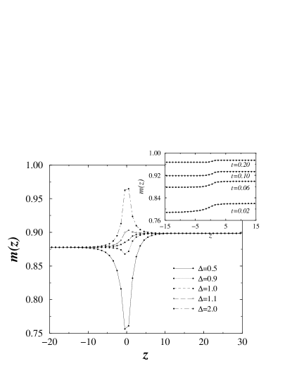
Figure 4: Order parameter profiles of the $q=3-4$ interface at the reduced temperature $t=0.06$ and for different values of the interface coupling ratio, $\Delta=2.0,1.1,1.0,0.9$ and $0.5$ from top to bottom. Inset: profiles around the special transition point, $\Delta=1$, for different temperatures. The results indicate a smooth profile at the transition point.

We have performed Monte Carlo simulations on 2D systems consisting of two $L\times L$ subsystems which interact directly through interface couplings $K_{i}$ (between adjacent spins of the two subsystems) such that $K_{i}/K_{\scriptscriptstyle+}=\Delta$. Here $K_{\scriptscriptstyle+}$ is the coupling in the half-space $z>0$, which corresponds to the subsystem having the larger value of $q$, thus the larger magnetization. Periodic boundary conditions are applied in both directions. Using the Swendsen-Wang cluster-flip algorithmsw we have calculated the magnetization profile in systems with size up to $L=300$ for different values of the reduced temperature $t=(T_{c}-T)/T_{c}$ and coupling ratio $\Delta$. Depending on the size of the system and the temperature we have skipped the first $5-20\times 10^{4}$ thermalization steps and the thermal averages were taken over $6-20\times 10^{6}$ MC steps. We have checked that the magnetization profiles, at the reduced temperatures we used, does not show any noticeable finite-size effects. From the magnetization data at the interface we have calculated effective, temperature-dependent interface exponents given by

$$\beta_{i}(t)=\frac{\log[m(t+\delta)/m(t-\delta)]}{\log[(t+\delta)/(t-\delta)]}\;,$$ (76)

which approach the true exponents as $\delta\to 0$ and $t\to 0$. For the Ising-BW interface, we have also made calculations at the critical temperature in order to check the finite-size scaling properties of the profiles. In the following we present the numerical results for the $q=2-3$, $q=3-4$ and Ising-BW interfaces. In each case we have a different type of special transition, separating the ordinary and the extraordinary transition regimes.

IV.1 $\bm{q=3-4}$ interface

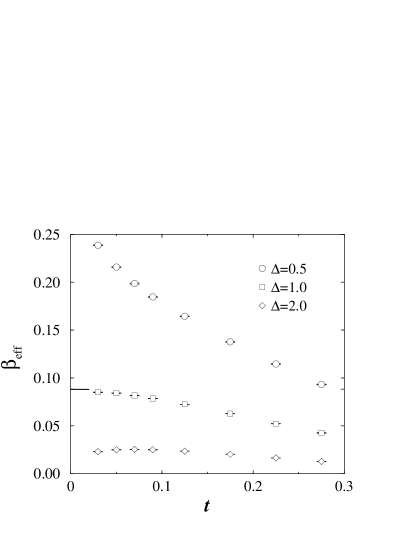
Figure 5: Effective magnetization exponents measured on the two sides of the $q=3-4$ interface for three different values of the coupling ratio, $\Delta$. At the special transition point, $\Delta\approx 1$, the theoretical prediction from Eq. (74) is indicated by a bar.

We start in Fig. 4 with a presentation of the order-parameter profiles, in the vicinity of the critical temperature, for different values of the interface coupling. Here one can differentiate between the ordinary transition regime for small $\Delta$, in which the magnetization at the interface vanishes faster than in the bulk of the two subsystems, and the extraordinary transition regime for large $\Delta$, where the interface magnetization keeps a finite value. The special transition separating these two regimes is located at $\Delta\approx 1$. The inset of Fig. 4 shows the evolution of the interface at the special transition point as the bulk transition point is approached. Here the criterion in Eq. (68) is satisfied, since, as discussed below Eq. (74), $\beta_{\scriptscriptstyle-}/\nu_{\scriptscriptstyle-}=2/15>\beta_{\scriptscriptstyle+}/\nu_{\scriptscriptstyle+}=1/8$. Thus the profile is predicted to be smooth, which is in accordance with the numerical results.

The values of the effective, temperature-dependent exponents, as defined in Eq. (76), are presented in Fig. 5 for three values of $\Delta$, corresponding to the different transition regimes. Clearly the values of the effective exponents are affected by strong crossover effects for small $t$, since the limiting values are $\beta_{i}=\beta_{1}(q=3)=5/9$ for $\Delta<1$ and $\beta_{i}=0$ for $\Delta>1$, according to scaling theory. Unfortunately, due to finite-size effects we could not go closer to the critical point. At the special transition point, however, the crossover effects are weaker and the effective exponents are close to the theoretical prediction in Eq. (74), $\beta_{i}=32/363=0.088$.

IV.2 $\bm{q=2-3}$ interface

Figure 6: The same as in Fig. 4 for the $q=2-3$ interface with interface coupling ratio $\Delta=2.0,1.0,0.9,0.85,0.8$ and $0.5$ from top to bottom and $t=0.06$. Inset: profiles around the special transition point, $\Delta_{c}=0.85$, for different temperatures. The results indicate that the profile becomes discontinuous at the critical temperature.

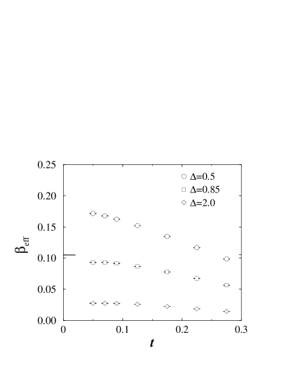
Figure 7: The same as in Fig. 5 for the $q=2-3$ interface.

We have performed a similar investigation for the interface critical behavior of the $q=2-3$ system and the results are summarized in Figs. 6 and 7. Here one can also identify the ordinary and the extraordinary transition regimes (see Fig. 6), which are separated by the special transition around $\Delta\approx 0.85$. However, as can be seen in the inset of Fig. 6, the behavior around the special transition point is more complex than for the $q=2-3$ interface. The evolution of the profile suggests the existence of a discontinuity at the transition temperature. This is in accordance with the scaling criterion in Eq. (68) since, as discussed below Eq. (74), $\beta_{\scriptscriptstyle-}/\nu_{\scriptscriptstyle-}=1/8<\beta_{\scriptscriptstyle+}/\nu_{\scriptscriptstyle+}=2/15$ leads to a discontinuous profile. Due to this discontinuity, it is more difficult to locate precisely the special transition point and to determine the associated interface exponent $\beta_{i}$. The measured effective interface exponents are shown in Fig. 7 for three values of $\Delta$ corresponding to the different interface fixed points. The crossover effects are strong but, at the special transition point, our estimates are compatible with the scaling prediction in Eq. (74), $\beta_{i}=25/237=0.105$.

IV.3 Ising-BW interface

Figure 8: Critical magnetization profiles in the Ising-BW system with two symmetrically placed interfaces for different values of the coupling ratio $\Delta$.

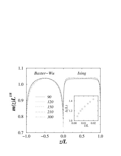
Figure 9: Scaled magnetization profiles for the coupled Ising-BW systems at the common critical temperature for $L=90$ — $300$. The interface coupling ratio is fixed at the critical value, $\Delta_{c}(L)$, for which the two maxima of the curves are identical. The inset gives the effective critical interface coupling as a function of the inverse size.

The interface between the Ising model and the BW model (or the four-state Potts model) has some special features. These are mainly due to the fact that the anomalous dimension of the bulk magnetization in the two systems has the same value, $\beta_{\scriptscriptstyle-}/\nu_{\scriptscriptstyle-}=\beta_{\scriptscriptstyle+}/\nu_{\scriptscriptstyle+}=1/8$. Consequently one can define and numerically study the finite-size scaling properties of the magnetization profile at the phase-transition point, since it is expected to scale as $m(z,L)=L^{-1/8}f(z/L)$. The scaling function $f(y)$ is expected to depend on the value of the interface coupling ratio $\Delta$ and we have studied this quantity numerically.

The magnetization profiles at the critical temperature for different values of the interface coupling ratio $\Delta$ are given in Fig. 8. It is interesting to notice that the shape of the curves as well as the relative heights of the profiles in the two subsystems vary with the interface coupling. For $\Delta<\Delta_{c}\approx 1$, the interface stays disordered and the interface critical behavior is governed by the surface exponent of the Ising model. The larger bulk value on the Ising side is understandable since the profile on the right side is more singular, $\beta_{1}^{\scriptscriptstyle-}/\nu_{\scriptscriptstyle-}>\beta_{1}^{\scriptscriptstyle+}/\nu_{\scriptscriptstyle+}$; see below Eq.(64). On the contrary, for $\Delta>\Delta_{c}$ the interface is ordered at the bulk critical temperature and the profiles decay towards the bulk values.

At the special transition point $\Delta=\Delta_{c}$, the profile has a universal form in terms of $L^{1/8}m(z/L)$. This is illustrated in Fig. 9, in which for each finite system a critical value $\Delta_{c}(L)$ is calculated from the condition that the two maxima of the curves have identical values and the profile is measured at that interface coupling. The size-dependent effective interface coupling ratio, $\Delta_{c}(L)$, shown in the inset of Fig. 9, seems to tend to a limiting value, $\Delta_{c}\approx 1$. The scaled magnetization profiles have different characteristics in the two subsystems. In the BW model, having the smaller correlation length, the profile has a smooth variation. On the contrary, on the Ising side, the profile has a quasidiscontinuous nature at the interface, which is probably related to the fact that in the criterion of Eq. (68) the equality holds.

V Discussion

In this paper we have studied the critical behavior at the interface between two subsystems displaying a second-order phase transition. We assumed that the critical temperatures are identical but the sets of critical exponents (i.e., the universality classes of the transitions) are different for the two subsystems. By varying the interface couplings, we monitored the order at the interface and studied the behavior of the order-parameter profile as the critical temperature is approached. We provided a detailed analytical solution of the problem in the framework of mean-field theory, which leads to a physical picture which is useful for the study of realistic systems. Solutions of the mean-field equations are obtained by adjusting the order-parameter profiles of the two semi-infinite subsystems through the introduction of appropriate extrapolation lengths on the two sides. The same strategy has been applied in the frame of a phenomenological scaling approach. As a result, basically three types of interface critical behavior are observed. For weak interface couplings the interface renormalizes to an effective cut and we are left with the surface critical behavior of the subsystems. In the limit of strong interface couplings, the renormalization leads to infinitely strong local couplings and thus interface order at the bulk critical point. Finally, for some intermediate value of the interface couplings, the interface displays a special transition, which is characterized by a new critical exponent for the order parameter in the interface region. In the scaling theory this exponent can be expressed in terms of the bulk and surface exponents of the semi-infinite subsystems.

These results have been tested through large scale Monte Carlo simulations, in which the critical behavior at the interface between 2D Ising, Potts and BW models was studied and satisfactory agreement has been found. However, it would be interesting to confirm the analytical expressions for the interface exponents through a field-theoretical renormalization group study, using the methods of Ref. diehl86, .

The results obtained in this paper can be generalized into different directions. First we mention the case when the critical temperatures of the subsystems are not exactly equal but differ by an amount, $\Delta T_{c}$. If the deviation in temperature from the average value, $\overline{T}_{c}=(T_{c}^{\scriptscriptstyle-}+T_{c}^{\scriptscriptstyle+})/2$, is small but satisfies $\overline{T}_{c}-T\gg\Delta T_{c}$, then our results are still valid. Our second remark concerns 3D systems in which sufficiently enhanced interface couplings may lead to an independent ordering of the interface above the bulk critical temperatures. In semi-infinite systems this phenomena is called the surface transition.binder83 ; diehl86 ; pleimling04 At the bulk critical temperature the ordered interface then shows a singularity, which is analogous to the extraordinary transition in semi-infinite systems. The singularities at the interface and extraordinary interface transitions remain to be determined, even in the mean-field approach. Third, we can mention that non-trivial interface critical behavior could be observed when one of the subsystems displays a first-order transition. It is known for semi-infinite systems that the surface may undergo a continuous transition, which, however, has an anisotropic scaling character, even if the bulk transition is discontinuous.lipowsky84 ; ti02 Similar phenomena can happen at an interface, too. Our final remark concerns the localization-delocalization transition of the interface provided an external ordering field is applied. For two subsystems having the same $\varphi^{4}$ mean-field theory and the samesevrin89 or differentigloi90 critical temperatures, this wetting problem has already been solved. This solution could be generalized for subsystems having different field-theoretical descriptions.

Appendix A Surface critical behavior

The calculation of the surface behavior is straightforward when $l/\xi\to 0$ at the critical point. Here we give some details about the two cases where the surface boundary condition leads to a constant value for $l/\xi$.

A.1 $\bm{\varphi^{3}}$ model with $\bm{\Lambda>0}$

Using the results of Eq. (17), the boundary condition in (22) is rewritten as

$$\frac{C_{s}}{2\Lambda}\!\left[3\tanh^{2}\!\left(\!\frac{l}{2\xi}\!\right)\!\!-\!\!1\right]\!\!=\!\frac{3C}{2\xi}\sinh\!\left(\!\frac{l}{2\xi}\!\right)\!\cosh\!^{-3}\!\left(\!\frac{l}{2\xi}\!\right).$$ (77)

Let

$$3\tanh^{2}\left(\frac{l}{2\xi}\right)-1=\alpha t^{1/2}\,,\quad\hat{\varphi}(0)=\frac{\alpha}{2}t^{1/2}\,.$$ (78)

Then, to leading order

$$\tanh\left(\frac{l}{2\xi}\right)=\frac{1}{\sqrt{3}}\,,\quad\cosh^{-2}\left(\frac{l}{2\xi}\right)=\frac{2}{3}\,.$$ (79)

The first relation gives $l$ in Eq. (25), and (77) leads to

$$\alpha=\frac{2C\Lambda}{\sqrt{3}C_{s}\xi_{0}}$$ (80)

Finally, combining Eqs. (78) and (80), one obtains the value of $\varphi(0)$ given in Eq. (26).

A.2 $\bm{\varphi^{6}}$ model with $\bm{\Lambda<0}$

Since the surface is ordered, the profile is given by Eq. (17). The boundary condition in (22) translates into

$$\frac{\sqrt{2}C_{s}}{|\Lambda|}\left[3\tanh^{2}\left(\frac{l}{2\xi}\right)-1\right]^{-1/2}\!\!\!=\frac{3\sqrt{2}C}{2\xi}\sinh\left(\frac{l}{2\xi}\right)$$

$$\ \ \ \times\cosh^{-3}\left(\frac{l}{2\xi}\right)\left[3\tanh^{2}\left(\frac{l}{2\xi}\right)-1\right]^{-3/2}\!\!\!.$$ (81)

The boundary condition is satisfied when

$$\sqrt{3\tanh^{2}\left(\frac{l}{2\xi}\right)-1}=\alpha t^{1/4}\,,$$ (82)

so that:

$$\hat{\varphi}(0)=\frac{\sqrt{2}}{\alpha}t^{-1/4}\,.$$ (83)

Eq. (82) gives the value of $l$ in Eq. (31). Using the values given in (79) which remain valid here together with Eq. (82) in (81), one obtains:

$$\alpha=\left(\frac{2C|\Lambda|}{\sqrt{3}C_{s}\xi_{0}}\right)^{1/2}\,.$$ (84)

Inserting this expression in (83) leads to the surface order parameter given in Eq. (32).

Appendix B Interface critical behavior

In this Appendix we give some details about the calculations of $l_{\scriptscriptstyle\pm}$ and $\varphi(0)$ limiting ourselves to three representative cases. Other results are easily obtained using similar methods.

B.1 $\bm{l_{\scriptscriptstyle\pm}/\xi_{\scriptscriptstyle\pm}\ll 1}$

This situation is encountered for the $\varphi^{3}-\varphi^{4}$ interface with $\Lambda<0$ and $\Lambda\to\infty$ as well as for the $\varphi^{4}-\varphi^{6}$ and $\varphi^{3}-\varphi^{6}$ interfaces with $\Lambda>0$ and $\Lambda\to\infty$. Here we consider as an example the $\varphi^{3}-\varphi^{4}$ interface with $\Lambda<0$.

The boundary conditions in Eq. (38) are satisfied with $\varphi_{\scriptscriptstyle-}(z)$ and $\varphi_{\scriptscriptstyle+}(z)$ given by (16) and (18) and reads

$$\!\!\!\!\varphi(0)\!=\varphi_{0}^{\scriptscriptstyle+}t^{1/2}\coth\left(\!\frac{l_{\scriptscriptstyle+}}{2\xi_{\scriptscriptstyle+}}\!\right)\!=\!\frac{\varphi_{0}^{\scriptscriptstyle-}t}{2}\left[3\coth^{2}\!\left(\!\frac{l_{\scriptscriptstyle-}}{2\xi_{\scriptscriptstyle-}}\!\right)\!-\!1\right],$$

$$\!\!\!\!\!\!\frac{C\!_{\scriptscriptstyle+}\varphi_{0}^{\scriptscriptstyle+}t^{1/2}}{2\xi_{\scriptscriptstyle+}}\!\sinh^{-2}\!\left(\!\frac{l_{\scriptscriptstyle+}}{2\xi_{\scriptscriptstyle+}}\!\!\right)\!+\!\frac{3C\!_{\scriptscriptstyle-}\varphi_{0}^{\scriptscriptstyle-}t}{2\xi_{\scriptscriptstyle-}}\cosh\!\left(\!\frac{l_{\scriptscriptstyle-}}{2\xi_{\scriptscriptstyle-}}\!\!\right)\!\sinh^{-3}\!\left(\!\frac{l_{\scriptscriptstyle-}}{2\xi_{\scriptscriptstyle-}}\!\!\right)$$

$$\ \ \ \ =\frac{C_{i}\varphi_{0}^{\scriptscriptstyle+}t^{1/2}}{|\Lambda|}\coth\left(\frac{l_{\scriptscriptstyle+}}{2\xi_{\scriptscriptstyle+}}\right)\,.$$ (85)

With $l_{\scriptscriptstyle\pm}/\xi_{\scriptscriptstyle\pm}\ll 1$, one may expand the hyperbolic functions in powers of $l_{\scriptscriptstyle\pm}/(2\xi_{\scriptscriptstyle\pm})$ To leading order, the first equation in (85) gives

$$\varphi(0)=\frac{3\varphi_{0}^{\scriptscriptstyle-}t}{2}\left(\frac{2\xi_{\scriptscriptstyle-}}{l_{\scriptscriptstyle-}}\right)^{2}=\frac{2\varphi_{0}^{\scriptscriptstyle+}\xi_{0}^{\scriptscriptstyle+}}{l_{\scriptscriptstyle+}}\,,$$ (86)

so that

$$\frac{l_{\scriptscriptstyle-}}{2\xi_{\scriptscriptstyle-}}=\sqrt{\frac{3\varphi_{0}^{\scriptscriptstyle-}l_{\scriptscriptstyle+}t}{4\varphi_{0}^{\scriptscriptstyle+}\xi_{0}^{\scriptscriptstyle+}}}\,.$$ (87)

Introducing this result in the second equation, one obtains an equation of the second degree in $x=\sqrt{l_{\scriptscriptstyle+}}$:

$$-x^{2}+2\frac{C\!_{\scriptscriptstyle-}|\Lambda|}{C_{i}\xi_{0}^{\scriptscriptstyle-}}\sqrt{\frac{\varphi_{0}^{\scriptscriptstyle+}\xi_{0}^{\scriptscriptstyle+}}{3\varphi_{0}^{\scriptscriptstyle-}}}x+\frac{C\!_{\scriptscriptstyle+}|\Lambda|}{C_{i}}=0\,.$$ (88)

Thus we have

$$\sqrt{l_{\scriptscriptstyle+}} = f\frac{C\!_{\scriptscriptstyle-}|\Lambda|}{C_{i}\xi_{0}^{\scriptscriptstyle-}}\sqrt{\frac{\varphi_{0}^{\scriptscriptstyle+}\xi_{0}^{\scriptscriptstyle+}}{3\varphi_{0}^{\scriptscriptstyle-}}}\,,$$

$$f = \sqrt{1+3\frac{C\!_{\scriptscriptstyle+}C_{i}\varphi_{0}^{\scriptscriptstyle-}(\xi_{0}^{\scriptscriptstyle-})^{2}}{C_{\scriptscriptstyle-}^{2}\varphi_{0}^{\scriptscriptstyle+}\xi_{0}^{\scriptscriptstyle+}|\Lambda|}}\,.$$ (89)

This last result together with Eqs. (87) and (86) leads to the expressions given in (39) and (41).

B.2 $\bm{l_{\scriptscriptstyle-}/\xi_{\scriptscriptstyle-}}\to$ const., $\bm{l_{\scriptscriptstyle+}/\xi_{\scriptscriptstyle+}\ll 1}$

This behavior is obtained only for the $\varphi^{3}-\varphi^{4}$ interface with $\Lambda>0$. When $\Lambda$ is smaller than a critical value $\Lambda_{c}$ to be determined later, the profiles $\varphi_{\scriptscriptstyle-}(z)$ and $\varphi_{\scriptscriptstyle+}(z)$ are given by (17) and (19). They lead to the following boundary conditions:

$$\!\!\!\varphi(0)\!=\!\varphi_{0}^{\scriptscriptstyle+}t^{1/2}\tanh\!\left(\!\frac{l_{\scriptscriptstyle+}}{2\xi_{\scriptscriptstyle+}}\!\right)\!=\!\frac{\varphi_{0}^{\scriptscriptstyle-}t}{2}\!\left[3\tanh^{2}\!\left(\!\frac{l_{\scriptscriptstyle-}}{2\xi_{\scriptscriptstyle-}}\!\right)\!-\!1\right],$$

$$\!\!\!\!\!\!\frac{C\!_{\scriptscriptstyle+}\varphi_{0}^{\scriptscriptstyle+}t^{1/2}}{2\xi_{\scriptscriptstyle+}}\!\cosh^{-2}\!\left(\!\frac{l_{\scriptscriptstyle+}}{2\xi_{\scriptscriptstyle+}}\!\!\right)\!+\!\frac{3C\!_{\scriptscriptstyle-}\varphi_{0}^{\scriptscriptstyle-}t}{2\xi_{\scriptscriptstyle-}}\!\sinh\!\left(\!\frac{l_{\scriptscriptstyle-}}{2\xi_{\scriptscriptstyle-}}\!\!\right)\!\cosh^{-3}\!\!\left(\!\frac{l_{\scriptscriptstyle-}}{2\xi_{\scriptscriptstyle-}}\!\!\right)$$

$$\ \ \ \ =\frac{C_{i}\varphi_{0}^{\scriptscriptstyle+}t^{1/2}}{\Lambda}\tanh\!\left(\!\frac{l_{\scriptscriptstyle+}}{2\xi_{\scriptscriptstyle+}}\!\!\right)\,.$$ (90)

With

$$\frac{l_{\scriptscriptstyle-}}{2\xi_{\scriptscriptstyle-}}=K_{\scriptscriptstyle<}\,,$$ (91)

the first equation in (90) gives

$$\varphi(0)=\varphi_{0}^{\scriptscriptstyle+}t\left(\frac{l_{\scriptscriptstyle+}}{2\xi_{0}^{\scriptscriptstyle+}}\right)=\frac{\varphi_{0}^{\scriptscriptstyle-}t}{2}(3\tanh^{2}K_{\scriptscriptstyle<}-1)\,.$$ (92)

It follows that

$$l_{\scriptscriptstyle+}=\frac{\varphi_{0}^{\scriptscriptstyle-}}{\varphi_{0}^{\scriptscriptstyle+}}(3\tanh^{2}K_{\scriptscriptstyle<}-1)\xi_{0}^{\scriptscriptstyle+}\,.$$ (93)

The second equation in (90) can be rewritten as

$$C\!_{\scriptscriptstyle+}\varphi_{0}^{\scriptscriptstyle+}+3C\!_{\scriptscriptstyle-}\varphi_{0}^{\scriptscriptstyle-}\frac{\xi_{0}^{\scriptscriptstyle+}\sinh K_{\scriptscriptstyle<}}{\xi_{0}^{\scriptscriptstyle-}\cosh^{3}K_{\scriptscriptstyle<}}t^{1/2}=C_{i}\varphi_{0}^{\scriptscriptstyle+}\frac{l_{\scriptscriptstyle+}}{\Lambda}\,.$$ (94)

Close to the critical point, the second term can be neglected so that

$$l_{\scriptscriptstyle+}=\frac{C\!_{\scriptscriptstyle+}}{C_{i}}\Lambda\,.$$ (95)

Combining this result with (93), one obtains

$$\tanh K_{\scriptscriptstyle<}=\sqrt{\frac{1+2\Lambda/\Lambda_{c}}{3}}\,,\qquad\Lambda_{c}=2\frac{C_{i}\varphi_{0}^{\scriptscriptstyle-}}{C\!_{\scriptscriptstyle+}\varphi_{0}^{\scriptscriptstyle+}}\xi_{0}^{\scriptscriptstyle+}\,.$$ (96)

Since $\tanh K_{\scriptscriptstyle<}\leq 1$, this solution remains acceptable as long as $\Lambda\leq\Lambda_{c}$. Eqs. (91), (92), (95) and (96) immediately lead to the expressions given in (44) and (46).

When $\Lambda=\Lambda_{c}$, $l_{\scriptscriptstyle-}$ diverges and the order parameter remains constant, keeping its bulk value on the $\varphi^{3}$ side of the interface.

When $\Lambda>\Lambda_{c}$, the profile is always increasing. Then $\varphi_{\scriptscriptstyle-}(z)$ is given by Eq. (16) and the boundary conditions are changed into

$$\!\!\!\varphi(0)\!=\!\varphi_{0}^{\scriptscriptstyle+}t^{1/2}\tanh\!\left(\!\frac{l_{\scriptscriptstyle+}}{2\xi_{\scriptscriptstyle+}}\!\!\right)\!=\!\frac{\varphi_{0}^{\scriptscriptstyle-}t}{2}\!\left[3\coth^{2}\!\left(\!\frac{l_{\scriptscriptstyle-}}{2\xi_{\scriptscriptstyle-}}\!\!\right)\!-\!1\right],$$

$$\!\!\!\!\!\!\frac{C\!_{\scriptscriptstyle+}\varphi_{0}^{\scriptscriptstyle+}t^{1/2}}{2\xi_{\scriptscriptstyle+}}\cosh^{-2}\!\left(\!\frac{l_{\scriptscriptstyle+}}{2\xi_{\scriptscriptstyle+}}\!\!\right)\!-\!\frac{3C\!_{\scriptscriptstyle-}\varphi_{0}^{\scriptscriptstyle-}t}{2\xi_{\scriptscriptstyle-}}\cosh\!\left(\!\frac{l_{\scriptscriptstyle-}}{2\xi_{\scriptscriptstyle-}}\!\!\right)\!\sinh^{-3}\!\left(\!\frac{l_{\scriptscriptstyle-}}{2\xi_{\scriptscriptstyle-}}\!\!\right)$$

$$\ \ \ \ =\frac{C_{i}\varphi_{0}^{\scriptscriptstyle+}t^{1/2}}{\Lambda}\tanh\!\left(\!\frac{l_{\scriptscriptstyle+}}{2\xi_{\scriptscriptstyle+}}\!\right)\,.$$ (97)

Inserting

$$\frac{l_{\scriptscriptstyle-}}{2\xi_{\scriptscriptstyle-}}=K_{\scriptscriptstyle>}$$ (98)

into the first equation of (90) leads to

$$\varphi(0)=\varphi_{0}^{\scriptscriptstyle+}t\left(\frac{l_{\scriptscriptstyle+}}{2\xi_{0}^{\scriptscriptstyle+}}\right)=\frac{\varphi_{0}^{\scriptscriptstyle-}t}{2}(3\coth^{2}K_{\scriptscriptstyle>}-1)$$ (99)

and

$$l_{\scriptscriptstyle+}=\frac{\varphi_{0}^{\scriptscriptstyle-}}{\varphi_{0}^{\scriptscriptstyle+}}(3\coth^{2}K_{\scriptscriptstyle>}-1)\xi_{0}^{\scriptscriptstyle+}\,.$$ (100)

From the second equation in (97) one deduces

$$C\!_{\scriptscriptstyle+}\varphi_{0}^{\scriptscriptstyle+}-3C\!_{\scriptscriptstyle-}\varphi_{0}^{\scriptscriptstyle-}\frac{\xi_{0}^{\scriptscriptstyle+}\cosh K_{\scriptscriptstyle>}}{\xi_{0}^{\scriptscriptstyle-}\sinh^{3}K_{\scriptscriptstyle>}}t^{1/2}=C_{i}\varphi_{0}^{\scriptscriptstyle+}\frac{l_{\scriptscriptstyle+}}{\Lambda}\,,$$ (101)

where the second term can be neglected close to the critical point. Thus $l_{\scriptscriptstyle+}$ is still given by

$$l_{\scriptscriptstyle+}=\frac{C\!_{\scriptscriptstyle+}}{C_{i}}\Lambda\,.$$ (102)

Comparing with (100), one obtains

$$\coth K_{\scriptscriptstyle>}=\sqrt{\frac{1+2\Lambda/\Lambda_{c}}{3}}\,,$$ (103)

with the value of $\Lambda_{c}$ given in Eq. (96). Since $\coth K_{\scriptscriptstyle>}\geq 1$, this new solution replaces the preceding one when $\Lambda\geq\Lambda_{c}$. The results given in (45) and (46) follow from Eqs. (98), (99), (102) and (103).

B.3 $\bm{l_{\scriptscriptstyle-}/\xi_{\scriptscriptstyle-}\ll 1}$, $\bm{l_{\scriptscriptstyle+}/\xi_{\scriptscriptstyle+}\to}$ const.

This is the situation encountered for the $\varphi^{4}-\varphi^{6}$ and the $\varphi^{3}-\varphi^{6}$ interfaces with $\Lambda<0$. The treatment is similar in both cases but we give some details for the $\varphi^{3}-\varphi^{6}$ interface which is a little more complicated. The interface is more ordered than the bulk so that the profiles are given by (16) for $z<0$ and (20) for $z>0$. They lead to the following boundary conditions:

$$\!\!\!\!\varphi(0) = \sqrt{2}\varphi_{0}^{\scriptscriptstyle+}t^{1/4}\left[3\tanh^{2}\left(\frac{l_{\scriptscriptstyle+}}{2\xi_{\scriptscriptstyle+}}\right)-1\right]^{-1/2}$$ (104)

$$= \frac{\varphi_{0}^{\scriptscriptstyle-}t}{2}\left[3\coth^{2}\left(\frac{l_{\scriptscriptstyle-}}{2\xi_{\scriptscriptstyle-}}\right)-1\right],$$

$$\!\!\!\!\!\!\!\!\!\!\!\!\!\!\!\!\!\!\!\!\!\!\!\!\!\!\!\!\!\frac{3\sqrt{2}C\!_{\scriptscriptstyle+}\varphi_{0}^{\scriptscriptstyle+}t^{1/4}}{2\xi_{\scriptscriptstyle+}}\sinh\left(\frac{l_{\scriptscriptstyle+}}{2\xi_{\scriptscriptstyle+}}\right)\cosh^{-3}\left(\frac{l_{\scriptscriptstyle+}}{2\xi_{\scriptscriptstyle+}}\right)$$

$$\times \left[3\tanh^{2}\left(\frac{l_{\scriptscriptstyle+}}{2\xi_{\scriptscriptstyle+}}\right)-1\right]^{-3/2}$$

$$+ \frac{3C\!_{\scriptscriptstyle-}\varphi_{0}^{\scriptscriptstyle-}t}{2\xi_{\scriptscriptstyle-}}\cosh\left(\frac{l_{\scriptscriptstyle-}}{2\xi_{\scriptscriptstyle-}}\right)\sinh^{-3}\left(\frac{l_{\scriptscriptstyle-}}{2\xi_{\scriptscriptstyle-}}\right)$$

$$= \frac{\sqrt{2}C_{i}\varphi_{0}^{\scriptscriptstyle+}t^{1/4}}{|\Lambda|}\left[3\tanh^{2}\left(\frac{l_{\scriptscriptstyle+}}{2\xi_{\scriptscriptstyle+}}\right)-1\right]^{-1/2}\!\!\!\!\!\!\!\!\!\!\!\!.$$

As in Appendix A.2, the solution is obtained by assuming that close to the critical point:

$$\sqrt{3\tanh^{2}\left(\frac{l_{\scriptscriptstyle+}}{2\xi_{\scriptscriptstyle+}}\right)-1}=\alpha t^{1/4}\,.$$ (105)

From this expression one deduces the leading contribution to $l_{\scriptscriptstyle+}$ given in (57).

With $l_{\scriptscriptstyle-}/\xi_{\scriptscriptstyle-}\ll 1$ the first equation in (104) can be rewritten as

$$\varphi(0)=\frac{\sqrt{2}\varphi_{0}^{\scriptscriptstyle+}}{\alpha}=6\varphi_{0}^{\scriptscriptstyle-}\left(\frac{\xi_{0}^{\scriptscriptstyle-}}{l_{\scriptscriptstyle-}}\right)^{2}\,.$$ (106)

Thus we have

$$l_{\scriptscriptstyle-}=\xi_{0}^{\scriptscriptstyle-}\sqrt{3\sqrt{2}\alpha\frac{\varphi_{0}^{\scriptscriptstyle-}}{\varphi_{0}^{\scriptscriptstyle+}}}\,.$$ (107)

The second equation in (104) allows us to determine the value of $\alpha$. Actually, we obtain the following equation for $x=1/\sqrt{\alpha}$:

$$x^{4}+ax-b = 0\,,$$

$$a=2^{3/4}\frac{C\!_{\scriptscriptstyle-}\xi_{0}^{\scriptscriptstyle+}}{C\!_{\scriptscriptstyle+}\xi_{0}^{\scriptscriptstyle-}}\sqrt{\frac{\varphi_{0}^{\scriptscriptstyle+}}{\varphi_{0}^{\scriptscriptstyle-}}}\,, b=\sqrt{3}\frac{C_{i}\xi_{0}^{\scriptscriptstyle+}}{C\!_{\scriptscriptstyle+}|\Lambda|}\,.$$ (108)

It is easy to verify that this equation has a single real positive root, $x_{0}$ . Below, we evaluate $x_{0}$ in the two limiting cases, $x_{0}\ll 1$ and $x_{0}\gg 1$.

When $x_{0}\ll 1$, one can iterate the relation

$$x_{0}=\frac{b-x_{0}^{4}}{a}=\frac{b}{a}\left(1-\frac{x_{0}^{4}}{b}\right)\,,$$ (109)

following from Eq. (108). We obtain

$$x_{0}=\frac{b}{a}\left[1+O\left(\frac{b^{3}}{a^{4}}\right)\right]\simeq\frac{\sqrt{3}C_{i}\xi_{0}^{\scriptscriptstyle-}}{2^{3/4}C\!_{\scriptscriptstyle-}|\Lambda|}\sqrt{\frac{\varphi_{0}^{\scriptscriptstyle-}}{\varphi_{0}^{\scriptscriptstyle+}}}=\alpha^{-1/2}\,.$$ (110)

This result is valid as long as $b^{3}\ll a^{4}$—i.e., when

$$|\Lambda|\gg\Lambda^{*}=C_{i}\left(\frac{\varphi_{0}^{\scriptscriptstyle-}}{\varphi_{0}^{\scriptscriptstyle+}}\right)^{2/3}\left(\frac{C\!_{\scriptscriptstyle+}}{\xi_{0}^{\scriptscriptstyle+}}\right)^{1/3}\left(\frac{\xi_{0}^{\scriptscriptstyle-}}{C\!_{\scriptscriptstyle-}}\right)^{4/3}\,.$$ (111)

Combining (106), (107) and (110) one easily obtains the results given in Eqs. (57) and (59) for $|\Lambda|\gg\Lambda^{*}$.

The relation following from Eq. (108) which is appropriate when $x_{0}\gg 1$ is

$$x_{0}=b^{1/4}\left(1-\frac{ax_{0}}{b}\right)^{1/4}\simeq b^{1/4}\left(1-\frac{ax_{0}}{4b}\right)\,,$$ (112)

so that

$$x_{0}=b^{1/4}\left[1+O\left(\frac{a}{b^{3/4}}\right)\right]\simeq\left(\sqrt{3}\frac{C_{i}\xi_{0}^{\scriptscriptstyle+}}{C\!_{\scriptscriptstyle+}|\Lambda|}\right)^{1/4}=\alpha^{-1/2}\,.$$ (113)

The correction term can be neglected when $a^{4}\ll b^{3}$—i.e., when $|\Lambda|\ll\Lambda^{*}$. Then Eqs. (106), (107) together with (113) lead to the results given in (57) and (59) for $|\Lambda|\ll\Lambda^{*}$.

References

• (1) See the series Phase Transitions and Critical Phenomena, edited by C. Domb, M. S. Green and J. L. Lebowitz, (Academic Press, London).
• (2) T. W. Burkhardt, in Proceedings of the XXth Winter School, Karpacz, Poland, 1984, Lecture Notes in Physics, edited by A. Pekalski and J. Sznajd (Springer, Berlin, 1984), Vol. 206, p. 169.
• (3) K. Binder, in Phase Transitions and Critical Phenomena, edited by C. Domb and J. L. Lebowitz (Academic, London, 1983), Vol. 8, p. 1.
• (4) H. W. Diehl in Phase Transitions and Critical Phenomena, edited by C. Domb and J. L. Lebowitz (Academic Press, London, 1986), Vol. 10, p. 75; Int. J. Mod. Phys. B 11, 3503 (1997); T. W. Burkhardt and H. W. Diehl, Phys. Rev. B 50, 3894 (1994).
• (5) M. Pleimling, J. Phys. A 37, R79 (2004).
• (6) T. W. Burkhardt and E. Eisenriegler, Phys. Rev. B 24, 1236 (1981); H. W. Diehl, S. Dietrich, and E. Eisenriegler, Phys. Rev. B 27, 2937 (1983).
• (7) R. Z. Bariev, Zh. Eksp. Teor. Fiz. 77, 1217 (1979) [Sov. Phys.-JETP 50, 613 (1979)].
• (8) H. J. Hilhorst and J. M. J. van  Leeuwen, Phys. Rev. Lett. 47, 1188 (1981).
• (9) J. L. Cardy, J. Phys. A 16, 3617 (1983); M. N. Barber, I. Peschel, and P. A. Pearce, J. Stat. Phys. 37, 497 (1984); B. Davies and I. Peschel, J. Phys. A 24, 1293 (1991); D. B. Abraham and F. T. Latrémolière, Phys. Rev. E 50, R9 (1994); J. Stat. Phys. 81, 539 (1995).
• (10) I. Peschel, L. Turban, and F. Iglói, J. Phys. A 24, L1229 (1991).
• (11) F. Iglói, I. Peschel, and L. Turban, Adv. Phys. 42, 683 (1993).
• (12) F. Iglói and L. Turban, Phys. Rev. B 47, 3404 (1993).
• (13) B. Berche and L. Turban, J. Phys. A 24, 245 (1991)
• (14) M.E. Fisher, and P-G. de Gennes, C. R. Acad. Sci., Ser. B 287, 207 (1978)
• (15) J.L. Cardy, Nucl. Phys. B240[FS12], 514 (1984).
• (16) F. Y. Wu, Rev. Mod. Phys. 54, 235 (1982).
• (17) R. J. Baxter and F. Y. Wu, Phys. Rev. Lett. 31, 1294 (1973); Aust. J. Phys. 27, 357 (1974).
• (18) See R. J. Baxter, Exactly Solved Models in Statistical Mechanics (Academic Press, London, 1982).
• (19) R. H. Swendsen, and J.-S. Wang, Phys. Rev. Lett. 58, 86 (1987).
• (20) J. L. Cardy, in Phase Transitions and Critical Phenomena, edited by C. Domb and J. L. Lebowitz (Academic, London, 1987), Vol. 11.
• (21) B. Nienhuis, in Phase Transitions and Critical Phenomena, edited by C. Domb and J. L. Lebowitz (Academic, London, 1987), Vol. 11.
• (22) R. Lipowsky, J. Appl. Phys. 55, 2485 (1984).
• (23) L. Turban and F. Iglói, Phys. Rev. B 66, 014440 (2002).
• (24) A. Sevrin and J. O. Indekeu, Phys. Rev. B 39, 4516 (1989).
• (25) F. Iglói and J. O. Indekeu, Phys. Rev. B 41, 6836 (1990).