The 1D Anti-Ferromagnetic Heisenberg Model (AFHM) [1] belongs to one of the most classic many body research fields. It was the first many-body model to be solved exactly by Bethe with his famous Bethe ansatz solution [2] and it has been a playground for testing and developing many body approaches ever since. In spite of tremendous progress in the understanding of many facets of the model, it continues to be a very active field of interest and research [3, 4].

In an attempt to apply extended RPA-like theories, as e.g. the recently developed Self-Consistent RPA (SCRPA) approach [5, 6], we found out, somewhat to our surprise, that even the standard RPA theory has so far not fully been developed in its application to the 1D-AFHM. This probably stems from the fact that the HF-RPA scheme is usually considered as unreliable in low dimensions [7]. However, it will be found that RPA shows interesting features even in this 1D-version of the model. On the other hand SCRPA shows very promising results in a number of cases [5] and in a first application for a small numbers of sites we here get very close agreement with results from exact diagonalization.

We mostly consider the isotropic Heisenberg model with anti-ferromagnetic coupling, however some consideration will also be given to the anisotropic case, for instance to the XXZ-anisotropic Heisenberg Hamiltonian

$$H=\sum^{N}_{n=1}\left\{\frac{1}{2}\left(S^{+}_{n+1}S^{-}_{n}+S^{-}_{n+1}S^{+}_{n}\right)+gS^{z}_{n+1}S^{z}_{n}\right\}.$$ (1)

where $S^{i}_{n}$ is the spin operator of the $n$-th site, $g$ is the anisotropy parameter and $N$ is the number of sites. Periodic boundary conditions ($S^{i}_{N+1}=S^{i}_{1}$) are applied. We will work with the AFH model in the Jordan-Wigner (JW) representation [8]. The Hamiltonian in momentum representation is given by [9]

$$H=\frac{gN}{4}+\sum_{k}\varepsilon^{o}_{k}\psi^{\dagger}_{k}\psi_{k}+\frac{1}{4}\sum_{k_{1}k_{2}k_{3}k_{4}}\bar{v}_{k_{1}k_{2}k_{3}k_{4}}\psi^{\dagger}_{k_{1}}\psi^{\dagger}_{k_{2}}\psi_{k_{4}}\psi_{k_{3}}$$ (2)

with

$$\varepsilon^{o}_{k}=\cos(k)-g$$ (3)

and

$$\bar{v}_{k_{1}k_{2}k_{3}k_{4}}=\frac{2g}{N}\left(\cos(k_{1}-k_{3})-\cos(k_{1}-k_{4})\right)\delta(k_{1}+k_{2}-k_{3}-k_{4}).$$ (4)

The isotropic point is given by $g=1$ whereas for $g\neq 1$ we have the XXZ model. In order to take care of the boundary conditions the momentum sums run over the values $\displaystyle k=j\frac{\pi}{N}$ with :

$$j = \pm 1,\pm 3,\pm 5,\dots,\pm(N-1)\quad\mbox{for $n$ even}$$ (5)

$$j = 0,\pm 2,\pm 4,\dots,\pm(N-2),N\quad\mbox{for $n$ odd}$$ (6)

where $n$ is the fermion number (in this note we only consider the sector $n=N/2$) and where we have assumed, without loss of generality, that $N$ is even. The Kronecker symbol is defined by :

$$\delta(p-p^{\prime}) = 1\qquad\mbox{if}\quad p=p^{\prime}\pm 2\pi\tau;\quad\tau=0,1,2,\cdots$$ (7)

$$= 0\qquad\mbox{otherwise}.$$ (8)

We first want to study the Hartree-Fock (HF) approximation, keeping translational invariance, i.e. momentum as a good quantum number. The JW-HF single particle energies are given by $\epsilon_{k}=\langle\left\{\psi_{k},[H,\psi^{\dagger}_{k^{\prime}}]\right\}\rangle.$ Here $[..,..]$ stands for commutator, $\{..,..\}$ for anticommutator, and $\langle...\rangle$ denotes the expectation value in the HF state. One obtains

$$\epsilon_{k}=\varepsilon^{o}_{k}+\frac{2g}{N}\sum_{h}\left(1-\cos(k-h)\right).$$ (9)

where the sum goes over the occupied states ”h” only. The HF groundstate energy is then given by

$$E_{0}^{HF}=\frac{gN}{4}+\sum_{h}\left(\varepsilon^{o}_{h}+\frac{g}{N}\sum_{h^{\prime}}\left(1-\cos(h-h^{\prime})\right)\right).$$ (10)

It is interesting to note that with respect to the Néel state the HF energy of the JW transformed isotropic AF Hamiltonian has actually a lower minimum. In table 1 we give the HF energy for the Néel state and the JW-HF energies as a function of the number of sites $N$ for the isotropic situation with $g=1$.

N	4	6	8	12
Néel energy	-1.0	-1.5	-2.0	-3.0
JW-HF energy	-1.9142	-2.6667	-3.4667	-5.1077
Deformed JW-HF energy	-1.9142	-2.6667	-3.4856	-5.1927

Table 1: Mean-field energies with various approximations for some low number of site cases (see text for details, e.g. ’deformed JW-HF energy’ stands for JW-HF energy in the symmetry broken phase).

So the JW-HF theory takes into account more of the interaction energy than the Néel state in real space. It seems, however, not easy to analyze the physical content in real space of the JW-HF groundstate.

We now go one step further and investigate the Random Phase Approximation to describe excitations on top of the before considered JW-HF groundstate. For this we elaborate the RPA equations via the equation of motion (EOM) method [10, 11]. We introduce an RPA particle(p)-hole(h) excitation operator

$$Q^{\dagger}_{\nu}=\sum_{ph}X^{\nu}_{ph}\psi^{\dagger}_{p}\psi_{h}-Y^{\nu}_{ph}\psi^{\dagger}_{h}\psi_{p}$$ (11)

with $|\nu\rangle=Q^{\dagger}_{\nu}|0\rangle$ and $|\nu\rangle$, $|0\rangle$ the excited state and groundstate respectively. With the vacuum condition $Q_{\nu}|0\rangle=0$, one arrives as usual [12] to the RPA eigenvalue equation

$$\sum_{p^{\prime}h^{\prime}}\pmatrix{A&B\cr-B^{*}&-A^{*}}_{ph,p^{\prime}h^{\prime}}\pmatrix{X^{\nu}_{p^{\prime}h^{\prime}}\cr Y^{\nu}_{p^{\prime}h^{\prime}}}=\Omega_{\nu}\pmatrix{X^{\nu}_{ph}\cr Y^{\nu}_{ph}}$$ (12)

with

$$A_{ph,p^{\prime}h^{\prime}}&=\langle[\psi^{\dagger}_{h}\psi_{p},[H,\psi^{\dagger}_{p^{\prime}}\psi_{h^{\prime}}]]\rangle\cr=(\epsilon_{p}-\epsilon_{h})\delta_{pp^{\prime}}\delta_{hh^{\prime}}+\bar{v}_{ph^{\prime},hp^{\prime}}\\ B_{ph,p^{\prime}h^{\prime}}=-\langle[\psi^{\dagger}_{h}\psi_{p},[H,\psi^{\dagger}_{h^{\prime}}\psi_{p^{\prime}}]]\rangle=\bar{v}_{pp^{\prime},hh^{\prime}}$$ (13)

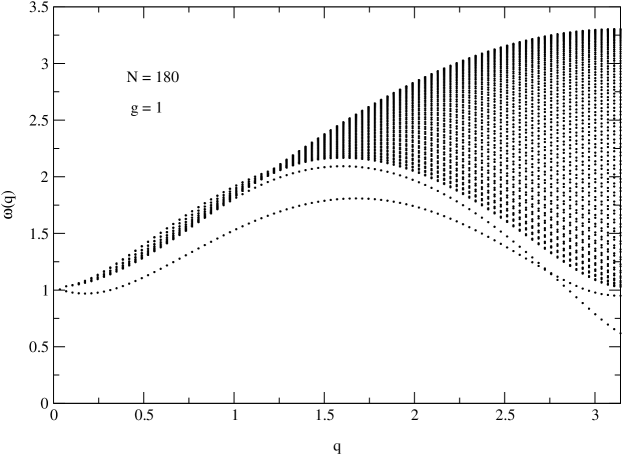
We get the standard RPA from Eqs.(12) in evaluating expectation values with the before elaborated JW-HF groundstate leading to the expressions given in Eq.(13). We show in Fig. 1 for $N=180$ and $g=1$ the RPA eigenvalue spectrum as a function of the momentum transfer $|q|$.

Figure 1: RPA Excitation spectrum for $N=180$ and $g=1$.

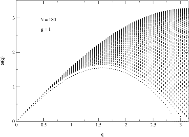
We clearly see that there is a lower branch slightly detached from the more or less dense remainder i.e. the p-h continuum. Actually $N=180$ is already quite close to the thermodynamic limit which we also calculated using the Green function method following closely the work of Todani and Kawasaki [13]. Here we only show the result in Fig. 2.

Figure 2: Excitation spectrum for the infinite chain. The lowest broken line corresponds to the discrete RPA branch. The two upper broken lines limit the RPA p-h continuum. The two full lines limit the continuum in the exact two-spinon case [4] where there is no discrete state.

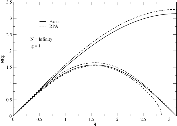
We again see that a lower energy state (lowest broken line) becomes detached from the continuum, the latter being embraced by the two upper broken lines. The continuum was also studied by Todani and Kawasaki [13] but for some reason they did not discuss the low-lying discrete state which is an important and prominent feature. In the thermodynamic limit the dispersion equation of the low-lying branch can be found from (see Ref. [13] Eq.(34))

$$1-f(q,\omega)\Re\left(G^{0}(q,\omega)\right)=0$$ (14)

where $G^{0}(q,\omega)$ is the renormalized particle-hole propagator [13]

$$G^{0}(q,\omega)=\frac{-1}{p\pi\sin(\frac{q}{2})}\frac{1}{2\sqrt{1-x^{2}}}\log\left(\frac{\sqrt{1-x^{2}}+\sin(\frac{q}{2})}{{\sqrt{1-x^{2}}}-\sin(\frac{q}{2})}\right),$$ (15)

and

$$f(q,\omega)=2\cos(q)-2px^{2}$$ (16)

with $\displaystyle x=\frac{\omega+i\eta}{2p\sin(\frac{q}{2})}$ and $\displaystyle p=1+\frac{2}{\pi}$. From Eq. (14) also the lower $\omega_{L}$ and upper $\omega_{U}$ boundaries of the continuum can be obtained

$$\omega_{L}=(1+\frac{2}{\pi})\sin(q)\\ \omega_{U}=2(1+\frac{2}{\pi})\sin(\frac{q}{2}).$$ (17)

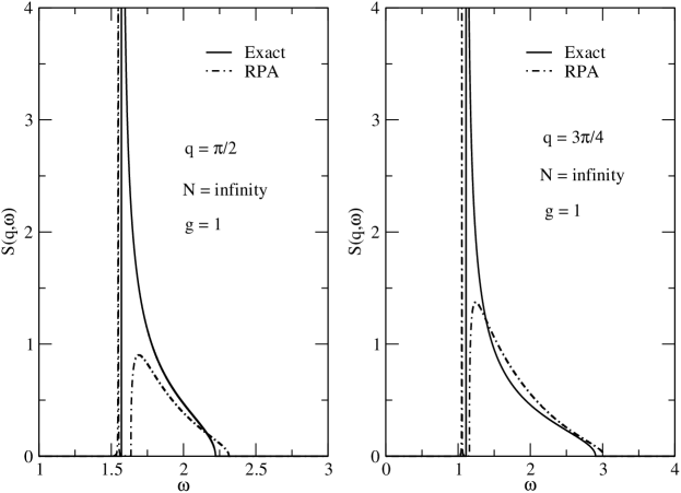
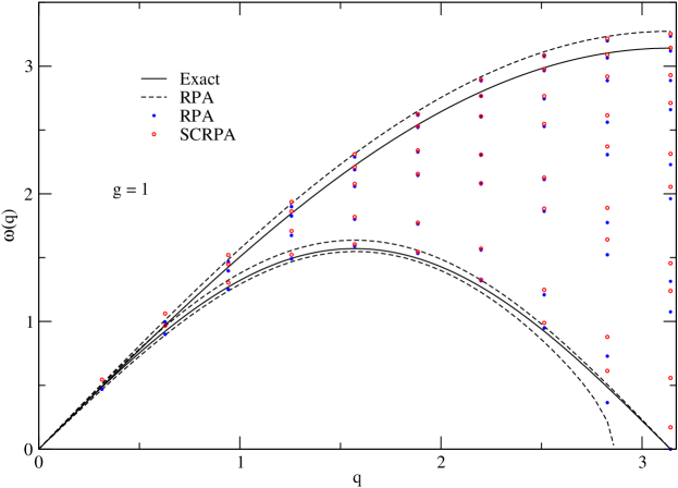
In the exact two-spinon case there is no discrete state and only a continuum limited by the upper $\displaystyle\left(\omega_{U}=\pi\sin(\frac{q}{2})\right)$ and lower $\displaystyle\left(\omega_{L}=\frac{\pi}{2}\sin(q)\right)$ full lines of Fig. 2 exists [14, 4]. The exact two-spinon dynamic structure factor diverges at the lower limit [14, 4]. Nevertheless, globally, the RPA spectrum for the infinite chain resembles the exact solution, even though locally, especially at the lower edge, things go wrong even qualitatively. For instance, the fact that the excitation spectrum exhibits a low lying discrete state detached from the continuum is of course an artefact of the RPA approach. This fact has also very briefly been mentioned in Ref. [15] but no details are given there. We want to point out, however, and this is the main message of the present paper, that the RPA spectrum is already qualitatively quite similar to the exact one as seen in Fig. 3 where we show the structure functions for $\displaystyle q=\frac{\pi}{2}$ and $\displaystyle q=\frac{3\pi}{4}$ corresponding to RPA and exact two-spinon calculation [4]. The detachment of the discrete state is in fact only very mild and we therefore conclude that RPA may be a good starting point for more elaborate theories, even for situations where, a priori, it should not work well as for instance in 1D situation, as considered here.

Let us also mention that in the attractive (ferromagnetic) case quite naturally a discrete state, detached from the continuum, exists, even in the exact solution [16, 15].

Figure 3: Exact two-spinon and RPA dynamic spin structure factor, in the thermodynamic limit, for $\displaystyle q=\frac{\pi}{2}$ and $\displaystyle q=\frac{3\pi}{4}$.

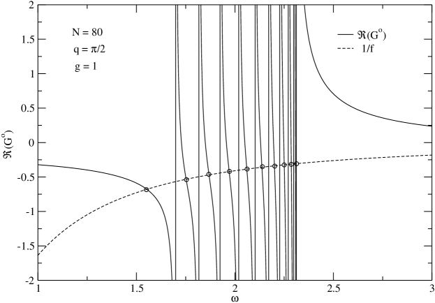
To understand the reason why there exists in RPA a discrete collective state detached from the continuum it is instructive to solve Eq. (14) for the dispersion relations $\omega(q)$ in the case of a finite number of sites. In the discrete case $f(q,\omega)$ actually has a more complicated structure and it only reduces to Eq. (16) in the thermodynamic limit. In order not to overload the figure we choose a somewhat lower value for $N$ than in Fig. 1. We see in Fig. 4 the graphical solution of Eq. (14) for $N=80$. The structure is very similar to other schematic RPA models (see e.g. [11]) with the only difference that the smooth effective interaction is momentum and energy dependent what stems from the fact that here we have a 3-rank separable interaction instead of the usual one rank separability. The collective state gets detached from the more or less unshifted ph-roots precisely because it is situated at the edge of the continuum. One also can make a guess what may happen in the exact case. Due to screening the corresponding effective interaction $f(q,\omega)$ will bend much more strongly at the lower edge of the ph-continuum in such a way that the collective state sticks closely to the last lower vertical asymptote.

Figure 4: Graphical solution of the dispersion relation for $N=80$ and $\displaystyle q=\frac{\pi}{2}$.

The similarity of the RPA structure function with the exact one can also be inferred from studying the corresponding energy weighted sum rules. Let us define

$$\frac{1}{2\pi}\int^{\infty}_{0}\omega S_{zz}(q,\omega)d\omega&=-\frac{2E_{gs}}{3N}(1-\cos(q))\\ {}\frac{1}{2\pi}\int^{\infty}_{0}\omega S^{(2)}_{zz}(q,\omega)d\omega=\frac{C}{\pi}\kappa_{0}(1-\cos(q))\\ {}\frac{1}{2\pi}\int^{\infty}_{0}\omega S^{RPA}_{zz}(q,\omega)d\omega=\frac{1}{\pi}(1-\cos(q)){}$$ (18)

with $C=0.72221...$, $\kappa_{0}=0.9163...$ and $E_{gs}=-N(\log 2-\frac{1}{4})$ being the exact ground-state energy. $S_{zz}(q,\omega)$ is the exact dynamic spin structure factor, $S^{(2)}_{zz}(q,\omega)$ is the exact 2-spinon part of the exact dynamic spin structure factor [4], and $S^{RPA}(q,\omega)$ is the corresponding structure function in the present RPA approach. For $\displaystyle q=\frac{\pi}{2}$, in RPA, the sum rule gives 0.318309 and the contribution to the sum rule from the discrete state is 0.226843 ($71\%$) and from the continuum it is 0.091467 ($29\%$). For $\displaystyle q=\frac{3\pi}{4}$, in RPA, the sum rule gives 0.543389 and the contribution to the sum rule from the discrete state is 0.244919 ($45\%$) and from the continuum it is 0.298470 ($55\%$). From the above we see that the RPA energy weighted sum rule Eq. (LABEL:rsc) within $\sim 50\%$ of the exact two-spinon result Eq. (LABEL:rsb) and within $\sim 8\%$ of the exact result Eq. (LABEL:rsa). This latter result again underlines the semi-quantitative correct behavior of the RPA.

On Figs. 1 and 2 we also see that RPA actually becomes unstable for $q>q_{c}\simeq 0.91\pi$ because the discrete branch touches zero at $q\simeq q_{c}$. An RPA eigenvalue coming down to zero inevitably means that the corresponding HF stability matrix [11, 12]

$${\mathcal{S}}(q)=\pmatrix{A&B\cr B&A}$$ (19)

also has a zero eigenvalue at the critical value $q=q_{c}$ and negative eigenvalues for $q>q_{c}$, clearly indicating that the translationally invariant JW-HF solution is unstable.

The reason why the RPA performs relatively well is probably precisely because we forced the system to remain in the symmetry unbroken, i.e. ’spherical’, phase as it is well known that in 1D no spontaneously symmetry broken phase exists. None the less, we were curious to see what HF and HF-RPA gives in the symmetry broken phase. Not unexpectedly we will find that deformed HF still lowers the energy (see table 1) but HF-RPA leads to an unphysical excitation spectrum. Follow some details of our procedure.

We seek a new HF basis with a stable minimum in introducing new quasiparticle operators which are a superposition of particle (p) and hole (h) operators in the old basis, that is [17]

$$\alpha^{\dagger}_{h+\pi} = u_{h}\psi^{\dagger}_{h+\pi}+v_{h}\psi^{\dagger}_{h}$$ (20)

$$\alpha_{h} = u_{h}\psi^{\dagger}_{h}-v_{h}\psi^{\dagger}_{h+\pi}$$ (21)

with $u^{2}_{h}+v^{2}_{h}=1$. Our ansatz Eq.(21) is motivated by the fact that the mode which becomes unstable occurs at $q=\pi$ and therefore, suggests the order parameter $\langle\psi^{\dagger}_{h+\pi}\psi_{h}\rangle\neq 0$, involving breaking of translational invariance. Following the standard procedure for obtaining the amplitudes $u_{h}$, $v_{h}$ in Eq.(21) we express the HF-energy in the new deformed state

$$\tilde{E}^{HF}_{0} = \frac{gN}{4}+\sum_{h}\left(\epsilon^{o}_{h}+\frac{1}{2}\sum_{h^{\prime}}\bar{v}_{h,h^{\prime},h,h^{\prime}}\right)$$ (22)

$$+ \sum_{h}\bigg{(}\epsilon^{o}_{h+\pi}-\epsilon^{o}_{h}+\sum_{h^{\prime}}\bigg{\{}\bar{v}_{h+\pi,h^{\prime},h+\pi,h^{\prime}}-\bar{v}_{h,h^{\prime},h,h^{\prime}}$$ (23)

$$+ \frac{1}{2}\left(\bar{v}_{h+\pi,h^{\prime}+\pi,h+\pi,h^{\prime}+\pi}+\bar{v}_{h,h^{\prime},h,h^{\prime}}-2\bar{v}_{h+\pi,h^{\prime},h+\pi,h^{\prime}}\right)v^{2}_{h^{\prime}}\bigg{\}}v^{2}_{h}\bigg{)}$$ (24)

$$+ \sum_{hh^{\prime}}\left(\bar{v}_{h+\pi,h^{\prime}+\pi,h,h^{\prime}}+\bar{v}_{h+\pi,h^{\prime},h,h^{\prime}+\pi}\right)u_{h}v_{h}u_{h^{\prime}}v_{h^{\prime}}$$ (25)

and minimize with respect to $u_{h}$, $v_{h}$. We obtain

$$\begin{array}[]{c}u^{2}_{h}\\ v^{2}_{h}\end{array}\bigg{\}}=\frac{1}{2}\left(1\pm\frac{\xi_{h}}{\sqrt{\xi^{2}_{h}+\Delta^{2}_{h}}}\right)$$ (26)

where,

$$\xi_{h} = \epsilon^{o}_{h+\pi}-\epsilon^{o}_{h}+\sum_{h^{\prime}\neq h}\bigg{\{}\bigg{(}\bar{v}_{h+\pi,h^{\prime}+\pi,h+\pi,h^{\prime}+\pi}+\bar{v}_{h,h^{\prime},h,h^{\prime}}$$ (27)

$$- \bar{v}_{h+\pi,h^{\prime},h+\pi,h^{\prime}}-\bar{v}_{h,h^{\prime}+\pi,h,h^{\prime}+\pi}\bigg{)}v^{2}_{h^{\prime}}$$ (28)

$$+ \bar{v}_{h+\pi,h^{\prime},h+\pi,h^{\prime}}-\bar{v}_{h,h^{\prime},h,h^{\prime}}\bigg{\}}$$ (29)

$$\Delta_{h} = -2\sum_{h^{\prime}\neq h}\left(\bar{v}_{h+\pi,h^{\prime}+\pi,h,h^{\prime}}-\bar{v}_{h+\pi,h^{\prime},h^{\prime}+\pi,h}\right)u_{h^{\prime}}v_{h^{\prime}}$$ (30)

With Eq.(26) and Eq.(30) we get the self-consistent ’gap’ equation

$$\Delta_{h} = -2\sum_{h^{\prime}\neq h}\left(\bar{v}_{h+\pi,h^{\prime}+\pi,h,h^{\prime}}-\bar{v}_{h+\pi,h^{\prime},h^{\prime}+\pi,h}\right)\frac{\Delta_{h^{\prime}}}{2\sqrt{\xi^{2}_{h^{\prime}}+\Delta^{2}_{h^{\prime}}}}$$ (31)

$$= \frac{4g}{N}\sum_{h^{\prime}\neq h}\frac{\Delta_{h^{\prime}}}{\sqrt{\xi^{2}_{h^{\prime}}+\Delta^{2}_{h^{\prime}}}}$$ (32)

Solving the gap equation numerically allows us to calculate the new HF energy as a function of $g$. For $N\rightarrow\infty$, Eq. (32) gives a nontrivial solution even for $g\rightarrow 0$.

As a last step we calculate the RPA in the new basis. For this we introduce in analogy to Eq. (11) an RPA excitation operator of the following form

$$Q^{\dagger}_{\nu,q}=\sum_{ph}\tilde{X}^{\nu}_{ph}\alpha^{\dagger}_{p}\alpha^{\dagger}_{h}-\tilde{Y}^{\nu}_{ph}\alpha_{h}\alpha_{p},\quad q=|p-h|$$ (33)

Proceeding in a similar way to what we have done in the spherical basis we can find the amplitudes $\tilde{X},\tilde{Y}$ from corresponding RPA equations. We show the spectrum in Fig. 5. We see that the spectrum now contains a gap corresponding to Eq. (30) and is qualitatively similar to the exact solutions for an anisotropic Heisenberg Hamiltonian ($g\neq 1$) [3].

Figure 5: RPA excitation spectrum in deformed basis in the case of $N=180$.

The fact that the spectrum in Fig. 5 does not resemble much the exact one is not completely surprising, since we know that it is built on qualitatively wrong (symmetry broken) groundstate. However, the relatively good performance of the HF-RPA scheme in the symmetry unbroken phase motivates us to go beyond the standard RPA approach in applying symmetry restoration techniques [11] and Self-Consistent RPA (SCRPA) [5]. The latter has already produced an interesting result for the 1D-AFH model in Ref. [6].

In this work we made a preliminary application of SCRPA to some cases of finite number of sites. Without going into details, let us shortly repeat the principles of SCRPA. It essentially consists in evaluating Eq. (12) not with the HF ground state as in standard RPA but with a ground state containing RPA correlations, as this is the objective proper of RPA. In this exploratory application to the AFH model, we found it most convenient to solve the vacuum condition $Q_{\nu}|0\rangle=0$, mentioned above, pertubatively. Neglecting 3p-3h and higher configurations one obtains [18] :

$$|0\rangle\sim\left(1+\frac{1}{4}\sum_{p_{1},h_{1},p_{2},h_{2}}z_{p_{1},h_{1},p_{2},h_{2}}\psi^{\dagger}_{p_{1}}\psi_{h_{1}}\psi^{\dagger}_{p_{2}}\psi_{h_{2}}\right)|\mbox{HF}\rangle$$ (34)

with

$$z_{p_{1}h_{1},p_{2}h_{2}}=[YX^{-1}]_{p_{1}h_{1},p_{2}h_{2}}$$ (35)

Figure 6: Excitation spectrum $\omega(q)$ as function of the momentum transfer, for $N=6$. Exact results are indicated by black squares, RPA results by blue stars and SCRPA results by red circles.

Figure 7: Excitation spectrum $\omega(q)$ as function of the anisotropy $g$, for $N=6$ and for all momentum transfer. Exact results are indicated by black solid line, RPA results by blue dotted line and SCRPA results by red dashed line. For $g>1$ the RPA results are obtained in the deformed basis.

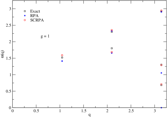
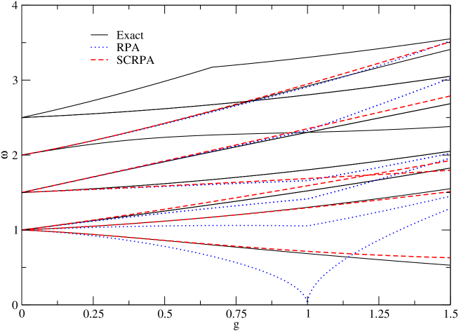
Evaluating Eq. (12) with Eq. (34) yields an RPA matrix which depends in a non-linear way on the amplitudes $X$, $Y$. Solving this non-linear system of equations is numerically not completely trivial and consequently in a first attempt we restricted ourselves to quite small system sizes. In Fig 6 we compare the results from an exact diagonalization for the six sites problem with half filling with the those from SCRPA. We see that there is close agreement and a strong improvement of SCRPA over standard RPA. In Fig. 7 we show the same but as function of the coupling constant g. Again we see the very important improvement of the SCRPA specially around the phase transition point $g=1$. In Fig 8 we also show the SCRPA results for the case of 20-sites at half filling. We see that the lowest branch in SCRPA is strongly lifted up with respect to standard RPA. Though we do not have the exact solution at hand for this case, our results may indicate that in SCRPA no artificial gap is present any longer in the thermodynamic limit. In order to confirm this we have to solve SCRPA in the thermodynamic limit or, at least, approaching it. This shall be an investigation for the near future.

Figure 8: Excitation spectrum $\omega(q)$ as function of the momentum transfer for $N=20$ (also for the thermodynamic limit). For the exact result, in the thermodynamic limit, we present the lower and upper boundary of the spectrum, they are indicated in black color (solid line). For the RPA results, in the thermodynamic limit, we present the collective mode and both boundaries of the continuum states; they are indicated in black color (dashed line). In the discrete case, RPA results are indicated by blue stars and SCRPA results by red circles.

In summary, we evaluated for the first time the full RPA solution for the 1D Anti-Ferromagnetic Heisenberg model in the Jordan-Winger representation. It is shown that one obtains interesting results for spectral functions and sum rules in the symmetry unbroken phase in spite of the fact that a low-lying discrete state gets (slightly) detached from the continuum what is unphysical. The not translationally invariant Hartree-Fock solution still lowers the energy but the corresponding RPA shows, not unexpectedly, a strong artificial gap in the spectrum. The encouraging results of standard RPA motivated us to make a first application of an improved version of RPA, the so-called Self-Consistent RPA (SCRPA) [5] for the time being only for small systems. Strong improvement of the results of SCRPA over standard RPA can be observed. One may speculate that SCRPA cures the artificial gap problem seen in Fig. 3 for the structure function in the thermodynamic limit. The latter is, however, a non trivial numerical problem in SCRPA which we will try to solve in future work.

Acknowledgments

We thank H.-J. Mikeska, J. Villain, T. Ziman for useful discussions and comments. One of us (A.R.) specially acknowledges many useful and elucidating discussions with C. Providência. He also is greatful to the members of theoretical group of the Institut de Physique Nucléaire de Lyon for their hospitality at the beginning of this work. One of us (P.S.) is greatful to D. Foerster for an early collaboration on the present subject. This work has been supported by a grant provided by Fundação para a Ciência e a Tecnologia SFRH/BPD/14831/2003.

References

- [1] W. Heisenberg, Z. Phys. 49, 619 (1928).
- [2] H. Bethe, Z. Phys. 71, 205 (1931).
- [3] H.-J. Mikeska and A. K. Kolezhuk, Lecture Notes in Physics vol.645 (Berlin: Springer), p.1–83 (2004).
- [4] A. H. Bougourzi, M. Couture and M. Kacir, Phys. Rev. B 54, R12669 (1996); M. Karbach, G. Müller, A. H. Bougourzi, A. Fledderjohann, and K.-H. Mütter, Phys. Rev. B 55, 12 510 (1997).
- [5] J.G. Hirsch, A. Mariano, J. Dukelsky, P. Schuck, Ann. Phys. 296, 187 (2002); A. Rabhi, R. Bennaceur, G. Chanfray, and P. Schuck, Phys. Rev. C 66, 064315 (2002); A. Storozhenko, P. Schuck, J. Dukelsky, G. Röpke, A. Vdovin, Ann. Phys. 307, 308 (2003); M. Jemai, P. Schuck, J. Dukelsky and R. Bennaceur, Phys. Rev. B 71, 085115 (2005).
- [6] P. Krüger and P. Schuck, EuroPhys. Lett. 72, 395 (1994).
- [7] M. Takahashi, Phys. Rev. B 40, 2494 (1989).
- [8] P. Jordan and E. Wigner, Z. Phys. 47, 631 (1928).
- [9] S. Rodriguez, Phys. Rev. 116, 1474–1477 (1959); E. Lieb, T. Schultz, and D. Maltis, Ann. Phys. (N.Y.) 16, 407 (1961); L. N. Bulaevski, Sov. Phys. JETP 16, 685 (1963).
- [10] D.J. Rowe, Phys. Rev. 175, 1283 (1968); Rev. Mod. Phys. 40, 153 (1968).
- [11] P. Ring and P. Schuck, The Nuclear Many-Body Problem, Springer, Berlin (1980)
- [12] D. J. Thouless, Nucl. Phys. 22, 78 (1961).
- [13] T. Todani and K. Kawasaki, Prog. Theor. Phys. 50, 1216 (1973).
- [14] G. Müller, H. Thomas, H. Beck, and J. C. Bonner, Phys. Rev. B 24, 1429 (1981).
- [15] T. Schneider, E. Stoll, and U. Glaus, Phys. Rev. B 26, 1321 (1982).
- [16] H. Beck and G. Müller, Solid State Commun. 43, 399 (1982).
- [17] A. Auerbach, Interacting Electrons and Quantum Magnetism, Springer-Verlag, New York (1994).
- [18] D. S. Delion, P. Schuck and J. Dukelsky, Phys.Rev. C 72, 064305 (2005); D. Gambacurta, M. Grasso, F. Catara, and M. Sambataro, Phys. Rev. C 73, 024319 (2006).