Model C critical dynamics of disordered magnets

Abstract

The critical dynamics of model C in the presence of disorder is considered. It is known that in the asymptotics a conserved secondary density decouples from the nonconserved order parameter for disordered systems. However couplings between order parameter and secondary density cause considerable effects on non-asymptotic critical properties. Here, a general procedure for a renormalization group treatment is proposed. Already the one-loop approximation gives a qualitatively correct picture of the diluted model C dynamical criticality. A more quantitative description is achieved using two-loop approximation. In order to get reliable results resummation technique has to be applied.

, ,

1 Introduction

The relevance of weak structural disorder for the critical behaviour of pure magnetic systems has been in the focus of attention of researchers since a long time [1]. Depending on the structure of a magnet disorder can enter as random fields, random anisotropies, random bond or site dilution. Our special interest here is in diluted systems. Concerning the statics of such systems one of the main insights comes from the Harris criterion [2] stating that the static asymptotic critical behaviour remains unchanged, if the specific heat of the pure system does not diverge [3]. Since the borderline value $n_{c}$ between a diverging and nondiverging specific heat in space dimension $d=3$ lies between order parameter (OP) dimension $n=1$ (Ising model) and $n=2$ (XY model) [4] only diluted Ising systems show a new critical behaviour, which is characterized by a non-diverging specific heat [1].

Systems with the same static critical behaviour may have different dynamic critical properties. In the vicinity of a critical point slow processes play an important role, therefore in critical dynamics the main objects are the slow modes. Apart from the order parameter these are the conserved quantities, which coupled to the OP. The simplest dynamical model - model C [5] - includes these couplings only statically. For such a case the Harris criterion also has consequences. It leads to the conclusion that the coupling of conserved quantities to the OP in disordered systems is of no relevance [6, 7, 8]. The argumentation of this statement is based on the fact [5, 9, 10] that coupling to a conserved density for the relaxational model is relevant only if the specific heat diverges. Diluted models always have nondiverging specific heat and therefore their coupling beetwen a conserved density and OP is irrelevant. As a consequence most of the studies of critical dynamics considered only relaxational dynamics of diluted Ising systems [11, 12, 13, 14].

However the conclusion concerning the irrelevance of the conserved density is made only for the asymptotic properties of the model. Meanwhile it became clear that in diluted magnets most of the experiments and simulations are in the nonasymptotic region [1, 15, 16, 17, 18, 19]. Within the standard tool of investigation of critical phenomena, namely the field-theoretical renormalization group (RG), the nonasymptotic critical behaviour is described by the flow of the model parameters (static and dynamic) leading to effective critical behaviour rather than to the asymptotic one characterized by power laws with universal exponents determined by the fixed point properties of the parameters.

Thus we consider the dynamics of a diluted magnetic system where the OP relaxes with a relaxation rate $\Gamma$ and the second conserved density shows diffusive behaviour with a diffusion rate $\lambda$. The ratio of the time scales $w=\Gamma/\lambda$ is the dynamic parameter of model C and takes on different fixed point values depending on the dimension $n$ of the OP and spatial dimension $d$. Only recently the correct field theoretic RG functions of model C have been calculated [9, 10]. It turned out that model C itself has a very slow transient at least for the cases $n=1,2$ in two-loop order.

Another artifact present in the RG analysis of diluted magnets within one loop order is the degeneracy of the static $\beta$-functions for $n=1$. As it is well established now it leads to a $\sqrt{4-d}$ rather than a $4-d$-expansion [20, 21]. This makes a two-loop treatment inevitable. Moreover the borderline where the specific heat exponent $\alpha$ changes in two-loop order is shifted from $n=4$ to below $n=2$.

Thus two-loop calculations are necessary (i) to specify the shift of the stability regions and (ii) to calculate quantitative values of the effective exponents.

All the above arguments serve as a reason to consider the disordered model C critical dynamics by the field-theoretical RG approach within two-loop approximation. Being more elaborated technically this approximation should lead to reliable numerical results which as previous experience shows should not be changed essentially by further increase of the perturbation theory order. Some of our results are briefly summarized in Ref. [30], and here we give a more thorough derivation of the dynamic RG function and analyze the diluted model C effective critical dynamics.

The set-up of the paper is the following: in the next Section we define the dynamical model for disordered magnets, its renormalization and general relations for the field theoretic functions. Results in one-loop order are collected in Section 3. Two-loop results are presented in Section 4. Conclusions are given in Section 5.

2 Model and renormalization

2.1 Model equations

The object of our analysis consists in a dynamical model for quenched disordered magnets, namely model C in the classification of Ref.[22]. Model C describes the dynamics of a nonconserved OP $\vec{\varphi}_{0}$ which is coupled to a conserved density $m_{0}$ (in most cases the energy density). The secondary density has to be taken into account since it is also a slow density showing critical slowing down near the phase transition. The OP is assumed to be an $n$-component vector, while the density $m_{0}$ is a scalar quantity. The structure of the equations [22, 5] of motion is not changed by the presence of disorder. They read:

$$\frac{\partial{\varphi}_{i,0}}{\partial t} = -\mathring{\Gamma}\frac{\partial{\mathcal{H}}}{\partial{\varphi}_{i,0}}+{\theta}_{{\varphi}_{i}}\qquad i=1\ldots n,$$ (1)

$$\frac{\partial{m}_{0}}{\partial t} = \mathring{\lambda}_{m}\nabla^{2}\frac{\partial{\mathcal{H}}}{\partial{m}_{0}}+{\theta_{{m}}}.$$ (2)

The OP relaxes to equilibrium with the relaxation rate $\mathring{\Gamma}$ and the conserved density $m_{0}$ diffuses with the diffusion rate $\mathring{\lambda}_{m}$. The stochastic forces in (1), (2) satisfy the Einstein relations:

$$<{\theta}_{\varphi_{i}}(x,t){\theta}_{\varphi_{j}}(x^{\prime},t^{\prime})> = 2\mathring{\Gamma}\delta(x-x^{\prime})\delta(t-t^{\prime})\delta_{ij},$$ (3)

$$<{\theta}_{m}(x,t){\theta}_{{m}}(x^{\prime},t^{\prime})> = -2\mathring{\lambda}_{{m}}\nabla^{2}\delta(x-x^{\prime})\delta(t-t^{\prime})\delta_{ij}.$$ (4)

In order to define model C in the presence of structural disorder we write the static functional $\mathcal{H}$ describing the behaviour of a disordered magnetic system in equilibrium:

$${\mathcal{H}} = \int d^{d}x\Big{\{}\frac{1}{2}\mathring{\tilde{r}}|\vec{\varphi}_{0}|^{2}+V(x)|\vec{\varphi}_{0}|^{2}+\frac{1}{2}\sum_{i=1}^{n}(\nabla\varphi_{i,0})^{2}+$$ (5)

$$\frac{\mathring{\tilde{u}}}{4!}|\vec{\varphi}_{0}|^{4}+\frac{1}{2}a_{{m}}{{m_{0}}}^{2}+\frac{1}{2}\mathring{\gamma}_{{m}}{{m_{0}}}|\vec{\varphi}_{0}|^{2}-\mathring{h}_{{m}}{{m_{0}}}\Big{\}},$$

where $V(x)$ is an impurity potential which introduces disorder to the system, and $d$ is the spatial dimension. The functional (5) contains a coupling $\mathring{\gamma}_{m}$ to the secondary density which can be integrated out. Thus static critical properties described by the functional (5) are equivalent to those of a Ginzburg-Landau-Wilson (GLW) functional:

$${\mathcal{H}}=\int d^{d}x\Big{\{}\frac{1}{2}\mathring{r}|\vec{\varphi}_{0}|^{2}{+}V(x)|\vec{\varphi}_{0}|^{2}{+}\frac{1}{2}\sum_{i{=}1}^{n}(\nabla\varphi_{i,0})^{2}{+}\frac{\mathring{u}}{4!}|\vec{\varphi}_{0}|^{4}\Big{\}}.$$ (6)

The parameters $\mathring{r}$ and $\mathring{u}$ are related to $\mathring{\tilde{r}}$, $\mathring{\tilde{u}}$, $a_{m}$, $\mathring{\gamma}_{m}$ and $\mathring{h}_{m}$ by

$$\mathring{r} = \mathring{\tilde{r}}+\frac{\mathring{\gamma}_{{m}}\mathring{h}_{{m}}}{a_{m}},\qquad\mathring{u}=\mathring{\tilde{u}}-3\frac{\mathring{\gamma}_{{m}}^{2}}{a_{m}},$$ (7)

$\mathring{r}$ is proportional to the temperature distance from the mean field critical temperature, $\mathring{u}$ is positive.

The properties of the random potential $V(x)$ are governed by a Gaussian distribution

$${\mathcal{P}}_{V}={\mathcal{N}}_{V}\exp\left(-\frac{\int d^{d}x{V(x)^{2}}}{8\mathring{\Delta}}\right).$$ (8)

with positive width $\mathring{\Delta}$, which is proportional to the concentration of non-magnetic impurities.

For investigation of statics in the further procedure one has to take into account that the disorder is quenched. Averaging the free energy of a disordered system over the distribution (8) with application of the replica trick [23] one ends up with an effective static functional containing new terms determined by disorder [21]. Then critical properties are studied on the basis of long-distance properties of the effective functional.

The procedure for the critical dynamics may be different. We will treat the critical dynamics of the disordered models within the field theoretical RG method based on the Bausch-Janssen-Wagner approach [24], where the appropriate Lagrangians of the models are studied. Therefore we have to obtain the Lagrangian for our model on the basis of the model equations (1)-(5). Then after averaging over the random potential (8) we get new terms determined by the disorder in the Lagrangian. In this case it is not necessary to apply the replica method [25]. Results can be written in the form (for details see A) ${\mathcal{L}}={\mathcal{L}}_{0}+{\mathcal{L}}_{int}$ with the Gaussian (unperturbed) part:

$${\mathcal{L}}_{0}=\int d^{d}xdt\Bigg{\{}{-}\mathring{\Gamma}\sum_{i=1}^{n}{\tilde{\varphi}_{0,i}}{\tilde{\varphi}_{0,i}}{+}\sum_{i=1}^{n}{\tilde{\varphi}_{0,i}}\left({\frac{\partial}{\partial t}}{+}\mathring{\Gamma}(\mathring{r}{-}\nabla^{2})\right)\varphi_{0,i}$$

$$+\mathring{\lambda}_{m}\tilde{m}_{0}\nabla^{2}\tilde{m}_{0}+\tilde{m}_{0}\left({\frac{\partial}{\partial t}}-a_{m}\mathring{\lambda}_{m}\nabla^{2}\right)m_{0}\Bigg{\}},$$ (9)

and an interaction part:

$${\mathcal{L}}_{int}{=}\int d^{d}xdt\sum_{i}\Bigg{\{}\frac{1}{3!}\mathring{\Gamma}\mathring{u}\tilde{\varphi}_{0,i}{\varphi}_{0,i}\sum_{j}{\varphi}_{0,j}{\varphi}_{0,j}{-}\int\!dt^{\prime}\!\sum_{j}\!2\mathring{\Gamma}^{2}{\mathring{\Delta}}\tilde{\varphi}_{0,i}(x,t){\varphi}_{0,i}(x,t)$$

$$\times\tilde{\varphi}_{0,j}(x,t^{\prime}){\varphi}_{0,j}(x,t^{\prime})+\mathring{\Gamma}\mathring{\gamma}_{m}m_{0}\tilde{\varphi}_{0,i}{\varphi}_{0,i}{-}\frac{1}{2}\mathring{\lambda}_{m}\mathring{\gamma}_{m}\tilde{m}_{0}\nabla^{2}{\varphi}_{0,i}{\varphi}_{0,i}\Bigg{\}}\,,$$ (10)

with new auxiliary response fields $\tilde{\varphi}_{0,i}$. The ratio $\mathring{u}/\mathring{\Delta}$ determines the degree of disorder in the system.

Investigating the long-distance and long-time properties of the theory with the effective Lagrangian ${\mathcal{L}}$ we apply Feynman diagram techniques in order to get dynamical vertex functions. Details of the calculation of the dynamic vertex function $\mathring{\Gamma}_{\tilde{\varphi},\varphi}$ are given in A. The renormalization of vertex functions leads to the RG functions, describing the critical dynamics of our model. We use the minimal subtraction scheme with dimensional regularization to calculate these functions. General relations are considered in the next subsections. The details concerning the renormalization procedure are given in B.

2.2 RG functions

From the renormalizing factors introduced in B we define the $\zeta$-functions which describe the critical behaviour of our model

$$\zeta_{a_{i}}(\{\alpha_{i}\}) = -\frac{d\ln Z_{a_{i}}}{d\ln\mu}\,,$$ (11)

here $\{\alpha_{i}\}=\{u,\Delta,\gamma,\Gamma,\lambda\}$ represents the set of renormalized parameters for the disordered model C and $\mu$ is the scale. The notation $a_{i}$ denotes any density ($\varphi$, $\tilde{\varphi}$, $m$, $\tilde{m}$) or any model parameter $\alpha_{i}$.

A special case is the additive renormalization $A_{\varphi^{2}}$ of the specific heat in the GLW-model. It leads to an additional RG function

$$B_{\varphi^{2}}(u,\Delta)=\mu^{\varepsilon}Z^{2}_{\varphi^{2}}\mu\frac{d}{d\mu}\left(Z^{-2}_{\varphi^{2}}\mu^{-\varepsilon}A_{\varphi^{2}}\right)\,,$$ (12)

which appears in the static and dynamic $\zeta$-functions.

Since in statics the secondary field can be integrated out one finds relations to the static $Z$-factors appearing in model A (see B). The relations (69) and (67) lead then to

$$\zeta_{\gamma}(u,\Delta,\gamma)=2\zeta_{m}(u,\Delta,\gamma)+\zeta_{\varphi}(u,\Delta)+\zeta_{\varphi^{2}}(u,\Delta),$$ (13)

and

$$\zeta_{m}(u,\Delta,\gamma)=\frac{1}{2}\gamma^{2}B_{\varphi^{2}}(u,\Delta).$$ (14)

Eliminating $\zeta_{m}$ by inserting Eq. (14) into Eq. (13) one gets:

$$\zeta_{\gamma}(u,\Delta,\gamma)=\gamma^{2}B_{\varphi^{2}}(u,\Delta)+\zeta_{\varphi}(u,\Delta)+\zeta_{\varphi^{2}}(u,\Delta).$$ (15)

The $\zeta$-functions for the kinetic coefficients $\Gamma$ and $\lambda$, which are obtained by substituting relations (65) and (73) into the definition (11), read

$$\zeta_{\Gamma}(\{u,\Delta,\gamma,w\}){=}{-}\frac{1}{2}\zeta_{\tilde{\varphi}}(\{u,\Delta,\gamma,w\}){+}\frac{1}{2}\zeta_{\varphi}(u,\Delta),$$ (16)

$$\zeta_{\lambda}(u,\gamma){=}\gamma^{2}B_{\varphi^{2}}(u,\Delta).$$ (17)

The last relation is obtained taking into account Eq. (14).

In order to investigate the dynamical fixed points of model C it is convenient to introduce the time scale ratio $w={\Gamma}/{\lambda}$. The corresponding $\zeta$-function for this dynamical parameter using the relations (16) and (17) reads:

$$\zeta_{w}(u,\Delta,\gamma,w)=\frac{1}{2}\zeta_{\varphi}(u,\Delta)-\frac{1}{2}\zeta_{\tilde{\varphi}}(u,\Delta,\gamma,w)-\gamma^{2}B_{\varphi^{2}}(u,\Delta)\,.$$ (18)

The static critical properties of our model are described by the flow equations:

$$l\frac{du}{dl}=\beta_{u}(u,\Delta),\quad l\frac{d\Delta}{dl}=\beta_{\Delta}(u,\Delta),\quad l\frac{d\gamma}{dl}=\beta_{\gamma}(u,\Delta,\gamma),$$ (19)

with the flow parameter $\ell$ and $\beta$-functions generally defined as

$$\beta_{\alpha_{i}}(\{\alpha_{i}\})=\alpha_{i}[-c_{i}+\zeta_{\alpha_{i}}(\{\alpha_{i}\})],$$ (20)

where $c_{i}$ are the engineering dimensions of the corresponding parameters $\alpha_{i}$. Following Eq. (20) we can rewrite the static $\beta$-functions:

$$\beta_{u}({u,\Delta})=u\left(-{\varepsilon}-2\zeta_{\varphi}(u,\Delta)+\zeta_{u}(u,\Delta)\right),$$ (21)

$$\beta_{\Delta}({u,\Delta})=\Delta\left(-{\varepsilon}-2\zeta_{\varphi}(u,\Delta)+\zeta_{\Delta}(u,\Delta)\right),$$ (22)

$$\beta_{\gamma}({u,\Delta,\gamma})=\gamma\Bigg{(}-\frac{\varepsilon}{2}-\zeta_{\varphi}(u,\Delta)-\zeta_{m}(u,\Delta,\gamma)+\zeta_{\gamma}(u,\Delta,\gamma)\Bigg{)}.$$ (23)

Note that the flow equations for $u$ and $\Delta$ are independent from those for the other model parameters. They are the same as for the diluted $n$-vector model.

The dynamical critical properties are determined by the flow equation for the time scale ratio $w$, which reads

$$l\frac{dw}{dl} = \beta_{w}(u,\Delta,\gamma,w),$$ (24)

where the $\beta$-function for $w$, according to Eq. (20), is defined as

$$\beta_{w}({u,\Delta,\gamma,w})=w\zeta_{w}(u,\Delta,\gamma,w),$$ (25)

since $\Gamma$, $\lambda$ and their ratio $w$ are dimensionless parameters.

Using the relations between $\zeta$-functions for $\beta_{\gamma}$ and $\beta_{w}$ one obtains:

$$\beta_{\gamma}({u,\Delta,\gamma}) = \gamma\left(-\frac{\varepsilon}{2}+\zeta_{\varphi^{2}}(u,\Delta)+\frac{1}{2}{\gamma^{2}}B_{\varphi^{2}}(u,\Delta)\right)$$ (26)

$$= \gamma\left(-\frac{{\cal A}(u,\Delta)}{2}+\frac{1}{2}{\gamma^{2}}B_{\varphi^{2}}(u,\Delta)\right).$$

$$\beta_{w}({u,\Delta,\gamma,w})=w\Bigg{(}\frac{1}{2}\zeta_{\varphi}(u,\Delta)-\frac{1}{2}\zeta_{\tilde{\varphi}}(u,\Delta,\gamma,w) - \gamma^{2}B_{\varphi^{2}}(u,\Delta)\Bigg{)}.$$ (27)

where ${\cal A}=\varepsilon-2\zeta_{\varphi^{2}}(u,\Delta)$ equals the ratio of coupling dependent functions of the critical exponents of the heat capacity $\alpha(u,\Delta)$ and the correlation length $\nu(u,\Delta)$.

2.3 Asymptotic properties

The common zeroes of the $\beta$-functions (21),(22),(26),(27) define the fixed point (FP) values: $\{\alpha^{*}\}=\{u^{*},\Delta^{*},\gamma^{*},w^{*}\}$. The zeroes of the functions $\beta_{u}$ and $\beta_{\Delta}$ can be obtained independent from the other $\beta$-functions. For each pair of FPs $\{u^{*},\Delta^{*}\}$ one obtains two values of $\gamma^{*}$ from $\beta_{\gamma}$:

$${\gamma^{*}}^{2}{=}0\quad{\rm and}\quad{\gamma^{*}}^{2}{=}\frac{{\cal A}(u^{*},\Delta^{*})}{B_{\varphi^{2}}(u^{*},\Delta^{*})}{=}\frac{\alpha}{\nu B_{\varphi^{2}}(u^{*},\Delta^{*})},$$ (28)

where $\alpha$ and $\nu$ are static heat capacity and correlation length critical exponent calculated at the corresponding FP $\{u^{*},\Delta^{*}\}$. Then the results for the static FPs are inserted into $\beta_{w}$ in order to find the corresponding values of $w^{*}$.

The relevant FP corresponding to a critical point of the system has to be (i) accessible from the physical initial conditions and (ii) stable. The stability of a FP is defined by the eigenvalues $\omega_{i}$ of the matrix ${\partial\beta_{j}}/{\partial\alpha_{i}}$. If the real parts of all $\omega_{i}$ calculated at some FP $\{\alpha^{*}\}$ are positive then the FP $\{\alpha^{*}\}$ is stable and the flow of the system of differential equations (19) and (24) is attracted to this FP in the limit $\ell\to 0$.

From the structure of the stability matrix we conclude, that the stability of any FP with respect to the parameters $\gamma$ and $w$ is determined solely by the derivatives of the corresponding $\beta$-functions:

$$\omega_{\gamma}=\frac{\partial\beta_{\gamma}}{\partial{\gamma}},\qquad\omega_{w}=\frac{\partial\beta_{w}}{\partial{w}}.$$ (29)

Moreover using (26) we can write:

$$\omega_{\gamma}=-\frac{{\cal A}(u,\Delta)}{2}+\frac{3}{2}\gamma^{2}B_{\varphi^{2}}(u,\Delta)\,,$$ (30)

which at the FP ${\alpha^{*}_{i}}$ leads to:

$$\left.\omega_{\gamma}\right|_{{\alpha_{i}}={\alpha^{*}_{i}}} = -\frac{\alpha}{2\nu}\qquad{\rm for}\qquad{\gamma^{*}}^{2}=0\,,$$ (31)

$$\left.\omega_{\gamma}\right|_{{\alpha_{i}}={\alpha^{*}_{i}}} = \frac{\alpha}{\nu}\qquad{\rm for}\qquad{\gamma^{*}}^{2}\neq 0\,.$$ (32)

Therefore stability with respect to the parameter $\gamma$ is determined by the sign of $\alpha$. For a system with non-diverging heat capacity ($\alpha<0$) at the critical point, $\gamma^{*}=0$ is the stable FP. Diluted magnets we consider here always have $\alpha<0$ [1]. This leads to the conclusion that in the asymptotic region the secondary density decouples from the OP [6, 7, 8].

The critical exponents are defined by the FP values of the $\zeta$-functions. For instance, the asymptotic dynamical critical exponent $z$ (at the stable FP) is expressed in the following way:

$$z=2+\zeta_{\Gamma}(u^{*},\Delta^{*},\gamma^{*},w^{*}),$$ (33)

while its effective counterpart in the non-asymptotic region is defined by the solution of flow equations (19) and (24) as

$$z_{\rm eff}=2+\zeta_{\Gamma}(u(\ell),\Delta(\ell),\gamma(\ell),w(\ell)).$$ (34)

In the limit $\ell\to 0$ the effective exponents reach their asymptotic values.

3 Results in one-loop order

Although the one-loop order results have the drawbacks mentioned in the introduction one gets a qualitatively correct picture of the effects of disorder on the dynamics. Therefore we discuss this case in more detail.

We are interested in the dynamical properties of disordered model C within the first nontrivial order of expansion in renormalized couplings, that is the one-loop order. The static functions $\beta_{u}$ and $\beta_{\Delta}$ for disordered systems are known in higher loop approximation [26]. However taking the same order for statics as for dynamics, we restrict the expressions for $\beta_{u}$ and $\beta_{\Delta}$ to the one-loop approximation:

$$\beta_{1u} = u\left(-{\varepsilon}+\frac{n+8}{6}u-{24\Delta}\right),$$ (35)

$$\beta_{1\Delta} = \Delta\left(-{\varepsilon}-{16\Delta}+\frac{n+2}{3}u\right).$$ (36)

Note that the region of physical relevance of the couplings $u,\Delta$ for diluted magnets is restricted by $u\geq 0$, $\Delta\geq 0$. The other $\beta_{\gamma}$ is obtained using the static one-loop $\zeta$-function:

$$\beta_{1\gamma} = \gamma\left(-\frac{\varepsilon}{2}-{4\Delta}+\frac{n+2}{6}u+\frac{1}{2}\frac{\gamma^{2}n}{2}\right),$$ (37)

For obtaining the dynamic function $\beta_{w}$, we should first calculate the renormalizing factor $Z_{\tilde{\varphi}}$. From the one-loop part of $Z_{\tilde{\varphi}}$ (see A) following formula (11) we can obtain the $\zeta_{\tilde{\varphi}}$-function. Using obtained result together with one-loop static $\zeta$-functions we get $\beta_{w}$ in the following form:

$$\beta_{w} = w\left({4\Delta}+\gamma^{2}\frac{w}{1+w}-\frac{\gamma^{2}n}{2}\right).$$ (38)

Table 1: One-loop FPs of model C with disorder and their stability for $\varepsilon=4-d>0$. Note that ${\gamma^{*}}^{2}$ has to be positive for the existence of a real FP. .

• FP	$u^{*}$	$\Delta^{*}$	${\gamma^{*}}^{2}$	$\rho^{*}$	stability
  G	0	0	0	$0\leq\rho^{*}\leq 1$	unstable
  				0
  G′			$\frac{2}{n}\varepsilon$	$n/2$	unstable
  				1
  P	$\frac{6\varepsilon}{n+8}$	0	0	$0\leq\rho^{*}\leq 1$	marginal for $n>4$
  				0
  P′			$\frac{2}{n}\frac{(4-n)\varepsilon}{n+8}$	$n/2$	unstable
  				1
  U	0	$-\frac{3\varepsilon}{4}$	0	0	unstable
  				1
  				0	unstable
  U′			$\frac{\varepsilon}{n}$	$3n/4$	stable for $n<4/3$
  				1	stable for $n>4/3$
  M	$\frac{3\varepsilon}{2(n-1)}$	$\frac{(4-n)\varepsilon}{32(n-1)}$	0	0	stable for $1<n<4$
  				1	unstable
  				0	unstable
  M′			$\frac{2}{n}\frac{n-4}{4(n-1)}\varepsilon$	$3n/4$	ustable
  				1	unstable

Setting the right hand side of Eqs. (35)-(38) equal to zero we obtain the system of equations for the FPs. The structure of the functions $\beta_{u}$ and $\beta_{\Delta}$ leads to the existence of four FPs: the Gaussian FP G $\{u^{*}=0,\Delta^{*}=0\}$ , the ’polymer’ FP U $\{u^{*}=0,\Delta^{*}\neq 0\}$, the FP of the pure system P $\{u^{*}\neq 0,\Delta^{*}=0\}$ and the mixed FP M $\{u^{*}\neq 0,\Delta^{*}\neq 0\}$. Depending on the FP values $u^{*}$ and $\Delta^{*}$ values for the genuine model C parameters can be found. As it was already mentioned two values ${\gamma^{*}}^{2}=0$ or ${\gamma^{*}}^{2}\neq 0$ correspond to each FP, this doubles the number of fixed points, see Table 1. We note that the FPs with nonzero ${\gamma^{*}}^{2}$ are indicated by a prime ^′. We do not consider further the FPs U and U^′ since these FPs lie outside the physical region of positive values of $\Delta$.

Among the rest of the FPs only one is stable depending on the OP dimension $n$. For $n>4$ FP P is stable while for $1<n<4$ FP M is stable. Thus the one-loop value of marginal dimension $n_{c}(\varepsilon)=4$ defines the borderline where $\alpha=0$. In higher-loop order the FPs picture is not changed apart from a change of the borderline function $n_{c}(\varepsilon)$. Estimates obtained on the basis of six-loop order calculations [4] give definitely $n_{c}<2$ at $d=3$.

In order to discuss the dynamical FPs it turns out to be useful to introduce the parameter $\rho=w/(1+w)$ which maps $w$ and its FPs on a finite region of the parameter space. Then instead of the flow equation (24) the flow equation for $\rho$ arises:

$$l\frac{d\rho}{dl}=\beta_{\rho}(u,\gamma,\rho),$$ (39)

where according to (25)

$$\beta_{\rho}(u,\gamma,\rho)=\rho(\rho-1)\zeta_{w}(u,\gamma,\rho)\,.$$ (40)

Setting the right side of (40) to zero and using the FP values from Table 1 the values of $\rho^{*}$ can be found. They are shown in Table 1 as well.

Each non-zero solution of ${\gamma^{*}}^{2}$ leads according to (39) to three dynamical FPs: either with $\rho^{*}=0$ (i.e. $w^{*}{=}0$), $\rho^{*}{=}1$ (i.e. $w^{*}{=}\infty$) or $0<\rho^{*}<1$ correspondingly. For the FP which corresponds to ${\gamma^{*}}^{2}=0$ the situation is the following. For the FP M only two dynamical FPs with $\rho^{*}=0$ and $\rho^{*}=1$ exist, while for the FPs P and G any value of $\rho^{*}$ between 0 and 1 is allowed. Checking the stability of these FPs we see that for $1<n<4$ only FP M with $\rho^{*}=0$ is stable. The corresponding one-loop asymptotic value of the dynamical critical exponent in this case coincides with the one-loop result for the pure relaxational model (model A) with disorder: $z=2+\frac{(4-n)\varepsilon}{8(n-1)}$ [11, 7]. For $n>4$ FP P is marginal, all other FPs are unstable. Formally flow starting from the initial values with $\rho_{i}$ ends up at some FP P with $\rho^{*}(\rho_{i})$ depending on the initial value $\rho_{i}$. Thus one gets a whole line of FPs at $u^{*}\not=0$, $\Delta^{*}=\gamma^{*}=0$. In this case the one-loop result for $z$ coincides with the conventional theory value $z=2$. Since in one-loop approximation $n_{c}(\varepsilon)=4$ the FPs M and P determine the critical behaviour of the disordered model C for $n<4$ and $n>4$ respectively.

4 Two-loop results

Static RG functions are already known in high-order approximations within different renormalization schemes (for references see e. g. Ref [1]). Two-loop expressions for functions $\beta_{u}$, $\beta_{\Delta}$, $\beta_{\gamma}$ within the minimal subtraction scheme can be obtained in the replica limit from results of Ref. [31] and they read:

$$\beta_{u}=\beta_{1u}+u\Big{(}-\frac{3m+14}{12}u^{2}+\frac{22m+116}{3}u\Delta-328\Delta^{2}\Big{)},$$ (41)

$$\beta_{\Delta}=\beta_{1\Delta}+\Delta\Big{(}-5\frac{m+2}{36}u^{2}+22\frac{m+2}{3}u\Delta-168\Delta^{2}\Big{)},$$ (42)

$$\beta_{\gamma}=\beta_{1\gamma}+\gamma\Big{(}-\frac{5(m+2)}{72}u^{2}+\frac{5(m+2)}{3}u\Delta-20\Delta^{2}\Big{)}.$$ (43)

The dynamical function $\beta_{\rho}$ is given by formulas (18) and (40), where functions $\zeta_{\tilde{\varphi}}$ and $\zeta_{\varphi}$ are needed also for the calculation of the dynamical critical exponent $z$, $B_{\varphi^{2}}$ is the same as in one-loop approximation. $\zeta_{\varphi}$ can be obtained in the replica limit from results of Ref. [31]:

$$\zeta_{\varphi}=-\frac{m+2}{72}u^{2}+\frac{m+2}{3}u\Delta-4\Delta^{2}.$$ (44)

For the calculation of $\zeta_{\tilde{\varphi}}$ we use the RG scheme described in detail in Appendices A and B. We obtain $\zeta_{\tilde{\varphi}}$ from the two-loop value of $Z_{\tilde{\varphi}}$ (B) , according to the definition (11) it reads:

$$\zeta_{\tilde{\varphi}}=-8{\Delta}+3\frac{n+2}{3}u\Delta-44\Delta^{2}-\frac{n+2}{6}{u}^{2}\left(\ln\frac{4}{3}-\frac{1}{12}\right)-2{\gamma^{2}}\frac{w}{1+w}$$

$$+\Bigg{[}\frac{n+2}{3}u\left(1-3\ln\frac{4}{3}\right)$$

$$+{\gamma^{2}}\frac{w}{1{+}w}\Bigg{(}\frac{n}{2}-\frac{w}{1{+}w}-\frac{3(n{+}2)}{2}\ln\frac{4}{3}-\frac{1{+}2w}{1{+}w}\ln\frac{(1{+}w)^{2}}{1{+}2w}\Bigg{)}\Bigg{]}{\gamma^{2}}\frac{w}{1{+}w}$$

$$-12\Delta{\gamma^{2}}\frac{w}{1{+}w}+4{\Delta}{\gamma^{2}}\frac{w}{1{+}w}\Bigg{[}{w}\ln\frac{w}{1{+}w}-{3}\ln(1+w)-\frac{w}{1{+}w}\ln w\Bigg{]}.$$ (45)

Setting the coupling $\Delta$ equal to zero in (4), one recovers the two-loop result for pure model C [38], while expression (4) with $\gamma=0$ corresponds to the function $\zeta_{\tilde{\varphi}}$ of model A with dilution, which was extensively studied [11, 12, 13, 14]. The $\gamma^{2}\Delta$-term is an intrinsic contribution of the disordered model C.

Two complementary ways are known for the analysis of the FP equations. The first one is the $\varepsilon$-expansion [32], while the second one consists in fixing $\varepsilon$ and solving equations for the FP numerically [33]. As it is known from statics for diluted systems, expansions in $\varepsilon$ do not give reliable numerical estimates for critical exponents. For instance for disordered Ising magnets the $\varepsilon$-expansion technique leads in fact to a $\sqrt{\varepsilon}$-expansion [20, 21], that does not give trustable results for $\varepsilon=1$ [26]. Therefore we follow the second way of analysis working directly in the $d=3$ dimensional space.

The series for RG functions are known to be asymptotic at best. For instance, no FP of the fourth-order couplings is obtained without application of resummation for diluted systems in the two-loop approximation [1]. Therefore for static RG functions it is standard to apply resummation technique in order to obtain reliable results. We use here the Padé-Borel resummation procedure [34] for the functions $\{\beta_{u}/u,\beta_{\Delta}/\Delta,\beta_{\gamma}/\gamma-\gamma^{2}n/4\}$.

4.1 Fixed points and their stability

We can analyze the RG functions $\beta_{u}$ and $\beta_{\Delta}$ independently from the other ones. The results for these static functions are already known [1]. The outcome of the two loop approximation qualitatively repeats the results of the one-loop approximations, namely, the Gaussian FP G, the FP of the pure system P and the mixed FP M are found. However, contrary to the one-loop results, the FP M is defined also for the Ising case $n=1$.

Among the remaining FPs only one is stable depending on the order parameter dimension $n$. For $n<n_{c}$, the FP M is the stable one, at $n=n_{c}$ FPs M and P change stability, and for $n>n_{c}$ FP P becomes stable. For the stability boundary at $d=3$ we find $n_{c}=1.55$ which is somewhat smaller than higher-loop order estimations [4].

From the structure of two-loop $\beta_{\gamma}$ (43) one concludes that all FPs described above exist for $\gamma^{*}=0$. Analyzing $\beta_{\gamma}$ we find that only the Gaussian FP G and the FP P have counterparts with positive non-zero $\gamma^{*}$: FP G^′ for all $n$ and FP P^′ for $n<n_{c}$ respectively. The FP values of the model parameters and the dynamical exponents for all FPs are listed in Table 2 for the numbers of OP components $n=1,\,2,\,3$.

At FP G a line of FP for the time scale ratio $0\leq\rho\leq 1$ is obtained for any $n$. For the FPs with $\gamma^{*}=0$ only two values ${\rho}^{*}=0$ or ${\rho}^{*}=1$ are found, while for the FPs P^′ and G^′ one obtains three solutions ${\rho}^{*}=0$, ${\rho}^{*}=1$ and a non-zero solution with $0<{\rho}^{*}<1$. All FPs are given in Table 2. We denote the FPs with ${\rho}^{*}=1$ by subscript ₁, whereas FPs with $\rho^{*}=0$ have no subscript. Since FP P^′ with non-zero solution $0<{\rho}^{*}<1$ corresponds to the FP of pure model C, we denote it by C, and the FP G^′ with non-zero $\rho^{*}$ we denote by G${}^{\prime}_{C}$.

Analyzing the stability exponents $\omega_{\gamma}$ and $\omega_{\rho}$ we see that only FP M is stable for $n=1$ and FP P is stable for $n=2,3$. That means that the model A critical behaviour is reached in the asymptotics in any case (diluted model A universality class for $n<n_{c}$ and pure model A universality class for $n>n_{c}$). As a consequence the secondary density is for all $n$ asymptotically decoupled and formally the dynamical critical exponent takes its Van Hove value $z_{m}=2$, as expected due to arguments of Ref. [6, 7].

The stability exponents are listed in Table 3. They determine the “velocity” of the RG flows in the FPs vicinity. A small value of a stability exponent calculated at a stable FP means slow approach to this FP in the corresponding direction. For example, for FP M at $n=1$ one has $\omega_{\gamma}=0.002$, which leads to slow approach of $\gamma$ to its FP value $\gamma^{*}=0$.

Table 2: Two-loop values for the FPs of disordered model C.

• $n$	FP	$u^{*}$	$\Delta^{*}$	$\gamma^{*}$	$\rho^{*}$	$z$
  $\forall n$	G	0	0	0	$0\leq\rho^{*}\leq 1$	2
  $n=1$	G′	0	0	1.4142	0	2
  	G${}^{\prime}_{C}$	0	0	1.4142	0.3446	3
  	G${}^{\prime}_{1}$	0	0	1.4142	1	$\infty$
  	P	1.3146	0	0	0	2.052
  	P1	1.3146	0	0	1	2.052
  	P′	1.3146	0	0.4582	0	2.052
  	C	1.3146	0	0.4582	0.2664	2.105
  	P${}^{\prime}_{1}$	1.3146	0	0.4582	1	2.052
  	M	1.6330	0.0209	0	0	2.139
  	M1	1.6330	0.0209	0	1	2.139
  $n=2$	G′	0	0	1	0	2
  	G${}^{\prime}_{C}$	0	0	1	0.6106	3
  	G${}^{\prime}_{1}$	0	0	1	1	$\infty$
  	P	1.1415	0	0	0	2.053
  	P1	1.1415	0	0	1	2.053
  $n=3$	G′	0	0	0.8165	0	2
  	G${}^{\prime}_{C}$	0	0	0.8165	0.7993	3
  	G${}^{\prime}_{1}$	0	0	0.8165	1	$\infty$
  	P	1.0016	0	0	0	2.051
  	P1	1.0016	0	0	1	2.051

Table 3: Stability exponents for the FPs given in Table 2

• $n$	FP	$\omega_{u}$	$\omega_{\Delta}$	$\omega_{\gamma}$	$\omega_{\rho}$
  $\forall n$	G	-1	-1	-0.5	0
  $n=1$	G′	-1	-1	1	-1
  	G${}^{\prime}_{C}$	-1	-1	1	0.976
  	G${}^{\prime}_{1}$	-1	-1	1	-$\infty$
  	P	0.566	-0.105	-0.053	0.052
  	P1	0.566	-0.105	-0.053	-0.052
  	P′	0.566	-0.105	0.105	-0.053
  	C	0.566	-0.105	0.105	0.041
  	P${}^{\prime}_{1}$	0.566	-0.105	0.105	-$\infty$
  	M	0.494	0.194	0.002	0.139
  	M1	0.494	0.194	0.002	-0.139
  $n=2$	G′	-1	-1	1	-1
  	G${}^{\prime}_{C}$	-1	-1	1	0.745
  	G${}^{\prime}_{1}$	-1	-1	1	-$\infty$
  	P	0.581	0.078	0.039	0.053
  	P1	0.582	0.078	0.039	-0.053
  $n=3$	G′	-1	-1	1	-1
  	G${}^{\prime}_{C}$	-1	-1	1	0.522
  	G${}^{\prime}_{1}$	-1	-1	1	-$\infty$
  	P	0.597	0.222	0.111	0.051
  	P1	0.597	0.222	0.111	-0.051

In Table 2 we give the numerical values of the asymptotic dynamical critical exponents $z$ calculated for all FPs. If the flow from the initial values of the couplings passes near one of these FPs one may observe an effective critical behaviour governed by the values of the critical exponents corresponding to that FP.

4.2 Flows and effective exponents $z_{\rm eff}$

The nonasymptotic behaviour is described by the flow of the static couplings and the dynamic parameter under renormalization. It can be obtained solving the flow equations (19) and (39). Using the solution we get the behaviour ofthe effective critical exponent $z_{\rm eff}$ with continuous change of the flow parameter.

First we consider the case of Ising spins $n=1$. We present static flows in the subspace $u-\Delta-\gamma$ as well as a “projection” of the dynamic flows on the subspace of the model parameters $u-\Delta-\rho$ in Fig. 1. All flows are obtained for initial values with $\gamma(\ell_{0})=0.1$. Flow equation solutions presented in Fig. 1 are obtained for different ratios $\Delta(\ell_{0})/u(\ell_{0})$ as well as different values of $\rho(\ell_{0})$. Flows starting from initial conditions with small ratio $\Delta(\ell_{0})/u(\ell_{0})$ (curves a,c,e) correspond to a small degree of disorder. They are influenced by the unstable FPs P, P^′, C and G${}^{\prime}_{C}$ while flows corresponding to larger disorder (curves b, d, h) are affected only by the presence of FP G${}^{\prime}_{C}$.

Fig. 2 presents the flow parameter dependencies of $z_{\rm eff}$ for the curves in Fig. 1. The intrinsic feature of all curves is a non-monotonic behaviour of the effective dynamical critical exponent with approach to an asymptotic value. The experimental investigations are performed mainly in the non-asymptotic region. As it follows from Fig. 2 one can observe values of the dynamical exponent $z$ that exceed or are smaller than an asymptotic one. Our asymptotic value $z=2.14$ is somewhat smaller than the central value of the experimental result $z=2.18\pm 0.10$ [37] obtained for the dynamics of diluted Ising systems, however this experimental outcome is in agreement with our non-asymptotic observations.

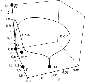
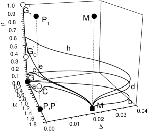
Figure 1: Static (left picture) and dynamic (right picture) flows of disordered model C for $n=1$ ($n<n_{c}$). Filled circles mean unstable FPs with $\gamma^{*}=0$, blank circles indicate projections of unstable FPs with nonzero $\gamma^{*}$, while the filled square denotes the stable FP.

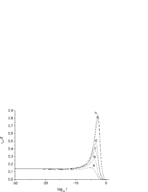
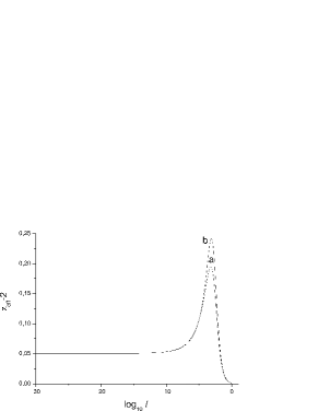
Figure 2: Dependencies of the effective dynamical exponent on the flow parameter for OP dimension $n=1$ and $n=3$. Curves are obtained on the basis of flows of Fig. 1 and Fig. 4.

It is interesting to look at contributions of different origin to the effective dynamical critical exponent $z_{\rm eff}$. They are shown in Fig. 3 for flows a and h of Fig.1 correspondingly. The contributions consist of (i) the terms already present in model A (dashed curve in Fig. 3), (ii) terms present in pure model C only (short dashed curve) and (iii) terms present in the diluted model C only (dashed-short dashed curve) [3]. The interplay of the above contributions gives the full effective exponent $z_{\rm eff}$ (solid line) and may lead to an almost asymptotic value of the exponent although the parameters are far away from asymptotics. This is an important point, since the appearance of an asymptotic value in one physical quantity does not mean that other quantities have also reached the asymptotics. This is due to the different dependence of physical quantities on the model parameters.

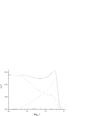
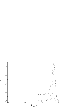
Figure 3: Different contributions to the effective dynamical critical exponent corresponding to the flows a and h of Fig. 1. The solid line represents the complete $z_{\rm eff}$, for the other lines see the text.

The second important case we consider here is the Heisenberg systems $n=3$. In asymptotics their critical behaviour is characterized by the FP P. The static flows and projections of the dynamic flows in this case are shown in Fig. 4. There exists a considerable difference to the one-loop picture. In the one-loop approximation the stable FP P is marginal: for this FP every value of $\rho^{*}$ between 0 and 1 is allowed. Therefore starting from different initial values flows approach different $\rho^{*}$. In contrast, Fig. 4 shows that within two-loop approximation all flows remain near the initial values of $\rho$. Only when the flows reach the region $u=u^{*}$, $\Delta=0$, $\rho$ drops down to its FP value $\rho^{*}=0$. This may be attributed to the marginality in one-loop order. The behaviour of $z_{\rm eff}$ corresponding to flow a of Fig. 4 is shown in right picture of Fig. 2. We present the dependencies of the effective dynamical critical exponent on the flow parameter only for one set of values $\gamma(\ell_{0})$ and $\rho(\ell_{0})$ (but for two different ratios $u(\ell_{0})/\Delta(\ell_{0})$ ) because for other values $\gamma(\ell_{0})$ and $\rho(\ell_{0})$ we observe similar behaviour: the peak increases for larger $\gamma(\ell_{0})$ and/or $\rho(\ell_{0})$. The experimental investigations give for a disordered Heisenberg magnet a value of the critical exponent $z=2.3\pm 0.1$ [39], that is larger than the value of the dynamical exponent for pure model A with $n=3$ (in our case $z=2.05$). This might be a consequence of the measurements performed in the non-asymptotic region.

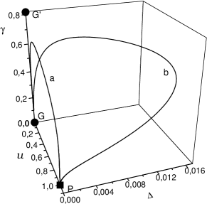
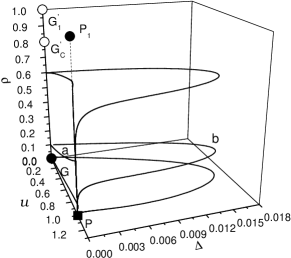
Figure 4: Static (left picture) and dynamic (right picture) flows of disordered model C for $n=3$ ($n>n_{c}$). Filled circles mean unstable FPs with $\gamma^{*}=0$, blank circles indicate projections of unstable FPs with nonzero $\gamma^{*}$, while the filled square denotes the stable FP.

5 Conclusions

We have studied the critical dynamics of model C in the presence of disorder.

Already one-loop order gives a qualitatively correct picture for suitable numbers of OP components $n$. In the asymptotics the conserved density is decoupled from the OP as it was expected. However the non-asymptotic critical behaviour of model C is strongly influenced by the presence of the static coupling between the OP and the conserved density as well as by the disorder. When approaching the asymptotic region the dynamical critical exponent usually shows a maximum starting from the van Hove value $z=2$ in the background. For the case $n<n_{c}$ $(n_{c}=4)$ the effective exponent might go after the maximum again through a minimum after it reaches its asymptotic value. It might be also the case that one observes the asymptotic value of the dynamical exponent although the parameters of the system are far from their asymptotic values. For systems with OP components $n>n_{c}$ only a maximum is observed.

These general observations remain qualitatively the same in two-loop approximation and are modified only quantitatively. In particular, the value of the marginal dimension $n_{c}$ lies between 1 and $2$ at $d=3$.

The existence of numerous FPs leads to a different cross-over behaviour of RG flows. Therefore the dynamical critical exponent can assume different values approaching asymptotics. For the case $n<n_{c}$ $z_{\rm eff}$ can either exceed the asymptotic value showing a peak or reaches its asymptotic value mechanically. For a system with order parameter dimension $n>n_{c}$ $z_{\rm eff}$ always shows a non-monotonous behaviour.

Appendix A Dynamical functionals and perturbation expansion

The model defined by expressions (1)-(8) within Bausch-Janssen-Wagner formulation [24] turns out to be described by an unrenormalized Lagrangian:

$${\mathcal{L}}=\int d^{d}xdt\Bigg{\{}{-}\mathring{\Gamma}\sum_{i=1}^{n}{\tilde{\varphi}_{0,i}}{\tilde{\varphi}_{0,i}}{+}\sum_{i=1}^{n}{\tilde{\varphi}_{0,i}}\left({\frac{\partial}{\partial t}}{+}\mathring{\Gamma}(\mathring{r}{-}\nabla^{2})\right)\varphi_{0,i}+\mathring{\lambda}_{m}\tilde{m}_{0}\nabla^{2}\tilde{m}_{0}$$

$$+\tilde{m}_{0}\left({\frac{\partial}{\partial t}}-a_{m}\mathring{\lambda}_{m}\nabla^{2}\right)m_{0}+\frac{1}{3!}\mathring{\Gamma}\mathring{u}\sum_{i}\tilde{\varphi}_{0,i}{\varphi}_{0,i}\sum_{j}{\varphi}_{0,j}{\varphi}_{0,j}$$

$$+\mathring{\Gamma}V(x)\sum_{i}\tilde{\varphi}_{0,i}(x,t){\varphi}_{0,i}(x,t)+\mathring{\Gamma}\mathring{\gamma}_{m}m_{0}\sum_{i}\tilde{\varphi}_{0,i}{\varphi}_{0,i}$$

$${-}\frac{1}{2}\mathring{\lambda}_{m}\mathring{\gamma}_{m}\tilde{m}_{0}\sum_{i}\nabla^{2}{\varphi}_{0,i}{\varphi}_{0,i}\Bigg{\}}$$ (46)

with new auxiliary response fields ${\tilde{\varphi}}_{i}(x,t)$. There are two ways to average over the random potential of disorder $V(x)$ for dynamics. The first way is the same as in statics and consists in using the replica trick [23], where $N$ replicas of the system are introduced in order to facilitate configurational averaging of the corresponding generating functional. Finally the limit $N\to 0$ has to be taken.

However it was established [25] that renormalization of the replicated Lagrangian leads to the same results as the renormalization of an Lagrangian obtained avoiding the replica trick but taking the mean of the Lagrangian (A) with respect to the random potential with distribution (8). The Lagrangian obtained in this way can be written in the form

$${\mathcal{L}}={\mathcal{L}}_{0}+{\mathcal{L}}_{int}\,,$$ (47)

where the Gaussian part ${\mathcal{L}}_{0}$ is given by (2.1) and ${\mathcal{L}}_{int}$ by (2.1). We perform the calculations on the basis of the Lagrangian defined by (47) using the Feynman graph technique.

Response propagators for OP $G(k,\omega)$ and secondary density $H(k,\omega)$ are equal to

$$G(k,\omega)=1/(-i\omega+\mathring{\Gamma}(\mathring{\tilde{r}}+k^{2}))\qquad\mbox{and}\qquad H(k,\omega)=1/(-i\omega+a_{m}\mathring{\lambda}_{m}k^{2})\,,$$ (48)

while the correlation propagators $C(k,\omega)$ and $D(k,\omega)$ are equal to

$$C(k,\omega)=2\mathring{\Gamma}/|-i\omega+\mathring{\Gamma}(\mathring{\tilde{r}}+k^{2})|^{2}\qquad\mbox{and}\qquad D(k,\omega)=2\mathring{\lambda}_{m}k^{2}/|-i\omega+a_{m}\mathring{\lambda}_{m}k^{2}|^{2}\,.$$ (49)

We proceed within two-loop approximation. In order to obtain the two-point vertex function ${{\mathring{\Gamma}_{\tilde{\varphi}\varphi}}}^{i,j}(\mathring{\tilde{r}},\mathring{\tilde{u}},\mathring{\Delta},\mathring{\gamma}_{m},\mathring{\Gamma},\mathring{\lambda}_{m},a_{m},k,\omega)={\mathring{\Gamma}_{\tilde{\varphi}\varphi}}(\mathring{\tilde{r}},\mathring{\tilde{u}},\mathring{\Delta},\mathring{\gamma}_{m},\mathring{\Gamma},\mathring{\lambda}_{m},a_{m},k,\omega)\delta_{i,j}$ one needs to calculate diagrams of corresponding order. The result of the calculations can be expressed in the form:

$$\mathring{\Gamma}_{\tilde{\varphi}\varphi}(\xi,k,\omega)=-i\omega\mathring{\Omega}_{\tilde{\varphi}\varphi}(\xi,k,\omega)+\mathring{\Gamma}^{st}_{{\varphi}\varphi}(\xi,k)\mathring{\Gamma}.$$ (50)

Here we introduce the correlation length $\xi(\mathring{\tau},\mathring{u},\mathring{\Delta})$, which is defined by

$$\xi^{2}=\left.\frac{\partial\ln\mathring{\Gamma}^{st}_{\varphi\varphi}}{\partial k^{2}}\right|_{k^{2}=0}.$$ (51)

The function $\mathring{\Gamma}_{{\varphi}\varphi}$ is the static two-loop vertex function of a disordered magnet. The structure (50) of the dynamic vertex function of pure model C was obtained in [28].

We can express the two-loop dynamical function $\mathring{\Omega}_{\tilde{\varphi}\varphi}$ in the form:

$$\mathring{\Omega}_{\tilde{\varphi}\varphi}(\xi,k,\omega)=1+\mathring{\Omega}^{1}_{\tilde{\varphi}\varphi}(\xi,k,\omega)+\mathring{\Omega}^{2}_{\tilde{\varphi}\varphi}(\xi,k,\omega),$$ (52)

where the one loop contribution has the structure

$$\mathring{\Omega}^{1}_{\tilde{\varphi}\varphi}(\xi,k,\omega)=4\mathring{\Delta}\mathring{\Gamma}\int_{k^{\prime}}\frac{1}{(-i{\omega}+\mathring{\Gamma}(\xi^{-2}+k^{\prime 2}))(\xi^{-2}{+}k^{\prime 2})}+{\gamma}\mathring{\Gamma}I_{C}(\xi,k,\omega),$$ (53)

while the two-loop contribution is of the form:

$$\mathring{\Omega}^{2}_{\tilde{\varphi}\varphi}(\xi,k,\omega)=\frac{n+2}{18}\mathring{\Gamma}{\mathring{u}}^{2}{\mathring{W}}^{(A)}_{{\tilde{\varphi}}\varphi}(\xi,k,\omega)-\frac{n+2}{3}\mathring{\Gamma}{\mathring{u}}{{\mathring{\gamma}}^{2}}{\mathring{C}}^{(T3)}_{{\tilde{\varphi}}\varphi}(\xi,k,\omega)+\mathring{\Gamma}{{\mathring{\gamma}}^{4}}{\mathring{S}}_{{\tilde{\varphi}}\varphi}(\xi,k,\omega)-$$

$$4\frac{n{+}2}{3}\mathring{\Gamma}{\mathring{u}}{\mathring{\Delta}}{\mathring{W}}^{(CD2)}_{{\tilde{\varphi}}\varphi}(\xi,k,\omega){+}16\mathring{\Gamma}{\mathring{\Delta}}^{2}\left({\mathring{W}}^{(CD3)}_{{\tilde{\varphi}}\varphi}(\xi,k,\omega){+}{\mathring{W}}^{(CD4)}_{{\tilde{\varphi}}\varphi}(\xi,k,\omega)\right){+}$$

$$4\mathring{\Gamma}{\mathring{\Delta}}{\mathring{\gamma}}^{2}\left({\mathring{W}}^{(CD5)}_{{\tilde{\varphi}}\varphi}(\xi,k,\omega)+{\mathring{W}}^{(CD6)}_{{\tilde{\varphi}}\varphi}(\xi,k,\omega)+2{\mathring{W}}^{(CD7)}_{{\tilde{\varphi}}\varphi}(\xi,k,\omega)\right),$$ (54)

with the rescaled coupling $\mathring{\gamma}=\mathring{\gamma}_{m}/{\sqrt{a_{m}}}$.

Expressions for the integral $I_{C}$ and for ${\mathring{W}}^{(A)}$, ${\mathring{C}}^{(T3)}$ and ${\mathring{S}}$ of pure model C are given in Appendix A.1 in Ref. [10], the contributions ${\mathring{W}}^{(CDi)}$ are the following:

$${\mathring{W}}_{{\tilde{\varphi}}\varphi}^{(CD2)}(\xi,k,\omega)=\int_{k^{\prime}}\int_{k^{\prime\prime}}\frac{1}{(\xi^{-2}+k^{\prime 2})(\xi^{-2}+k^{\prime\prime 2})(\xi^{-2}+(k+k^{\prime}+k^{\prime\prime})^{2})}$$

$$\times\frac{1}{(-i\omega+\mathring{\Gamma}(\xi^{-2}+(k+k^{\prime}+k^{\prime\prime})^{2}))},$$ (55)

$${\mathring{W}}_{{\tilde{\varphi}}\varphi}^{(CD3)}(\xi,k,\omega)=\int_{k^{\prime}}\int_{k^{\prime\prime}}\frac{\mathring{\Gamma}}{(\xi^{-2}+k^{\prime\prime 2})(-i\omega+\mathring{\Gamma}(\xi^{-2}+k^{\prime 2}))^{2}(-i\omega+\mathring{\Gamma}(\xi^{-2}+k^{\prime\prime 2}))},$$ (56)

$${\mathring{W}}_{{\tilde{\varphi}}\varphi}^{(CD4)}(\xi,k,\omega)=\int_{k^{\prime}}\int_{k^{\prime\prime}}\frac{1}{(\xi^{-2}+k^{\prime 2})(-i\omega+\mathring{\Gamma}(\xi^{-2}+(k+k^{\prime}+k^{\prime\prime})^{2}))}$$

$$\times\Bigg{[}\frac{1}{(\xi^{-2}+k^{\prime\prime 2})}\left(\frac{1}{(\xi^{-2}+(k+k^{\prime}+k^{\prime\prime})^{2})}+\frac{\mathring{\Gamma}}{-i\omega+\mathring{\Gamma}(\xi^{-2}+k^{\prime\prime 2})}\right)$$

$$+\frac{{\mathring{\Gamma}}^{2}}{(-i\omega+\mathring{\Gamma}(\xi^{-2}+k^{\prime 2}))(-i\omega+\mathring{\Gamma}(\xi^{-2}+k^{\prime\prime 2}))}\Bigg{]},$$ (57)

$${\mathring{W}}_{{\tilde{\varphi}}\varphi}^{(CD5)}(\xi,k,\omega){=}\!\int_{k^{\prime}}\!\!\int_{k^{\prime\prime}}\!\!\frac{{\mathring{\Gamma}}^{2}}{(\xi^{-2}{+}k^{\prime\prime 2})({-}i\omega{+}\mathring{\Gamma}(\xi^{-2}{+}k^{\prime 2}))^{2}}$$

$$\times\frac{1}{({-}i\omega{+}\mathring{\Gamma}(\xi^{-2}{+}k^{\prime\prime 2}){+}\mathring{\lambda}(k^{\prime}{+}k^{\prime\prime})^{2})},$$ (58)

$${\mathring{W}}_{{\tilde{\varphi}}\varphi}^{(CD6)}(\xi,k,\omega){=}\int_{k^{\prime}}\int_{k^{\prime\prime}}\frac{{\mathring{\Gamma}}^{2}}{(\xi^{-2}{+}k^{\prime\prime 2})(-i\omega{+}\mathring{\Gamma}(\xi^{-2}{+}k^{\prime 2}){+}\mathring{\lambda}(k{+}k^{\prime})^{2})^{2}}$$

$$\times\frac{1}{(-i\omega{+}\mathring{\Gamma}(\xi^{-2}{+}k^{\prime\prime 2}){+}\mathring{\lambda}(k{+}k^{\prime})^{2})},$$ (59)

$${\mathring{W}}_{{\tilde{\varphi}}\varphi}^{(CD7)}(\xi,k,\omega)=\int_{k^{\prime}}\int_{k^{\prime\prime}}\frac{1}{(\xi^{-2}+(k+k^{\prime}+k^{\prime\prime})^{2})(-i\omega+\mathring{\Gamma}(\xi^{-2}+k^{\prime 2}))}$$

$$\times\frac{1}{(-i\omega+\mathring{\Gamma}(\xi^{-2}+k^{\prime\prime 2})+\mathring{\lambda}(k^{\prime}+k^{\prime\prime})^{2})}$$

$$\times\Bigg{[}\frac{\mathring{\Gamma}}{(\xi^{-2}+k^{\prime 2})}+\frac{{\mathring{\Gamma}}^{2}}{(-i\omega+\mathring{\Gamma}(\xi^{-2}+(k+k^{\prime}+k^{\prime\prime})^{2})+\mathring{\lambda}(k^{\prime}+k^{\prime\prime})^{2})}\Bigg{]},$$ (60)

where we use rescaling $\mathring{\lambda}=a_{m}\mathring{\lambda}_{m}$.

Appendix B Renormalizing factors

We use the minimal subtraction RG scheme [29] for renormalization. In the definition of the renormalizing factors we follow Ref. [10].

For renormalization of the OP $\vec{\varphi}$, fourth-order couplings $u,\,\Delta$ and correlation functions with $\varphi^{2}$ insertion we introduce the renormalizing factors $Z_{\varphi}$, $Z_{u}$, $Z_{\Delta}$ and $Z_{\varphi^{2}}$ respectively via the relations:

$$\vec{\varphi}_{0}=Z^{1/2}_{\varphi}\vec{\varphi},\quad{\mathring{u}}=\mu^{\varepsilon}Z_{\varphi}^{-2}Z_{u}uA_{d}^{-1},\quad{\mathring{\Delta}}=\mu^{\varepsilon/2}Z_{\varphi}^{-2}Z_{\Delta}\Delta A_{d}^{-1},\quad\frac{1}{2}|\varphi_{0}|^{2}=Z_{\varphi^{2}}\frac{1}{2}|\varphi|^{2},$$ (61)

where $\mu$ is the scale and $\varepsilon=4-d$.

The renormalization of $\mathring{r}$ is performed via the relation

$${\mathring{r}}=Z_{\varphi}^{-1}Z_{r}r.$$ (62)

The renormalizing factor $Z_{r}$ is connected to $Z_{\varphi^{2}}$ by the relation $Z_{\varphi^{2}}=Z_{\varphi}^{-1}Z_{r}$ therefore within minimal subtraction scheme one does not need to consider renormalization for correlation functions containing $\varphi^{2}$ insertions explicitly. However a correlation function containing two insertions $<\varphi^{2}\varphi^{2}>$ needs additive renormalization $A_{\varphi^{2}}$.

The renormalization of dynamic quantities is introduced similar to statics. Renormalizing factors for the dynamic field $\vec{\tilde{\varphi}}$, $Z_{\tilde{\varphi}}$, and kinetic coefficient $\Gamma$, $Z_{\Gamma}$, are introduced via

$$\vec{\tilde{\varphi}}_{0}{=}Z^{1/2}_{\tilde{\varphi}}\vec{\tilde{\varphi}},\quad\mathring{\Gamma}{=}Z_{\Gamma}\Gamma.$$ (63)

The factor $Z_{\Gamma}$ in the last equation contains a static contribution $Z_{\varphi}$, which can be separated:

$$Z_{\Gamma}=Z_{\varphi}^{1/2}Z_{\tilde{\varphi}}^{-1/2}Z^{(d)}_{\Gamma}.$$ (64)

Since in the dynamic model mode coupling terms are absent $Z_{\Gamma}^{(d)}=1$. Therefore

$$Z_{\Gamma}=Z_{\varphi}^{1/2}Z_{\tilde{\varphi}}^{-1/2}.$$ (65)

In model C one needs to introduce additional renormalizing factors for the secondary density $m$ and its coupling parameter $\gamma$. They are renormalized similar to $\varphi$ and $u$ in Eq. (61):

$$a_{m}^{1/2}m_{0}=Z_{m}m,\quad a_{m}^{-1/2}{\mathring{\gamma}}_{m}=\mu^{\varepsilon/2}Z_{\varphi}^{-1}Z_{m}^{-1}Z_{\gamma}\gamma A_{d}^{1/2}.$$ (66)

There are relations connecting the static $Z$-factors of model C to the static $Z$-factors of the Landau-Ginzburg-Wilson model by integrating out the secondary field $m$ in the Hamiltonian (5). Thus the renormalizing factor of $\gamma$ is determined by:

$$Z_{\gamma}=Z^{2}_{m}Z_{\varphi}Z_{\varphi^{2}}.$$ (67)

Therefore Eq. (66) can be rewritten as

$$a_{m}^{-1/2}{\mathring{\gamma}}_{m}=\mu^{\varepsilon/2}Z_{\varphi^{2}}Z_{m}\gamma A_{d}^{-1/2}.$$ (68)

The additive renormalization $A_{\varphi^{2}}$ of the specific heat of the Landau-Ginzburg-Wilson model determines the renormalizing factor $Z_{m}$ via the relation

$$Z_{m}^{-2}(u,\Delta,\gamma)=1+\gamma^{2}A_{\varphi^{2}}(u)$$ . (69)

Since the secondary density is conserved, no new renormalizing factor is needed for the dynamic auxiliary density $\tilde{m}$. It renormalizes by:

$$a_{m}^{-1/2}{\tilde{m}}_{0}=Z_{m}^{-1}\tilde{m}$$ . (70)

The kinetic coefficient $\lambda$ renormalizes as

$$a_{m}{\mathring{\lambda}}_{m}=Z_{\lambda}\lambda.$$ (71)

Similar to $Z_{\Gamma}$ its static contribution can be separated:

$$Z_{\lambda}=Z^{2}_{m}Z_{\lambda}^{(d)}.$$ (72)

Since no mode coupling terms are present in model C, $Z_{\lambda}^{(d)}=1$, therefore

$$Z_{\lambda}=Z^{2}_{m}.$$ (73)

Renormalizing $\mathring{\Gamma}_{\tilde{\varphi}\varphi}$ we obtain the two-loop renormalizing factor $Z_{\tilde{\varphi}}$ in the form:

$$Z_{\tilde{\varphi}}=1{-}8\frac{\Delta}{\varepsilon}-2\frac{\gamma^{2}}{\varepsilon}\frac{w}{1+w}+\frac{1}{\varepsilon^{2}}\Big{[}\left({\gamma^{2}}\frac{w}{1+w}\left(\frac{1}{w+1}-\left(\frac{n}{2}-1\right)\right)-\frac{n+2}{3}u\right){\gamma^{2}}\frac{w}{1+w}$$

$$+4\Delta{\gamma^{2}}\!\left(\!\frac{w}{1{+}w}\!\right)^{2}\!\!{+}20\Delta{\gamma^{2}}\frac{w}{1{+}w}\!+96\Delta^{2}{-}4\frac{n{+}2}{3}u\Delta\Big{]}{+}\frac{1}{2\varepsilon}\Bigg{\{}\!\Bigg{[}\frac{n{+}2}{3}u\left(\!\!1{-}3\ln\frac{4}{3}\!\right)$$

$${+}{\gamma^{2}}\!\frac{w}{1{+}w}\Bigg{(}\!\frac{n}{2}{-}\frac{w}{1{+}w}{-}\frac{3(n{+}2)}{2}\ln\frac{4}{3}{-}\frac{1{+}2w}{1{+}w}\ln\frac{(1{+}w)^{2}}{1{+}2w}\!\Bigg{)}\Bigg{]}{\gamma^{2}}\frac{w}{1{+}w}{+}3\frac{n{+}2}{3}u\Delta$$

$${-}44\Delta^{2}{-}12\Delta{\gamma^{2}}\frac{w}{1{+}w}\Bigg{\}}{-}\frac{n{+}2}{12}\frac{u}{\varepsilon}\left(\ln\frac{4}{3}{-}\frac{1}{12}\right){+}$$

$$4\frac{\Delta}{\varepsilon}{\gamma^{2}}\frac{w}{1+w}\left[\frac{w}{2}\ln\frac{w}{1+w}-\frac{3}{2}\ln(1+w)-\frac{1}{2}\frac{w}{1+w}\ln w\right]$$ (74)

References

References

• [1] For recent reviews see e.g.: R. Folk, Yu. Holovatch, T. Yavors’kii, Physics - Uspekhi 46 169 (2003) [Uspekhi Fizicheskikh Nauk 173 175], preprint cond-mat/0106468; A. Pelissetto, E. Vicari, Phys. Rep. 368 549 (2002), preprint cond-mat/0012164
• [2] A. B. Harris, J. Phys. C: Solid State Phys. 7, 1671 (1974)
• [3] This is the way in which the Harris criterion was originally formulated. However afterwards it has been often interpreted as a prediction of a change in asymptotic criticality if $\alpha_{pure}>0$. We thank W. Janke for attracting our attention to the original formulation and later sloppy interpretations of the Harris criterion. For the cases treated here when $\alpha_{pure}>0$ a new universality class is found.
• [4] C. Bervillier, Phys. Rev. B 34 8141 (1986); M. Dudka, Yu. Holovatch, T. Yavors’kii, J. Phys. Stud. 5 233 (2001).
• [5] B. I. Halperin, P. C. Hohenberg, and S.-k. Ma, Phys. Rev. B 10, 139 (1974).
• [6] U. Krey, Phys. Lett. 57A 215 (1976);
• [7] U. Krey, Z. Physik B 26, 355 (1977).
• [8] I. D. Lawrie, and V. V. Prudnikov, J. Phys. C 17, 1655 (1984).
• [9] R. Folk and G. Moser, Phys. Rev. Lett. 91, 030601 (2003)
• [10] R. Folk, G. Moser, Phys. Rev. E 69, 036101 (2004).
• [11] G.Grinstein, S.-k. Ma, and G. Mazenko, Phys. Rev. B 15 258 (1977).
• [12] V. V. Prudnikov, A. N. Vakilov, Sov. Phys. JETP 74, 990 (1992) [Zh. Eksp. Teor. Fiz. 101, 1853 (1992)].
• [13] K. Oerding and H. K. Janssen, J. Phys. A: Math. Gen. 28, 4271 (1995).
• [14] H. K. Janssen, K. Oerding, and E. Sengenspeick, J. Phys. A: Math. Gen. 28, 6073 (1995).
• [15] M. Dudka, R. Folk, Yu. Holovatch, and D. Ivaneiko, J. Magn. Magn. Mater. 53 243 (2003).
• [16] A. Perumal, V. Srinivas, V. V. Rao, R. A. Dunlap, Phys. Rev. Lett. 91 137202 (2003).
• [17] P. E. Berche, C.Chatelain, B. Berche, W. Janke, Eur. Phys. J. B, 39, 463 (2004)
• [18] P. Calabrese, P. Parruccini, A. Pelissetto, E. Vicari, Phys. Rev. E 69 036120 (2004).
• [19] B. Berche, P. E. Berche, C.Chatelain, W. Janke, Condens. Matter Phys. 8, 47 (2005)
• [20] D. E. Khmel’nitskii, Zh. Eksp. Teor. Fiz. 68 (1975) 1960 [ Sov. Phys. JETP 41 (1975) 981]; A. B. Harris, T. C. Lubensky, Phys. Rev. Lett. 33 (1974) 1540; T. C. Lubensky, Phys. Rev. B 11 (1975) 3573.
• [21] G. Grinstein, A. Luther, Phys. Rev. B 13 (1976) 1329.
• [22] B. I. Halperin, P. C. Hohenberg, Rev. Mod. Phys. 49, 436 (1977).
• [23] V. J. Emery, Phys. Rev. B 11, 239 (1975).
• [24] R. Bausch, H. K. Janssen, and H. Wagner, Z. Phys. B 24, 113 (1976).
• [25] C. De Dominicis, Phys. Rev. B 18, 4913 (1978).
• [26] R. Folk, Yu. Holovatch, T. Yavors’kii, Phys. Rev. B 61 15114 (2000); J. M. Carmona, A. Pelissetto, and E. Vicari Phys. Rev. B 61, 15136 (2000).
• [27] U.Krey, Z. Phys. B 26, 355 (1977).
• [28] R. Folk, G. Moser, Acta Physica Slovaca 52, 285 (2002).
• [29] G. ’t Hooft, M. Veltman, Nucl. Phys. B 44 (1972) 189; G. ’t Hooft, Nucl. Phys. B 61 (1973) 455.
• [30] M. Dudka, R. Folk, Yu. Holovatch, G. Moser, Phys. Rev. E 72 036107 (2005).
• [31] J. Kyriakidis and D. J. W. Geldart 53, 11572 (1996).
• [32] K. Wilson, M. E. Fisher, Phys. Rev. Lett. 28 (1972) 240.
• [33] R. Schloms and V. Dohm, Europhys. Lett. 3 (1987) 413; R. Schloms and V. Dohm, Nucl. Phys. B 328 (1989) 639.
• [34] G. A. Baker, Jr., B. G. Nickel, D. I. Meiron, Phys. Rev. B 17, (1978) 1365.
• [35] P. J. S. Watson, J. Phys. A 7 (1974) L167.
• [36] G. A. Baker, Jr., P. Graves-Morris, Padé Approximants (Addison-Wesley: Reading, MA, 1981)
• [37] N. Rosov, C. Hohenemser, M. Eibschütz, Phys. Rev. B 46, 3452 (1992).
• [38] Compare with their analytic form that can be obtained with the help of Eq. (4).
• [39] M. Alba, S. Pouget, J. Magn. Magn. Mater 226-330 542 (2001).