Exact Results for the Roughness of a Finite Size Random Walk

Abstract

We consider the role of finite size effects on the value of the effective Hurst exponent $H$. This problem is motivated by the properties of the high frequency daily stock-prices. For a finite size random walk we derive some exact results based on Spitzer’s identity. The conclusion is that finite size effects strongly enhance the value of $H$ and the convergency to the asymptotic value ($H=1/2$) is rather slow. This result has a series of conceptual and practical implication which we discuss.

, , , ,

1 Introduction

The dynamics of stock-prices can be described as a subtle form of random walk with complex properties and correlations. The main characteristics which are usually considered are the broad distribution of price returns (fat tails) and the clustering of volatility [bib1, , bib2, , bib3, ]. Recently, also the roughening properties, defined by the Hurst exponent $H$ bib4 , have been considered bib5 , bib6 , bib7 . The idea is that the roughening exponent can provide information which goes beyond the above two properties. However, the extraction of this information is not simple and the usual interpretation of deviation from the random walk value ($H=1/2$) is in terms of generic long range correlations. Sometimes the Hurst exponent is simply used as a generic statistical indicator without particular interpretation bib8 . Here we show that finite size effects in the real data can alter significantly the determination of the effective Hurst exponent. In fact, high frequency stock-price data are relatively homogeneous within the same day, but the large night jump (often of the order of the total daily fluctuation), implies an intrinsic limit on the size of the dataset bib14 . Motivated by these observations we consider how finite size effects affect the determination of the Hurst exponent for a finite size random walk. We derive exact results for the expectation value of the maximum value of a random walk using the Spitzer’s identity bib12 . From this one can derive the effective Hurst exponent for the case in which the vertical fluctuation is defined by the maximum and the minimum values. There are also different methods to estimate $H$ but we believe that, especially for financial data, the one based on the maximum and the minimum values is especially relevant because of the role played by these values in various trading strategies.
The main result is that the effective Hurst exponent is strongly enhanced by finite size effects and that the convergency to the asymptotic value $H=1/2$ is rather slow. This result will be further enhanced by the inclusion of “fat tails” and non-stationary properties. This implies that high frequency daily stock-prices are unavoidably affected by finite size effects bib14 . In addiction non-stationarity can make the convergency much slower providing a possible alternative interpretation of the deviations from $H=1/2$ which are observed in long time series.

2 Exact analysis of a Finite Size Random Walk

In this section we derive some exact result for finite Random Walks which are necessary in order to consider the roughness properties for a finite size system. Suppose that ${\delta x_{1},\delta x_{2},...,\delta x_{n}}$ are independent random variables, each taking the value $+1$ with probability $p$, and $-1$ otherwise. Consider the sums:

$$X_{n}=\sum_{i=1}^{n}\delta x_{i}$$ (1)

then the sequence $X=\{X_{i}:i\geq 0\}$ is a simple random walk starting at the origin. In order to compute the expectation value of the maximum and the minimum of the walk after $n$ steps, is useful to consider the following theorem.

Theorem 1 (Spitzer’s identity)

bib12 Assume that $X$ is a right-continuous random walk, and let $M_{n}=\max\,\{X_{i}:0\geq i\geq n\}$ be the maximum of the walk up to time $n$. Then, introducing the auxiliary variables $s$ and $t$, for $|s|,|t|<1$ one has Eq.2,

$$\log\Big{(}\sum_{n=0}^{\infty}\,t^{n}\,\mathbb{E}(s^{M_{n}})\Big{)}=\sum_{n=1}^{\infty}\frac{1}{n}\,t^{n}\,\mathbb{E}\,(s^{X_{n}^{+}})$$ (2)

where $X_{n}^{+}=\max\,\{0,X_{n}\}$ and $\mathbb{E}$ is the expectation value.

Considering the exponential of both member of Eq.2 one has:

$$\sum_{n=0}^{\infty}\,t^{n}\,\mathbb{E}(s^{M_{n}})=\exp\Big{(}\sum_{n=1}^{\infty}\frac{1}{n}\,t^{n}\,\mathbb{E}\,(s^{X_{n}^{+}})\Big{)}$$ (3)

The $k$-derivative with respect to $t$ of the left hand side of Eq.3 for $t=0$, gives:

$$\frac{{\partial}^{k}}{\partial t^{k}}{\Bigg{|}}_{0}=k!\;\mathbb{E}(s^{M_{k}})$$ (4)

Defining the right side member of Eq.3 as $f(t)$ one can derive:

$$\frac{{\partial}^{k}}{\partial t^{k}}f(t){\Bigg{|}}_{0} = \sum_{j=1}{k}\frac{(k-1)!}{(k-j)!}\mathbb{E}(s^{X_{j}^{+}})\Bigg{(}\frac{{\partial}^{(k-j)}}{\partial t^{(k-j)}}f(t)\Bigg{)}{\Bigg{|}}_{0}$$

$$f(0) = 1$$ (5)

By equating Eq.4 and Eq.5 one obtains:

$$\mathbb{E}(s^{M_{k}})=\frac{1}{k}\sum_{j=1}^{k}\frac{\mathbb{E}(s^{X_{j}^{+}})}{(k-j)!}\Bigg{(}\frac{{\partial}^{(k-j)}}{\partial t^{(k-j)}}f(t)\Bigg{)}{\Bigg{|}}_{0}$$ (6)

In order to obtain $\mathbb{E}(M_{k})$ from the function $\mathbb{E}(s^{M_{k}})$ it is useful to consider the following expansion which holds for a symmetrical probability density function:

$${\mathbb{E}} (s^{X_{j}^{+}})=\int_{-\infty}^{\infty}s^{X_{j}^{+}}P_{j}(X_{j})\,dX_{j}$$

$$= \int_{-\infty}^{0}P_{j}(X_{j})\,dX_{j}+\int_{0}^{\infty}s^{X_{j}}P_{j}(X_{j})\,dX_{j}$$

$$= \frac{1}{2}+\int_{0}^{\infty}s^{X_{j}}P_{j}(X_{j})\,dX_{j}$$

$$\simeq \frac{1}{2}+\int_{0}^{\infty}(1+X_{j}\ln(s)+\frac{1}{2}X_{j}^{2}{(\ln(s))}^{2}+...)P_{j}(X_{j})\,dX_{j}$$

$$\simeq 1+\ln(s)\int_{0}^{\infty}X_{j}P_{j}(X_{j})\,dX_{j}+{{\mathcal{O}}}{(\ln(s))}^{2}$$

$$= 1+\frac{1}{2}\,\mathbb{E}(|X_{j}|)\,\ln(s)+{\mathcal{O}}{(\ln(s))}^{2}$$

We now insert this result into Eq. 6. Considering also the identity:

$$\mathbb{E}(M_{k})=\lim_{s\rightarrow 1}\frac{\mathbb{E}(s^{M_{k}})-1}{\ln(s)}$$ (8)

we finally obtain:

$$\mathbb{E}(M_{k})=\sum_{i=1}^{k}\frac{\mathbb{E}(|X_{i}|)}{2i}$$ (9)

Now we consider various possibilities for the specific nature of the random walk:

a)

If the increments $\delta x$ are independent and corresponding to a gaussian distribution with $\mathbb{E}(\delta x)=0$ and variance $\sigma^{2}=1$, one obtains:

$$\mathbb{E}(|X_{i}|) = \sqrt{\frac{2i}{\pi}}$$ (10)

b)

If $\delta x$ have values $\pm 1$ with equal probability one gets:

$$\mathbb{E}(|X_{i}|) = \sum_{X_{i}=-i}^{i}|X_{i}|P_{i}(X_{i})$$ (11)

where

$$P_{i}(X_{i})={i\choose{\frac{X_{i}+i}{2}}}{\Bigg{(}\frac{1}{2}\Bigg{)}}^{i}$$ (12)

This leads to

$$\mathbb{E}(|X_{i}|) = \Bigg{\{}\begin{array}[]{ll}\frac{(i-1)!!}{(i-2)!!}\qquad\mbox{if $i$ is even}\\ \frac{(i)!!}{(i-1)!!}\qquad\mbox{if $i$ is odd}\end{array}$$ (15)

These explicit results permit now to compute the exact expectation for finite size random walk properties. Note that Eq.9 has a general value with the only assumption that the increments are not correlated and symmetrically distributed. This means, for example, that one could test the properties of stock-prices for finite size samples being able to separate the role of fat tail, included in Eq.9, from the role of correlations. In the present paper we use Eq.9 to estimate the effective roughness exponent of finite size systems.

3 Effective roughness for a finite size Random Walk

Equation Eq.9 gives an exact result relation between the expectation value of the maximum value $M_{k}$ of a symmetric random walk of $k$ steps, for a given probability distribution $\mathbb{E}(|X_{i}|)$ of the individual step. In terms of Monte Carlo simulations this would correspond to an infinite number of samples. Since the Monte Carlo method will be applied also to cases for which the analytical result is not available, we can use the present case as a test for the convergency of the Monte Carlo method.
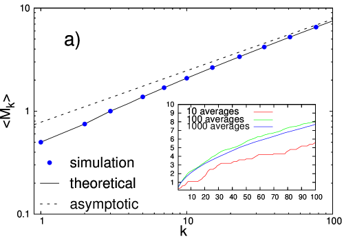
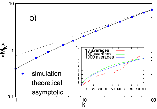
This comparison is shown in Fig.1 (a and b) where the two inserts show precisely the degree of convergency as a function of the samples considered.

Figure 1: The log-log graph shows $\mathbb{E}(M_{k})$ as a function of $k$ in the case of a) random walk with two identical steps and b) Gaussian random walk. In the inserts we show the convergency of the simulations to expected value as a function of the number of realizations considered.

In order to estimate the effective roughness exponent as a function of the size of the interval considered, we can compute the maximum fluctuation in a given interval of size $n$:

$$R(n)=\mathbb{E}(\max(n))-\mathbb{E}(\min(n))$$ (16)

and estimate the effective Hurst exponent $H$ from the scaling relation:

$$R(n)\simeq n^{H(n)}$$ (17)

For $n\rightarrow\infty$ we expect to recover the standard random walk result $H(n\rightarrow\infty)=1/2$.

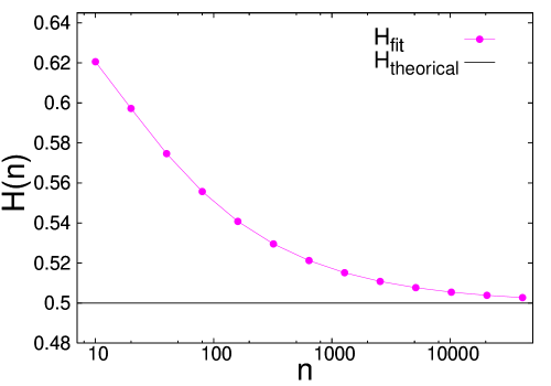
In Fig.2 we report the effective Hurst exponent $H(n)$ as a function of the size $n$ of the interval considered. One can see that for finite value of $n$ the value of $H(n)$ is always larger than the asymptotic value $H=1/2$ and that the convergency to the asymptotic value is rather slow.

Figure 2: This plot shows the trend obtained fitting the curve ${\mathcal{R}}(n)$ for different values of the size $n$. The results shows an overestimate of Hurst exponent for small size, due to finite size effects. This is a general result and it shows that finite size effects always enhance the apparent Hurst exponent. This enhancement can be understood by considering that, in some sense,a single step would correspond to $H=1$, so the asymptotic value $H=1/2$ is approached from above.

This result has a number of implications:

(i)

Usually a deviation of the value of $H$ from $1/2$ is interpreted in terms of long range correlations bib8 . We can see that a positive deviation $H>1/2$ can instead be due to finite size effects. This result is especially relevant for high frequency stock-prices data. In this case in fact the data are statistically homogeneous only within a single day because the night jump is usually very large bib14 . The typical number of transactions, for stocks of intermediate volatility, ranges between $500$ and $3000$. In order to have a statistical significance the maximum interval considered for the estimate of $H$ should not exceed one tenth of their total number. The interval if scaled to be considered ranges therefore from a few transactions to about $100$ bib14 . From Fig.2 we can see that this would correspond to appreciable deviation from $H=1/2$.

(ii) Fat Tails and Short Range Correlations.

Usually stock-price dynamics does not show short range correlations. However, in case these would be present, their effect would be to decrease the effective number of independent steps, enhancing therefore the of finite size effects. A much more important implication of the same type is due to the fat tails distributions of returns. In fact, in presence of a broad distribution of step size, the few large steps will play a major role and the finite size effects will be strongly enhanced. We are going to see that this point is very relevant for the analysis of high frequency stock-price data bib14 .

(iii) Non-stationarity.

The present analysis of finite size effects on the roughness is performed under the hypothesis of a stationary process. It is well known instead that economic data show marked deviation from stationarity. This implies that the convergency to the asymptotic value $H=1/2$ can be much slower if one includes these effects. In this perspective even data which refer to very long series may not reach convergency due to non stationarity. This implies a possible alternative origin for the deviation from $1/2$ which have been reported for long time seriesbib14 . In the future we intend to consider specific models to test this possibility.

References

- [1] B. Mandelbrot, Fractals and Scaling in Finance, Springer Verlag, New York, 1997.
- [2] R.N. Mantegna, H.E. Stanley, An Introduction to Econophysics, Cambridge University Press, Cambridge, 2000.
- [3] J.P. Bouchaud, Theory of Financial Risk, Cambridge University Press, Cambridge, 2000.
- [4] H.E. Hurst, Long-term storage capacity reservoirs, Transaction of the American Society of Civil Engineers 116, 770-808, 1951.
- [5] S.O. Cajueiro, B. Tabak, The Hurst exponent over time: testing the assertion that emerging market are becoming more efficient, Physica A, vol. 336, pag. 521-537, 2004.
- [6] D. Grech, Z. Mazur, Can one make any crash prediction in finance using the local Hurst exponent idea?, Physica A, vol. 336, pag. 133-145, 2004.
- [7] A. Carbone, G. Castelli, H.E. Stanley, Time-dependent Hurst exponent in financial time series, Physica A, vol. 344, pag. 267-271, 2004.
- [8] T. Di Matteo, T. Aste, M.M. Dacorogna, Long-term memories of developed and emerging markets: Using the scaling analysis to characterize their stage of development, Journal of Banking and Finance, vol. 29, pag. 827-851, 2005.
- [9] G. Grimmet, D. Stirzaker, Probability and Random Processes, Oxforf University Press, Oxford, 2001.
- [10] V. Alfi, F. Coccetti, M. Marotta, A.Petri, L.Pietronero, Roughness and Finite Size Effect in the NYSE Stock-Price Fluctuations, printing in 2006.