Dielectric response of a polar fluid trapped in a spherical nanocavity

Abstract

We present extensive Molecular Dynamics simulation results for the structure, static and dynamical response of a droplet of 1000 soft spheres carrying extended dipoles and confined to spherical cavities of radii $R=2.5$, 3, and 4 nm embedded in a dielectric continuum of permittivity $\epsilon^{\prime}\geq 1$. The polarisation of the external medium by the charge distribution inside the cavity is accounted for by appropriate image charges. We focus on the influence of the external permittivity $\epsilon^{\prime}$ on the static and dynamic properties of the confined fluid. The density profile and local orientational order parameter of the dipoles turn out to be remarkably insensitive to $\epsilon^{\prime}$. Permittivity profiles $\epsilon(r)$ inside the spherical cavity are calculated from a generalised Kirkwood formula. These profiles oscillate in phase with the density profiles and go to a “bulk” value $\epsilon_{b}$ away from the confining surface; $\epsilon_{b}$ is only weakly dependent on $\epsilon^{\prime}$, except for $\epsilon^{\prime}=1$ (vacuum), and is strongly reduced compared to the permittivity of a uniform (bulk) fluid under comparable thermodynamic conditions.

The dynamic relaxation of the total dipole moment of the sample is found to be strongly dependent on $\epsilon^{\prime}$, and to exhibit oscillatory behaviour when $\epsilon^{\prime}=1$; the relaxation is an order of magnitude faster than in the bulk. The complex frequency-dependent permittivity $\epsilon(\omega)$ is sensitive to $\epsilon^{\prime}$ at low frequencies, and the zero frequency limit $\epsilon(\omega=0)$ is systematically lower than the “bulk” value $\epsilon_{b}$ of the static primitivity.

I Introduction

Following the pioneering work of Debye Debye (1929), Kirkwood Kirkwood (1939), and Onsager Onsager (1936), the bulk dielectric response of polar materials is by now well understood Madden and Kivelson (1984), and dielectric response is a method of choice for the experimental investigation of molecular dynamics in condensed matter. Simulations of model polar systems have played a key role in our understanding of dielectric fluids Weis and Levesque (2005), and the subtle problems arising in the simulation of finite, but periodically repeated samples of such fluids, linked to the proper handling of boundary conditions, have been clarified in the eighties Neumann (1983); Neumann and Steinhauser (1983). However, with few exceptions Bagchi and Chandra (1991); Senapati and Chandra (1999); Teschke et al. (2001); Stern and Feller (2003); Ballenegger and Hansen (2003, 2005), much less experimental, theoretical and numerical effort has gone into understanding the dielectric response of confined polar fluids.

Consider a fluid of polar molecules trapped in a finite or infinite (along one or two directions) cavity surrounded by a dielectric material characterised by a permittivity different from that of the bulk polar fluid. The global dielectric response of the former is determined by the fluctuations and relaxation of the overall dipole moment of the trapped fluid. The question we wish to address is how the dipolar fluctuations are affected by confinement, i.e. by the presence of a surface separating the polar fluid from the dielectric material which surrounds the cavity. One can distinguish between two main effects due to the presence of such interfaces. The first is purely geometric: how are the dipolar fluctuations affected in the vicinity of a non-polarisable interface, compared to bulk fluctuations? In particular, can one define a meaningful local dielectric permittivity tensor $\tensor{\epsilon}(\vec{r})$, when the polar molecules are restricted to stay on one side of a confining surface, with vacuum on the other side. This question has been recently addressed in the case of simple geometries (slab or spherical cavity) Senapati and Chandra (1999); Ballenegger and Hansen (2005). The second effect arises from the electric boundary conditions which must be satisfied when the confining medium is polarisable, and hence characterised by a permittivity $\epsilon^{\prime}>1$. In this paper we investigate the second effect in the case of a simple polar fluid confined to a spherical cavity carved out of a dielectric continuum which extends to infinity in all directions. Note that in the limit where the system consists of a single polar molecule fixed at the centre of the spherical cavity, the system reduces to Onsager’s celebrated model for the calculation of the permittivity of a polar material Onsager (1936).

The model of a polar fluid in a spherical cavity may be regarded as a crude representation of dual physical situations. One concerns micro-emulsions where inverse micelles are nanodroplets of water in oil, which are stabilised by a monolayer of surfactants. The majority oil phase then provides the embedding dielectric medium. The conjugate situation is that of a globular macromolecule (i.e. a protein), made up of polar segments, dissolved in water. The connectivity of the macromolecule is then crudely accounted for by confining the unconnected polar residues to a spherical volume equal to that of the cavity. In that case the solvent (water) plays the role of the embedding continuum.

II Model and simulation methodology

Consider a system of $N$ polar molecules confined to a spherical cavity of radius $R$ surrounded by an infinite dielectric continuum of permittivity $\epsilon^{\prime}$. Following related earlier work Ballenegger and Hansen (2004, 2005) the model which will be investigated is one of spherical molecules carrying extended (rather than point) dipoles consisting of two opposite charges $\pm q$ displaced symmetrically by a distance $d/2$ from the centre of the molecule, such that the absolute dipole moment is $\mu=qd$. Let $\vec{r}_{i}$ be the position of the centre of the molecule $i$, and $\hat{\mu}_{i}$ be the unit vector along the dipole moment of that molecule. The two charges $q_{\pm}=\pm q$ are than placed at $\vec{r}_{i\pm}=\vec{r}_{i}\pm\frac{d}{2}\hat{\mu}_{i}$.

If $\phi(\vec{r},\vec{r}^{\prime})$ is the electrostatic potential at $\vec{r}^{\prime}$ due to a unit charge at $\vec{r}$, taking proper account of the electrostatic boundary conditions at the surface of the spherical cavity, then the total interaction energy of a pair of molecules $i$ and $j$ is:

$$v(\vec{r}_{i},\vec{r}_{j})=v_{0}(|\vec{r}_{i}-\vec{r}_{j}|)+\sum_{\alpha,\beta=\pm}q_{\alpha}q_{\beta}\phi(\vec{r}_{i\alpha},\vec{r}_{j\beta})$$ (1)

where $v_{0}(r)$ is the short-range repulsive potential between the spherical molecules, which is chosen to be of inverse power form as in Ballenegger and Hansen (2005):

$$v_{0}(r)=4u\left(\frac{\sigma}{r}\right)^{n}$$ (2)

with $n=12$ in practice.

The exact form of $\phi(\vec{r},\vec{r}^{\prime})$ for the spherical geometry is derived in the Appendix by solving Poisson’s equation with the appropriate electrostatic boundary conditions. This cumbersome expression is not well adapted to simulations, and may be replaced by the approximation:

$$\phi(\vec{r},\vec{r}^{\prime})=\frac{1}{4\pi\epsilon}\left[\frac{1}{|\vec{r}-\vec{r}^{\prime}|}+(1-2\kappa)\frac{(R/r)}{|\vec{r}^{*}-\vec{r}^{\prime}|}\right]$$ (3)

where $\vec{r}^{*}=(R/r)^{2}\vec{r}$, $\epsilon$ is the permittivity of the empty cavity ($\epsilon=\epsilon_{0}$ in practice) and $\kappa=\epsilon^{\prime}/(\epsilon+\epsilon^{\prime})$. The potential $\phi$ is seen to reduce to the bare Coulomb potential when $\epsilon=\epsilon^{\prime}$, i.e. in the absence of a dielectric discontinuity, and reduces to the classic result for a cavity surrounded by a conductor (metallic boundary condition $\epsilon^{\prime}=\infty$) Jackson (1999). In the approximation (3) the image charge is located at the same position as in the metallic boundary case, but its weight differs from -1.

Atoms outside the sphere, making up the dielectric continuum of permittivity $\epsilon^{\prime}$, are assumed to interact with the dipolar molecules inside the cavity by the short-range potential $v_{0}(r)$ in Eq. (2). These atoms are assumed to be distributed uniformly with a number density $\rho$, so that the external potential acting on the molecules within the cavity is:

$$V_{ext}(r)=\rho\int_{R}^{\infty}dr^{\prime}r^{\prime 2}\int_{0}^{\pi}d\theta\sin\theta\int_{0}^{2\pi}d\phi~{}4u\left(\frac{\sigma}{\bar{r}}\right)^{n}$$ (4)

where $\bar{r}^{2}=r^{2}+r^{\prime 2}-2rr^{\prime}\cos\theta$. A straightforward integration leads to:

$$\begin{split}V_{\text{ext}}(r)=&\frac{8\pi u\rho\sigma^{n}}{(n-2)(n-3)(n-4)}\frac{1}{r}\times\\ &\\ &\left[\frac{(n-3)R-r}{(R-r)^{n-3}}-\frac{(n-3)R+r}{(R+r)^{n-3}}\right]\end{split}$$ (5)

The external potential goes through a minimum at the origin, so that the external force vanishes at $r=0$, as expected by symmetry. In practice the reduced density $\rho^{*}=\rho\sigma^{3}$ of the dielectric continuum is chosen to be equal to 1, thus mimicking a dense medium.

The coupled classical equations of motion for the translations of the molecular centres and the rotations of the dipoles were solved by a standard velocity Verlet algorithm, using the GROMACS Molecular Dynamics (MD) packageLindahl et al. (2001) under constant temperature conditions, imposed by a Berendsen thermostat and with a time-step $\Delta t=1$ fs. The values of the key physical parameters are listed in Table 1. Most simulations were carried out for samples of $N=1000$ molecules and for three cavity radii $R=4$, 3, and 2.5 nm. Nominal overall densities may be estimated as $\rho_{0}=3N/(4\pi R_{\text{eff}}^{3})$ where $R_{\text{eff}}<R$ is an effective radius of the cavity. The latter may be estimated from the radial density profiles $\rho(r)$, to be introduced in the following section, by requiring $\rho(r=2R_{\text{eff}}-R)=\rho(r=0)$. This makes the effective radius of the cavity roughly half a particle diameter smaller than the radius at which the dielectric medium starts. It is convenient to introduce the following reduced variables:

parameter
time-step	$\Delta t$	1	fs
dipole charge	$q$	0.41843035	e
charge separation	$d$	0.12190214	nm
diameter	$\sigma$	0.36570642	nm
energy scale	$u$	1.8476692	kJ/mol
temperature	$T$	300	K
dipole	$\mu$	2.4500000	Debye
mass	$m$	10	a.m.u.

Table 1: Physical parameters as used in the simulations. Both charges $\pm q$ of the molecule carry a mass of 5 a.m.u.

Reduced units
$d^{*}$	0.3333
$\mu^{*}$	2
$I^{*}$	0.0278
$T^{*}$	1.35

Table 2: Key parameters in reduced units

$$\begin{split}\mu^{*}&=\sqrt{\frac{\mu^{2}}{(4\pi\epsilon_{0})u\sigma^{3}}}\\ d^{*}&=\frac{d}{\sigma}\\ T^{*}&=\frac{k_{B}T}{u}\\ \rho_{0}^{*}&=\rho_{0}\sigma^{3}\\ I^{*}&=\frac{I}{m\sigma^{2}}=\frac{1}{4}d^{*2}\end{split}$$ (6)

Values of these reduced variables used in the simulations are listed in Table 2. Runs extended over several million time-steps, corresponding to phase space trajectories of several ns.

The model considered in this paper is not unlike that investigated by Senapati and Chandra Senapati and Chandra (1999), who used the Stockmayer potential for much smaller systems ($N\simeq 100$), and restricted their calculations to the case $\kappa=0.5$, i.e. to a cavity surrounded by vacuum.

III Static properties

This section focuses on the results of our MD simulations for the structure and static dielectric response of the model defined in Sect. II for a polar fluid in a spherical cavity. We have considered embedding dielectric continua of permittivities $\epsilon^{\prime}=1$ (vacuum), 4, 9, and $\infty$ (metal) corresponding to values of the parameter $\kappa=\epsilon^{\prime}/(\epsilon+\epsilon^{\prime})=0.5$, 0.8, 0.9, and 1. The structure of the polar fluid is conveniently characterised by the radial density profile $\rho(r)$, where $r$ is the distance of the centre of a polar molecule from the centre of the cavity; clearly $\rho(r)=0$ for $r>R$. The computed profiles integrate up to the total number of polar molecules in the cavity:

$$4\pi\int_{0}^{R}dr\rho(r)r^{2}=N$$ (7)

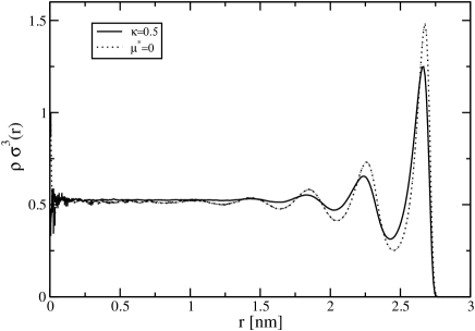
Figure 1: Density profiles $\rho(r)$ as functions of the radial distance $r$ for a system with $N=1000$ and $R=3$ nm ($\rho^{*}=0.53$). The solid curve is for dipoles ($\mu^{*}=2$) with $\kappa=0.5$. The different values of $\kappa$ coincide on this scale. The dotted curve is the reference for particles without dipoles ($\mu^{*}=0$).

Profiles obtained for a cavity of radius $R=3$ nm, $N=1000$, $\mu^{*}=2$ and four values of $\kappa$ are compared in Fig. 1 to the profile corresponding to non-polar molecules ($\mu^{*}=0$) under otherwise identical conditions. All profiles exhibit the expected layering near the confining spherical surface Senapati and Chandra (1999). As expected the layering effect is even more pronounced for the smaller cavity radius $R=2.5$ nm which we also explored (data not shown). There are two striking results: the profiles observed for the four different values of $\kappa$ are nearly indistinguishable, i.e. the radial structure turns out to be practically independent of the polarisability of the confining continuum. However the profile $\rho(r)$ changes substantially when $\mu^{*}$ is set equal to zero, i.e. in the absence of any electrostatic coupling between molecules and with the embedding medium: the layering is seen in Fig. 1 to be considerably enhanced, and to extend deeper towards the centre of the cavity.

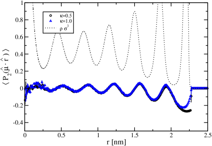
Figure 2: The order parameter $\langle P_{2}(\hat{\mu}\cdot\hat{r})\rangle$ as a function of the distance to the centre of the cavity ($N=1000$, $R=2.5$ nm). The dotted curve shows the corresponding density profile $\rho^{*}(r)$ for $\kappa=0.5$.

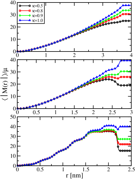
Figure 3: The average absolute value $\langle|\vec{M}(r)|\rangle$ of the total dipole moment of all dipoles within a distance $r$ from the centre of the cavity, for the various values of $\kappa$. From top to bottom cavities of size $R=4$, 3, and 2.5 nm.

These findings are qualitatively confirmed in the cases of the larger ($R=4$ nm) and smaller ($R=2.5$ nm) cavities. The conclusion to be drawn here is that the dipolar interactions between molecules tend to smooth out the layering imposed by the short-range, excluded volume effects. The orientations of individual dipoles relative to the normal to the surface are characterised by the local order parameters $\langle P_{1}(\hat{\mu}\cdot\hat{r})\rangle_{r}$ and $\langle P_{2}(\hat{\mu}\cdot\hat{r})\rangle_{r}$, where $P_{l}$ denotes the $l$th order Legendre polynomial, $\hat{r}$ and $\hat{u}$ are the unit vectors along the radial vector $\vec{r}$ and the dipole moment $\vec{\mu}$, and the statistical average is taken over dipole configurations within spherical shells of radius $r$ and width $\delta$. Because of the $\vec{\mu}_{i}\rightarrow-\vec{\mu}_{i}$ inversion symmetry, $\langle P_{1}(\hat{\mu}\cdot\hat{r})\rangle_{r}$ is identically zero, while $\langle P_{2}(\hat{\mu}\cdot\hat{r})\rangle_{r}$ is plotted in Fig. 2 as a function of $r$ for several values of $\kappa$. $\langle P_{2}(\hat{\mu}\cdot\hat{r})\rangle_{r}$ is seen to depend very little on $\kappa$, except very close to the outer surface. The order parameter oscillates somewhat out of phase with the oscillations in the density profile shown in a frame of the same figure. Near the maxima of the latter, which correspond to well defined shells of polar molecules, the order parameter is predominantly negative, signalling a preferential orientation of the dipoles orthogonal to the radial vector $\hat{r}$, i.e. the dipoles orient preferentially parallel to the confining surface, irrespective of the embedding medium, suggesting a vortex-like pattern of the confined dipoles.

Qualitatively similar behaviour is observed for the larger cavities (lower overall densities), except that, as expected, the oscillations in $\langle P_{2}(\hat{\mu}\cdot\hat{r})\rangle_{r}$ are less pronounced. The preferential alignment of dipoles parallel to the confining surface was also observed in earlier work Zhang et al. (1995).

Consider next the total dipole moment $\vec{M}(r)$ within a sphere of radius $r\leq R$. While $\langle\vec{M}(r)\rangle$ vanishes again by symmetry, the statistical average of the absolute value of $\vec{M}(r)$ shows an interesting behaviour, illustrated in Fig. 3 for the three different pore radii $R$ under investigation. For the two lower densities $\langle|\vec{M}(r)|\rangle$ is seen to increase roughly as $N_{r}^{1/2}$ i.e. $r^{3/2}$, up to $r\simeq R/2$, as one would expect if the $N_{r}$ dipole moments within a sphere of radius $r$ were uncorrelated. This part of the curve is essentially independent of $\kappa$.

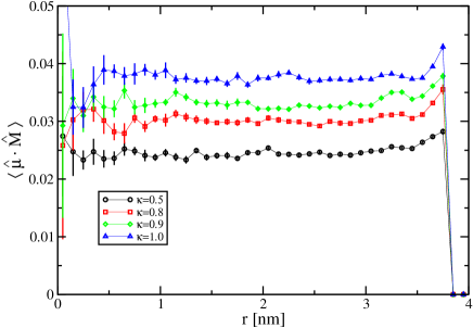
Figure 4: The correlation $\langle\hat{\mu}\cdot\hat{M}\rangle$ of the individual dipoles with the direction of the total dipole moment of all particles in the cavity as a function of the distance $r$ from the centre for a $R=4$ nm cavity, and $0.5\leq\kappa\leq 1$.

Beyond $r\simeq R/2$ the four curves diverge and show some structure for the smaller cavities ($R=3$ and 2.5 nm). For a given $r$, the value of $\langle|\vec{M}(r)|\rangle$ increases with increasing $\kappa$, reflecting an enhanced effect of the image dipoles as $\epsilon^{\prime}$ increases (See. Eq. 3). Although not evident in the density profiles of Fig. 1, the effect of the polarisation of the confining medium is seen to have a very significant effect on the dipolar properties of the confined system. This is also evident in Fig. 4 where we plot the average of the projection of the dipole moments of the individual dipoles within a shell of radius $r$ and small thickness along the total dipole moment $\vec{M}$ of the sample, $\langle\hat{\mu}\cdot\hat{M}\rangle$. The projection is small, but positive signalling that the individual dipoles tend to align along the overall dipole moment. Moreover, it is quasi-independent of the distance $r$, and increases with $\kappa$, i.e. as one moves from vacuum outside the cavity, to a metallic confining medium.

We finally turn to the static dielectric permittivity profile of the confined fluid. This can be related to the dipolar fluctuations by linear response theory Ballenegger and Hansen (2005), or by measuring the total polarisation induced in the sample by the “external” electric field due to a charge placed at the origin of the cavity. Let $\vec{m}(r)$ denote the microscopic polarisation density:

$$\vec{m}(r)=\sum_{i=1}^{N}\vec{\mu}_{i}\delta(\vec{r}-\vec{r}_{i})$$ (8)

The overall dipole moment of the sample is then:

$$\vec{M}=\int_{{\cal D}_{\text{cavity}}}d\vec{r}\vec{m}(r)$$ (9)

where the integration is over the whole volume of the cavity. The linear response result for the permittivity profile $\epsilon(r)$ is given by the following generalisation Ballenegger and Hansen (2005) of Kirkwood’s classical results for the bulk Kirkwood (1939):

$$\frac{(\epsilon(r)-1)(2\epsilon^{\prime}+1)}{2\epsilon^{\prime}+\epsilon(r)}=\frac{4\pi\beta}{3}\left[\langle\vec{m}(r)\cdot\vec{M}\rangle-\langle\vec{m}(r)\rangle\cdot\langle\vec{M}\rangle\right]$$ (10)

Far from the confining surface bulk behaviour may be expected, and replacing $\vec{m}$ by $\vec{M}/V$, one recovers Kirkwood’s formula. Near the surface rotational invariance is broken and the permittivity becomes a tensor with longitudinal (i.e. parallel to $\vec{r}$) and transverse components.

Note that equation (10) is exact provided that there exists a local relationship between the polarisation and the internal (Maxwell) electric field. It defines a permittivity profile $\epsilon(r)$ which may be expected to go to a constant “bulk” value far from the confining surface, as will be confirmed by our simulation data, at least at low or moderate densities. An approximate method for estimating such “bulk” values within cavities has been put forward by Berendsen Berendsen (1972); Adams and McDonald (1995), but the limitations of this method have been illustrated in Ref.Ballenegger and Hansen (2005).

In MD simulations, the correlation function on the right hand side of the Eq. (10) is estimated by averaging over all dipole moments of particles within a spherical shell of radius $r$ and width $\simeq\sigma$. In the “external field” method, an additional particle is placed at the origin, with the (extended) dipole replaced by a simple proton charge $e$ at its centre. If one assumes a local relationship between the radial polarisation density $P(r)=\langle\hat{r}\cdot\vec{m}(\vec{r})\rangle$ and the local radial electric field $E(r)=\hat{r}\cdot\vec{E}(\vec{r})$ of the form:

$$P(r)=\epsilon_{0}\chi(r)E(r)=[\epsilon(r)-1]E(r)$$ (11)

then, $\epsilon(r)$ follows from elementary electrostatics Ballenegger and Hansen (2005). Let $Q(r)=e+Q_{\text{ind}}(r)$ be the total charge contained inside a sphere of radius $r$, which is easily estimated from the MD simulations for the extended dipole model. As a consequence of the divergence theorem, $Q_{\text{ind}}(r)$ inside the sphere of radius $r$ is related to the polarisation density by:

$$P(r)=-\frac{Q_{\text{ind}}(r)}{4\pi r^{2}}$$ (12)

while the electric field $E(r)$ is related to $Q(r)$ by:

$$E(r)=\frac{Q(r)}{r^{2}}$$ (13)

Substitution of (12) and (13) in Eq. (11) leads to the desired estimate:

$$\epsilon(r)=\frac{e}{e-4\pi r^{2}P(r)}=\frac{1}{1+Q_{\text{ind}}(r)/e}$$ (14)

The presence of the central charge introduces some distortion of the density profiles near the centre of the cavity, as illustrated in Fig. 5. An excluded volume zone and subsequent layering now appear at small $r$, but the profiles are virtually unchanged for $r\gtrsim R/2$ relative to the case without central charge. Note that adding the additional particle changes the overall density inside the cavity by only one part in 1000, so that a comparison between fluctuation and response results remains meaningful.

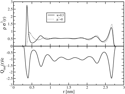
Figure 5: The radial density profiles $\rho(r)$ in the presence of a charge at the centre of the cavity for $\kappa=0.5$ ($R=3$ nm, $\mu^{*}=2$). The different values of $kappa$ coincide on this scale. The dotted curve is the reference profile for particles without dipole. In the lower part of the figure the corresponding charge distribution $Q_{\text{ind}}(r)/e$ is shown.

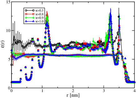
Figure 6: $\epsilon(r)$ versus the distance $r$ obtained from the fluctuation formula (10) (open symbols) and from the response to a central charge (14) (filled symbols) for $\mu^{*}=2$, $R=4$nm, and $0.5\leq\kappa\leq 1$.

Plots of the induced charge $Q_{\text{ind}}(r)$ inside a sphere of radius $r$ are shown as a function of $r$ in Fig. 5 for the cavity with radius $R=3$ nm. $Q_{\text{ind}}(r)$ “overscreens” the external charge $e$ at the centre, at short distances, before oscillating around a negative value and going to zero as $r\rightarrow R$ . At the lower overall density ($R=4$ nm), $Q_{\text{ind}}(r)$ stabilises around a “bulk” value above $-e$ at intermediate distances (data not shown), while no such “bulk” regime is observed at higher density ($R=3$ nm) . Remarkably $Q(r)$ is practically independent of $\epsilon^{\prime}$ (or $\kappa$).

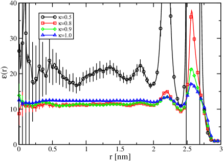
Figure 7: $\epsilon(r)$ versus the distance $r$ obtained from the fluctuation formula (10) for $\mu^{*}=2$, $R=3$ nm, and $0.5\leq\kappa\leq 1$.

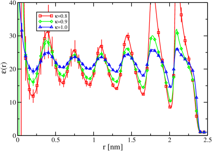
Figure 8: $\epsilon(r)$ versus the distance $r$ obtained from the fluctuation formula (10)for $\mu^{*}=2$, $R=2.5$ nm, and $\kappa=0.8$, 0.9, and 1.

The values of $\epsilon(r)$ derived from Eq. (14) are compared to the corresponding values estimated from the fluctuation formula (10) in Fig. 6 for the lower density ($R=4$ nm), $\mu^{*}=2$ and four values of $\kappa$. Clearly Eq. (14) can only yield physically acceptable results as long as $Q_{\text{ind}}(r)/e>-1$. At small and large $r$ the oscillations in $Q(r)$ lead to unphysical values of $\epsilon(r)$, signalling the break-down of the local assumption (11), as already noted in Ref. Ballenegger and Hansen (2005) for the special case $\kappa=0.5$ ($\epsilon^{\prime}=1$). In that case the data shown in Fig. 6 point, however, to two surprising findings. First of all $\epsilon(r)$ profiles derived from Eq. (14) appear to be independent of $\kappa$, due to the quasi-independence of $Q_{\text{ind}}(r)$ on $\kappa$ in Fig. 5. On the other hand the $\epsilon(r)$ values derived from the fluctuation formula (10) for $\epsilon^{\prime}>1$ ($\kappa=0.8$, 0.9, and 1) are practically independent of $\kappa$, but lie significantly below the results for $\kappa=0.5$. In other words, the polarisation of the surrounding medium leads to a reduction of the permittivity of the sample inside the cavity. However the response to a central charge $e$ appears to be significantly non-linear, but independent of $\kappa$. It would be very difficult to measure the response to a smaller external charge at the cavity centre, due to an unfavourable signal to noise ratio.

$R$	$\rho^{*}$	$\kappa$	$\epsilon_{b}$	$\epsilon(\omega=0)$
4 nm	0.23	0.5	7.6	4.8
		0.8	5.7	4.5
		0.9	5.6	4.6
		1.0	5.7	4.8
3 nm	0.53	0.5	19.7	10.5
		0.8	11.3	9.0
		0.9	11.3	9.5
		1.0	12.3	10.7
2.5 nm	0.92	0.5		18.2
		0.8	20.8	13.6
		0.9	20.8	15.1
		1.0	21.8	18.4

Table 3: The estimated “bulk” permittivity $\epsilon_{b}$ and zero-frequency permittivity $\epsilon(\omega=0)$ values for the different cavity sizes $R$, reduced densities $\rho^{*}$, and $\kappa$.

Results for the smaller cavity ($R=3$ nm), i.e. higher overall density are shown in Fig. 7. As is already clear from Fig. 5, Eq. (14) is no longer applicable, because the strong oscillations in $Q_{\text{ind}}(r)$ go repeatedly through the value $-e$ and a “bulk”-like regime is never reached. Hence only the results from the fluctuation formula (10) are shown. The behaviour as a function of $\kappa$ qualitatively confirms one of the observations already made at the lower density ($R=4$ nm) shown in Fig.6, namely that the “bulk” values of $\epsilon$ agree within statistical errors for $\epsilon^{\prime}>1$ ($\kappa=0.8$, 0.9, and 1), but are roughly a factor 2 lower than the value measured for $\epsilon^{\prime}=1$. The error bars on the latter are much larger than those associated with the data for the polarisable embedding medium.

At the highest density ($R=2.5$ nm), $\epsilon(r)$ oscillates roughly in phase with the density oscillations. A proper “bulk” regime is never reached for the $N=1000$ particle system, but one can extract a rough value of $\epsilon_{b}$ around which $\epsilon(r)$ oscillates. These values, given in Table 3, depend only weakly on $\kappa$, except for $\kappa=0.5$ (vacuum outside the cavity), when $\epsilon_{b}$ is roughly a factor of two larger than for $\kappa>0.5$; the very noisy permittivity profile for $\kappa=0.5$ is not shown in Fig. 8. The best estimates of $\epsilon_{b}$ as a function of cavity radius $R$ and of $\kappa$ are listed in Table 3. The permittivity of the confined fluid is strongly reduced compared to its value in a uniform (bulk) fluid at the same density and temperature.

IV Relaxation

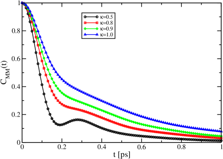
Figure 9: The total dipole autocorrelation function $C_{MM}(t)$ versus time for $R=4$ nm, $\mu^{*}=2$, $0.5\leq\kappa\leq 1$.

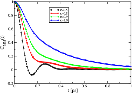
Figure 10: The total dipole autocorrelation function $C_{MM}(t)$ versus time for $R=3$ nm, $\mu^{*}=2$, $0.5\leq\kappa\leq 1$.

The dielectric response of a polar sample is characterised by the frequency-dependent complex dielectric permittivity $\epsilon(\omega)=\epsilon_{1}(\omega)+\imath\epsilon_{2}(\omega)$. Within the linear response regime the latter is determined by the Laplace transform of the dynamical response function $\Phi_{MM}(t)$ which relates the induced total dipole moment of the sample to a time-dependent external field Madden and Kivelson (1984); Hansen and McDonald (2006):

$$\langle\Delta\vec{M}(t)\rangle=\int_{-\infty}^{t}\Phi_{MM}(t-t^{\prime})\vec{E}_{\text{ext}}(t^{\prime})dt^{\prime}$$ (15)

where $\Phi_{MM}$ is a scalar for a spherical sample. According to the standard rules of linear response Hansen and McDonald (2006):

$$\begin{split}\Phi_{MM}(t)&=-\beta\langle\dot{\vec{M}}(t)\cdot\vec{M}(0)\rangle\\ &=-\beta\dot{C}_{MM}(t)\langle M^{2}\rangle\end{split}$$ (16)

where the dot denotes a time derivative and $C_{MM}(t)$ is the normalised total dipole moment correlation function of the unperturbed sample:

$$C_{MM}(t)=\frac{\langle\vec{M}(t)\cdot\vec{M}(0)\rangle}{\langle M^{2}\rangle}$$ (17)

The complex susceptibility is:

$$\tilde{\chi}_{MM}(z)=\int_{0}^{\infty}\Phi_{MM}(t)e^{\imath zt}dt$$ (18)

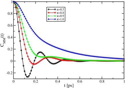
Figure 11: The total dipole autocorrelation function $C_{MM}(t)$ versus time for $R=2.5$ nm, $\mu^{*}=2$, $0.5\leq\kappa\leq 1$.

where $z=\omega+\imath\varepsilon$, and:

$$\lim_{\varepsilon\rightarrow 0^{+}}\tilde{\chi}_{MM}(z)=\chi_{1}(\omega)+\imath\chi_{2}(\omega)$$ (19)

According to the fluctuation-dissipation theorem, a direct consequence of Eq. (16):

$$\tilde{\chi}_{MM}(z)=\beta\langle M^{2}\rangle\left[C_{MM}(t=0)+\imath z\tilde{C}_{MM}(z)\right]$$ (20)

This implies that the spectrum of the correlation function $C_{MM}(t)$ is related to the imaginary part of the susceptibility

$$\begin{split}\hat{C}_{MM}(\omega)&=\frac{1}{2\pi}\int_{-\infty}^{\infty}e^{\imath\omega t}C_{MM}(t)dt\\ &=\frac{k_{B}T}{\pi\omega}\frac{\chi_{2}(\omega)}{\langle M^{2}\rangle}\end{split}$$ (21)

Finally, for the system under consideration, i.e. a polar fluid confined to a spherical cavity surrounded by a dielectric continuum of permittivity $\epsilon^{\prime}$, the frequency-dependent permittivity of the sample is related to the complex susceptibility by Titulaer and Deutch (1974) :

$$\begin{split}\frac{\epsilon(\omega)-1}{\epsilon-1}\frac{2\epsilon^{\prime}+\epsilon}{2\epsilon^{\prime}+\epsilon(\omega)}&=\frac{k_{B}T}{\langle M^{2}\rangle}\tilde{\chi}_{MM}(\omega)\\ &=\frac{k_{B}T}{\langle M^{2}\rangle}\left[\chi_{1}(\omega)+\imath\chi_{2}(\omega)\right]\end{split}$$ (22)

where $\epsilon\equiv\epsilon(\omega=0)$ is the static permittivity of the sample.

The static permittivity $\epsilon$ is given by the $\omega\rightarrow 0$ limit of Eq. (22) which results in:

$$\frac{(\epsilon-1)(2\epsilon^{\prime}+1)}{2\epsilon^{\prime}+\epsilon}=\frac{4\pi\beta}{3}\frac{\langle M^{2}\rangle}{V}$$ (23)

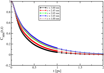
Figure 12: The dipole autocorrelation function $C_{MM}(r,t)$ versus time for $R=3$ nm, $\mu^{*}=2$, $\kappa=1$ and several values of $r$.

Thus $\epsilon(\omega=0)$ is determined by the fluctuation of the total dipole moment $\vec{M}$ of the spherical sample. The result differs from the “bulk” value $\epsilon_{b}$ determined as explained in Sect. III, from the profile $\epsilon(r)$ calculated from Eq. (10). It characterises the global response of the polar fluid trapped in the cavity rather than the local response, away from the confining surface. The values of $\epsilon$ are seen to lie systematically below those of $\epsilon_{b}$, particularly so in the case $\kappa=0.5$.

Hence all information required to compute $\epsilon(\omega)$ is contained in the total dipole autocorrelation function (17). MD results for $C_{MM}(t)$ are shown in Figures 9 – 11 for the three cavity radii $R=4$, 3, and 2.5 nm, and four values of $\kappa$. The correlation functions are seen to relax to zero over a time scale of about 1 ps, which is an order of magnitude shorter than the relaxation time observed in the bulk for the same model Ballenegger and Hansen (2004). The most striking feature is the strong sensitivity of $C_{MM}(t)$ to the polarisability of the confining medium, i.e. to $\kappa$. For all three radii, the relaxation is slowest for $\kappa=1$ (metallic boundary), and becomes faster as $\kappa$ decreases. Marked oscillations appear when $\kappa=0.5$ ($\epsilon^{\prime}=1$) particularly so at the highest density ($R=2.5$ nm). Simulations carried out on smaller samples of $N=250$ dipoles show that the relaxation patterns appear to be independent of the sample size characterised by $R$ and $N$, provided the reduced overall density $\rho^{*}=\rho\sigma^{3}$ is the same. The decrease of the relaxation time of $C_{MM}(t)$ with $\kappa$ agrees with the behaviour predicted for a Debye dielectric Neumann and Steinhauser (1983). There is no obvious explanation for the oscillation observed for $\kappa=0.5$. These oscillations are indicative of collective behaviour reminiscent of the dipolaron mode observed in MD simulations of longitudinal dipolar fluctuations at finite wavenumber in bulk model polar fluids Pollock and Alder (1981).In an effort to gain a better understanding of the dipolar relaxation, we have also computed the normalised correlation functions:

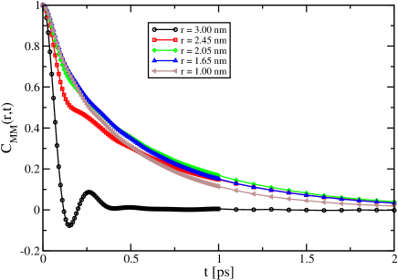
Figure 13: The dipole autocorrelation function $C_{MM}(r,t)$ versus time for $R=3$ nm, $\mu^{*}=2$, $\kappa=0.5$ and several values of $r$.

$$C_{MM}(r,t)=\frac{\langle\vec{M}(r,t)\cdot\vec{M}(r,0)\rangle}{\langle|\vec{M}(r)|^{2}\rangle}$$ (24)

where $\vec{M}(r,t)$ is the instantaneous total dipole moment of all the molecules contained inside a sphere of radius $r\leq R$. The MD data are shown in Figures 12 and 13 for $\kappa=1$ and $\kappa=0.5$ respectively. In the former (metallic boundary) case $C_{MM}(r,t)$ changes only moderately with $r$. This is not totally unexpected, since the “bulk” permittivity of the sample is relatively large under these conditions ($\epsilon\simeq 12$), as seen from Fig. 7, and hence the dielectric discontinuity is not too strong relative to the metallic embedding medium. The situation is very different when $\kappa=0.5$ (Fig. 13). In this case $C_{MM}(r,t)$ changes relatively little with $r$, and decays monotonically except when $r=R$ (corresponding to the autocorrelation function of the total dipole moment of the sample), when $C_{MM}$ decays much faster and oscillates. Thus the dynamics of the molecular dipole moments inside the outer shell, in direct contact with the surface separating the confined fluid from vacuum, has a dramatic effect on the total dipole correlation function.

Real and imaginary parts of the complex susceptibility (19) are plotted in Fig. 14 for the cavity of radius $R=3$ nm, and 4 values of $\kappa$. $\chi_{1}(\omega)$ and $\chi_{2}(\omega)$ vary with $\omega$ in a manner reminiscent of bulk behaviour Pollock and Alder (1981). However they are rather sensitive to $\kappa$, i.e. to the permittivity of the surrounding medium. On the contrary the real and imaginary parts of the frequency-dependent permittivity defined by Eq. (22), are remarkably insensitive to $\kappa$, except for $\epsilon_{1}(\omega)$ in the static ($\omega\rightarrow 0$) limit, as illustrated in Fig. 15. This insensitivity to $\kappa$ reflects the fact that, contrary to $\tilde{\chi}_{MM}(\omega)$, $\epsilon(\omega)$ measures the response of the polar fluid to the local, internal field.

The resulting Cole–Cole plots, shown in Fig. 16, differ strongly from the semi-circular shape of the simple Debye theory, as one might expect. The high-frequency part is very insensitive to $\kappa$, while the differences in the low-frequency range reflect the significant differences in static values of $\epsilon$.

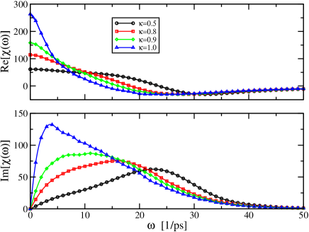
Figure 14: The real and imaginary part of the complex susceptibility as a function of the frequency $\omega$ ($R=3$nm).

V Conclusion

We have reported the first systematic attempt to investigate the dependence of the structure, static and dynamic correlations and response of a drop of polar fluid confined to a spherical cavity, on the permittivity $\epsilon^{\prime}$ of the embedding medium. The work extends earlier investigations which were restricted to the case of a non-polarisable external medium ($\epsilon^{\prime}=1$) Senapati and Chandra (1999); Ballenegger and Hansen (2005) by treating the interactions between the charge distribution associated with the extended dipoles of the trapped fluid, and the image charges in an approximate, but accurate way, which provides an efficient alternative to the more cumbersome variational method proposed elsewhere Allen et al. (2001). The present treatment of electrostatic boundary conditions for the electric field of individual charges within the confined sample does not rely on macroscopic reaction field considerations, but is restricted to the spherical geometry.

The MD simulations were run for samples of $N=1000$ polar molecules confined to cavities of radii $R=4$, 3, and 2.5 nm, which amount to effective densities of $\rho^{*}=0.23$, 0.53, and 0.92. Some test runs were carried out for a smaller sample of $N=250$ molecules, and no significant $N$-dependence was observed. The larger $N=1000$ particle system allows a “bulk” regime to be reached within a substantial fraction of the accessible volume (say up to $r\simeq R/2$), except for the smallest cavity (i.e. highest effective density $\rho^{*}=0.92$). All calculations were made with a reduced extended dipole moment $\mu^{*}=2$, comparable to that of water.

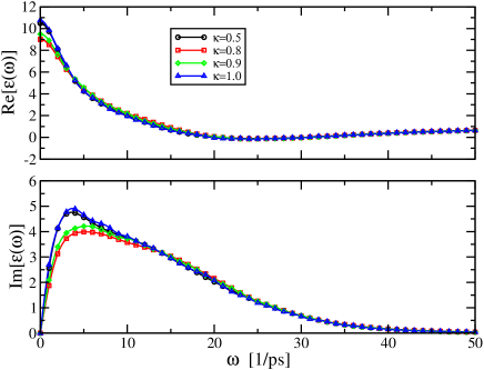
Figure 15: The real and imaginary part of the complex permittivity as a function of the frequency $\omega$ ($R=3$nm).

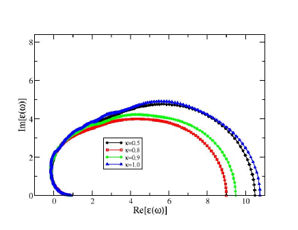
Figure 16: Cole–Cole plot: imaginary versus real part of the permittivity ($R=3$nm).

The main conclusions to be drawn from our MD data may be summarised as follows:

1. The structural properties embodied in the density profiles $\rho(r)$ and the order parameter profiles $\langle P_{2}(\hat{\mu}\cdot\hat{r})\rangle$ are remarkably insensitive to the embedding medium, i.e. to $\kappa$. The density profiles show significantly less structure than their $\mu=0$ counterparts. The order parameter profiles point to a preferential alignment of the dipoles parallel to the confining surface, as already reported in earlier studies of related systems Senapati and Chandra (1999); Zhang et al. (1995).

2. The static permittivity profiles $\epsilon(r)$ may be calculated from the generalised Kirkwood fluctuation relation (10)Ballenegger and Hansen (2005), or by measuring the polarisation profile $P(r)$, or charge profile $Q(r)$ induced by an “external” charge placed at the centre of the spherical cavity (cf. Eq. (14)). The latter method can only be implemented at the lowest density ($R=4$ nm) and points to a significant non-linearity compared to the predictions of the fluctuation formula, when the “external” charge is the proton charge. The fluctuation formula yields oscillatory $\epsilon(r)$ profiles which essentially reflect the oscillations in the density profiles $\rho(r)$. At the two lower densities ($R=4$ and 3 nm) the oscillations are sufficiently damped away from the confining surface for a “bulk” regime to be reached inside the cavity allowing the definition of a “bulk” permittivity $\epsilon_{b}$. The latter turns out to be relatively insensitive to $\kappa$, except for $\kappa=0.5$ (cavity surrounded by vacuum), which leads to substantially larger values of $\epsilon_{b}$. At the highest density ($R=2.5$ nm), the oscillations of $\epsilon(r)$ extend up to the centre , so that no proper “bulk” regime is reached . A rough estimate of $\epsilon_{b}$ may be extracted by averaging over oscillations. In all cases the “bulk” permittivity inside the cavity is strongly reduced relative to the values expected for a uniform (genuinely bulk) fluid under comparable conditions, an observation also made in earlier work Senapati and Chandra (1999); Zhang et al. (1995).

3. While the static properties of a confined drop of polar fluid turn out the be surprisingly insensitive to the permittivity of the external medium except when $\epsilon^{\prime}\rightarrow 1$, the dynamical properties depend much more on $\epsilon^{\prime}$ (or equivalently $\kappa$). The most striking illustration is the correlation function $C_{MM}(t)$ of the total dipole moment of the sample, which relaxes faster when $\kappa\simeq 0.5$ (cf. Figs. 9 – 11). As also noted in earlier work Zhang et al. (1995) on confined water, the relaxation of $C_{MM}(t)$ is much faster than under comparable bulk conditions Ballenegger and Hansen (2004). While such a behaviour may be rationalised by the absence of long-range dipolar interactions with distant molecules in the case of the confined system, which may lead to a lower collective “inertia” compared to the bulk, a detailed theoretical interpretation of the observation is still lacking.

4. The complex, dynamical permittivity was estimated from Eq. (22) The corresponding Cole–Cole plots differ considerably from the semi-circular shape associated with exponential Debye relaxation, as was to be expected from the complex relaxation pattern of the $C_{MM}(t)$ correlation function. While the high frequency regions of the real and imaginary parts of the permittivity are quite insensitive to the value of $\kappa$, significant deviations occur in the low-frequency regime (cf. Figs. 14 and 15) which are reflected in the right-hand parts of the Cole–Cole plots in Fig. 16. The zero-frequency limits $\epsilon=\epsilon(\omega=0)$ of the dynamical permittivity differ substantially from the “bulk” limits $\epsilon_{b}$ of the static permittivity profiles $\epsilon(r)$, as shown in Table 3, which is not surprising since $\epsilon$ and $\epsilon_{b}$ measure “global” and “local” responses respectively.

A theoretical analysis of the dynamical properties of confined polar fluids is left for future work. We also plan to explore the static and dynamic properties of polar fluids in narrow pores (one-dimensional confinement) and in slits (two-dimensional confinement).

Appendix A

In this appendix we derive the electrostatic potential inside a spherical cavity of radius $R$ and permittivity $\epsilon$, which results from the polarisation of an infinite medium with permittivity $\epsilon^{\prime}$ surrounding the cavity due to an internal charge distribution.

The electrostatic potential at $\vec{r}$, due to a single charge $Q$ at position $\vec{d}$ inside the cavity, can be formally expanded in Legendre Polynomials $P_{l}$ as:

$$\begin{split}\Phi^{\text{in}}&=\frac{Q}{4\pi\epsilon}\frac{1}{|\vec{r}-\vec{d}|}+\sum_{l=0}^{\infty}A_{l}r^{l}P_{l}(\cos\theta);~{}~{}~{}r<R\\ \Phi^{\text{out}}&=\sum_{l=0}^{\infty}\frac{B_{l}}{r^{l+1}}P_{l}(\cos\theta);~{}~{}~{}~{}~{}~{}~{}~{}~{}~{}~{}~{}~{}~{}~{}~{}~{}~{}~{}~{}~{}r>R\end{split}$$ (25)

where $\cos\theta=\hat{r}\cdot\hat{d}$, and the expansion coefficients $A_{l}$ and $B_{l}$ follow from the boundary conditions of a continuous tangential and a discontinuous normal electric field at the border of the cavity $r=R$:

$$\begin{split}\frac{\partial\Phi^{\text{in}}}{\partial\theta}&=\frac{\partial\Phi^{\text{out}}}{\partial\theta}\\ \epsilon\frac{\partial\Phi^{\text{in}}}{\partial r}&=\epsilon^{\prime}\frac{\partial\Phi^{\text{out}}}{\partial r}\end{split}$$ (26)

By expanding the direct term $1/|\vec{r}-\vec{d}|$ of the internal electrostatic field $\Phi^{\text{in}}$ at the cavity wall in Legendre polynomials, solving these boundary conditions is straightforward and one finds:

$$\begin{split}\Phi^{\text{in}}&=\frac{Q}{4\pi\epsilon}\left[\frac{1}{|\vec{r}-\vec{d}|}+(1-2\kappa)\sum_{l}\frac{l+1}{l+\kappa}\frac{d^{l}r^{l}}{R^{2l+1}}P_{l}(\cos\theta)\right]\\ \Phi^{\text{out}}&=\frac{Q\kappa}{4\pi\epsilon^{\prime}}\sum_{l}\frac{2l+1}{l+\kappa}\frac{d^{l}}{r^{l+1}}P_{l}(\cos\theta)\end{split}$$ (27)

where we introduced $\kappa\equiv\epsilon^{\prime}/(\epsilon+\epsilon^{\prime})$. This result can be simplified by rewriting the fraction appearing inside the summations:

$$\begin{split}\Phi^{\text{in}}=&\frac{Q}{4\pi\epsilon}\left[\frac{1}{|\vec{r}-\vec{d}|}+(1-2\kappa)\sum_{l}\frac{d^{l}r^{l}}{R^{2l+1}}P_{l}(\cos\theta)+\right.\\ &\left.\frac{(1-2\kappa)(1-\kappa)}{\kappa R}\sum_{l}\frac{\kappa}{l+\kappa}\frac{d^{l}r^{l}}{R^{2l}}P_{l}(\cos\theta)\right]\end{split}$$ (28)

$$\begin{split}\Phi^{\text{out}}=&\frac{Q\kappa}{4\pi\epsilon^{\prime}}\left[2\sum_{l}\frac{d^{l}}{r^{l+1}}P_{l}(\cos\theta)+\right.\\ &\left.\frac{1-2\kappa}{\kappa r}\sum_{l}\frac{\kappa}{l+\kappa}\frac{d^{l}}{r^{l}}P_{l}(\cos\theta)\right]\end{split}$$ (29)

In both cases the first summation represents the expansion in Legendre polynomials of an inverse distance. In the latter this is the distance $|\vec{r}-\vec{d}|$ to the original charge. In the former, however, this is the distance to a location $\vec{D}\equiv=(R/d)^{2}\vec{d}$ outside the cavity. The second summation can be simplified by expanding the Legendre polynomial in terms of $\exp(\imath n\theta)$ (See Ref. Gradshteyn and Ryzhik (2000), Eq.[8.911.4]). This results in:

$$\begin{split}\Phi^{\text{in}}=&\frac{1}{4\pi\epsilon}\left[\frac{Q}{|\vec{r}-\vec{d}|}+(1-2\kappa)\frac{Q(R/d)}{|\vec{r}-\vec{D}|}\right]+\\ &\frac{Q(1-2\kappa)}{4\pi\epsilon^{\prime}R}F_{1}(\kappa,\frac{1}{2},\frac{1}{2},1+\kappa;xe^{\imath\theta},xe^{-\imath\theta})\end{split}$$ (30)

$$\begin{split}\Phi^{\text{out}}=&\frac{1}{4\pi\epsilon^{\prime}}\frac{2\kappa Q}{|\vec{r}-\vec{d}|}+\\ &\frac{Q(1-2\kappa)}{4\pi\epsilon^{\prime}r}F_{1}(\kappa,\frac{1}{2},\frac{1}{2},1+\kappa;ye^{\imath\theta},ye^{-\imath\theta})\end{split}$$ (31)

where we introduced $x\equiv r/D$ and $y\equiv d/r$, while $F_{1}$ is a hyper-geometric function in two variables (See Ref. Gradshteyn and Ryzhik (2000), Eq.[9.180.1]). Note that the location $\vec{D}$ corresponds to the position where a single image charge should be placed in the case of metallic boundary conditions Jackson (1999).

Although one can in principle calculate or tabulate the hyper-geometric function, one can show that in the present case of a confined dipolar fluid this term can safely be neglected. In doing so, we approximate the induced electrostatic potential field by a single external image charge. Note that this approximation is exact in the case of a vacuum outside ($\kappa=1/2$) and in the case of metallic boundary conditions ($\epsilon^{\prime}\rightarrow\infty$).

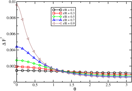
Figure 17: The absolute error in the reduced force $\Delta F^{*}$ of the force of a unit charge at a distance $d/R=0.9$ from the origin on a unit charge at a position $(r,\theta)$ inside a cavity with radius $R=2.5$ nm and $\kappa=0.8$.

There are two intuitive arguments for making this approximation. Firstly, the field, except near the cavity wall, is mainly determined by the local charge distribution inside the cavity, rather than the image charge distribution arising from the polarisation. The second reason is that, since we consider a fluid of extended dipoles where the charge separation is roughly a third of the particle diameter, the two neglected parts of the induced charge distribution of both charges that form a dipole will cancel to a large extent.

In order to illustrate that the error made by the approximation is indeed small, we place a unit charge at a distance $d/R=0.9$ from the origin in a cavity of radius $R=2.5$ nm and $\kappa=0.8$, and measure the reduced force $F^{*}$ in terms of the force between two unit charges at a distance $\sigma$. A second charge is put at various distances $r/R$ from the origin of the cavity, the result of which is shown in Fig. 17. The error increases both with decreasing cavity radius, and on approaching the cavity wall with one or both charges. Note, that although the absolute error increases also when the charges get closer, the relative error in that case decreases due to the singular behaviour of the direct interaction between the charges.

References

- Debye (1929) P. Debye, Polar Molecules (Dover, New York, 1929).
- Kirkwood (1939) J. G. Kirkwood, J. Chem. Phys. 7, 911 (1939).
- Onsager (1936) L. Onsager, J. Am. Chem. Soc. 58, 1486 (1936).
- Madden and Kivelson (1984) P. A. Madden and D. Kivelson, Adv. Chem. Phys. 56, 467 (1984).
- Weis and Levesque (2005) J. J. Weis and D. Levesque, Adv. Polym. Sci. 185, 163 (2005).
- Neumann (1983) M. Neumann, Mol. Phys. 50, 841 (1983).
- Neumann and Steinhauser (1983) M. Neumann and O. Steinhauser, Chem. Phys. Lett. 102, 508 (1983).
- Senapati and Chandra (1999) S. Senapati and A. Chandra, J. Chem. Phys. 111, 1223 (1999).
- Teschke et al. (2001) O. Teschke, G. Ceotto, and E. F. de Souza, Phys. Rev. E 64, 011605 (2001).
- Stern and Feller (2003) H. A. Stern and S. E. Feller, J. Chem. Phys. 118, 3401 (2003).
- Ballenegger and Hansen (2003) V. Ballenegger and J.-P. Hansen, Europhys. Lett. 63, 381 (2003).
- Ballenegger and Hansen (2005) V. Ballenegger and J.-P. Hansen, J. Chem. Phys. 122, 114711 (2005).
- Bagchi and Chandra (1991) B. Bagchi and A. Chandra, Adv. Chem. Phys. 80, 1 (1991).
- Ballenegger and Hansen (2004) V. Ballenegger and J.-P. Hansen, Mol. Phys. 102, 599 (2004).
- Jackson (1999) J. D. Jackson, Classical Electrodynamics (Wiley, New York, 1999), 3rd ed.
- Lindahl et al. (2001) E. Lindahl, B. Hess, and D. van der Spoel, J. Mol. Model. [Electronic Publication] 7, 306 (2001), http://www.gromacs.org.
- Zhang et al. (1995) L. Zhang, H. T. Davis, D. M. Kroll, and H. S. White, J. Phys. Chem. 99, 2878 (1995).
- Berendsen (1972) H. J. C. Berendsen, in Molecular Dynamics and Monte Carlo Calculations on Water (1972), CECAM Report, p. 29.
- Adams and McDonald (1995) D. J. Adams and I. R. McDonald, Mol. Phys. 32, 931 (1995).
- Hansen and McDonald (2006) J. P. Hansen and I. R. McDonald, Theory of Simple Liquids (Elsevier, Amsterdam, 2006), 3rd ed.
- Titulaer and Deutch (1974) U. M. Titulaer and J. M. Deutch, J. Chem. Phys. 60, 1502 (1974).
- Pollock and Alder (1981) E. L. Pollock and B. J. Alder, Phys. Rev. Lett. 46, 950 (1981).
- Allen et al. (2001) R. Allen, J.-P. Hansen, and S. Melchionna, Phys. Chem. Chem. Phys. 3, 4177 (2001).
- Gradshteyn and Ryzhik (2000) I. S. Gradshteyn and I. M. Ryzhik, Table of Integrals, Series, and Products (Academic Press, San Diego, 2000), 6th ed.