Three real-space discretization techniques in electronic structure calculations

Abstract.

A characteristic feature of the state-of-the-art of real-space methods in electronic structure calculations is the diversity of the techniques used in the discretization of the relevant partial differential equations. In this context, the main approaches include finite-difference methods, various types of finite-elements and wavelets. This paper reports on the results of several code development projects that approach problems related to the electronic structure using these three different discretization methods. We review the ideas behind these methods, give examples of their applications, and discuss their similarities and differences.

1. Introduction

In this paper, numerical methods for the solution of the Kohn-Sham equations [1] of the density-functional theory (DFT) [2] are discussed. We are slowly moving our emphasis from the ground state DFT towards its time-dependent (TD) extension TDDFT [3]. Much of the discussion of the present paper is relevant in that case as well.

In solid-state physics and quantum chemistry the standard discretization methods are today the plane-wave methodology and the linear combination (LCAO) of atomic orbitals. It has been recognized that despite their merits, they both have certain shortcomings which motivate the development of new methods. The plane-wave basis gives accurate results with one single convergence parameter, the cutoff energy. On the other hand, it gives a uniform resolution across the entire calculation volume and application of local refinements at the core regions of atoms do not very naturally fit into this formalism. All-electron calculations are inpractical, but pseudopotentials and the projector augmented wave-method (PAW) [9, 10] have been developed to circumvent this problem. The domain decomposition method for massive parallelization requires a description in terms of local quantities. In the large matrix inversion step in the Green’s function approach (Sec. 5.5) one benefits from the sparsity of the matrix, which is a consequence of the use of a local basis set. Also in other contexts, such as the linear scaling method with localized support functions, the use of a local basis set or description on a grid seems to be a very natural choice. The LCAO basis is a local basis and typically tailored to the system so that big systems can be calculated with a small number of basis functions. On the other hand, with the atom-centered basis functions it may be difficult to systematically increase the size of the basis set towards the so-called basis set limit. Extra care needs to be taken to choose special basis sets for the description of excited states in TDDFT. The description of dynamical phenomena beyond linear response such as the ionization of atoms or molecules under strong laser pulses may be problematic.

We present an introduction to three systematic real-space methods: the finite-difference (FD) method, the finite-element (FE) method and the wavelet method. The last two use local basis sets and the FD method is based on a discretization of the differential operator (or sometimes of the entire differential equation) that involves only local information. Thus these discretization methods are well suited for models where locality plays a crucial role. They also are systematic in the sense that they have relatively simple convergence parameters. They all are also generic, which means that they are not tailor-made for a specific problem. Besides of the similarities, all the methods have their own characteristic properties, which make them better under some circumstances and worse under others.

The ease of implementation of a particular method naturally depends on the background of the developer, as well as on the availability of software libraries that can be reused during the process. One would think that the finite difference method is the easiest approach, because it does not depend on basis functions. Handling with basis functions typically needs more work, at least in the first place. However, the comparison is not so clear. In the case of the FE-method, there exist general purpose open-source program packages [14, 15], which include tools for the mesh generation, construction of the matrices and for solving the resulting linear systems of equations and eigenvalue problems so that the programmer does not need to start everything from scratch. An example of the utilization of such packages is given in Sec. 5.4. Furthermore, the state-of-the-art pseudopotential FD-method in fact involves nowadays also the use of an interpolation basis, which is required in the double-grid treatment of the pseudopotential operator [16].

The generality of a numerical method is also connected with the numerical error control. In the ultimate fully adaptive and systematic method the user can predefine a level of numerical accuracy for the physical observables. The details of the calculation can then be adjusted such that the desired accuracy is reached. The requirement of systematic convergence is easily available in the case of all systematic methods with uniform accuracy as the accuracy is controlled by a single parameter in such methods. For non-uniform basis sets the convergence parameters vary in space and naturally are more complicated.

Even if the convergence analysis with a non-uniform discretization is more complicated, spatial adaptivity clearly is a desirable feature. Many molecular systems include much empty space, where it is not useful to invest so much for accuracy. On the other hand, close to the nuclei a greater resolution is needed, even when the Projector Augmented Wave (PAW)-method [9, 10] or pseudopotentials are applied. The system may also consist of a number of different atoms, each of which require a different resolution in its core region – when uniform accuracy is demanded, the most difficult atom defines the global resolution. Although it may often be wise to rely on pseudopotential or frozed core methods in practical calculations, it is a desirable feature of the numerical method to deliver also all-electron results when requested. Obviously, this is unfeasible for methods with uniform spatial resolution.

When the computer resources increase the good parallelizability of the method becomes important. The local nature of each of the three discretization methods allows for the utilization of domain decomposition methods. Another important point in the context of large systems is the compatibility of the method to the linear scaling formalisms. Popular varieties of these $O(N)$ methods involve localized support functions which are most naturally expanded in terms of localized basis functions [17], or presented on a grid which spans only a part of the large system [13]. However, it is also possible to use a plane-wave description within these localized boxes [12].

Discretization of the differential equations is only a part of the numerical work, solution of large linear systems of equations and eigenvalue problems is not a trivial task. For large systems the solution of the eigenvalue problem becomes the dominant part of the calculation in the traditional approach, where the global orbitals from the KS-equations are directly solved, scaling as the cube of the number of atoms. Each of the three discretization methods lead to sparse matrix problems. Many methods in linear algebra are generic in the sense that they do not depend on the discretization, but others may do so. For example, the multi-grid methods require a hierarchy of discretizations of different resolutions and restriction and extension operators between them which are trivial to construct in the FD and wavelet approaches, but slightly more challenging in the FE-context.

Ab initio molecular dynamics, either in its Car-Parrinello [18] or Born-Oppenheimer [19] variety, is a very important area of applications in our field. Every general purpose program package has to be capable of performing such calculations, and when a discretization technique is introduced, it is important to address the question of its feasibility. All three discretization methods discussed in this paper are in principle compatible with ab initio molecular dynamics. With FE-methods in adaptive coordinates, pioneering calculations have been recently presented by Tsuchida [20]. As we discuss in Sec. 6.2, such calculations can also be performed with a uniform FE-mesh or with the general unstructured tetrahedral mesh, an approach to local refinements which we recommend instead of the method of adaptive coordinates. Also the finite-difference method has been shown feasible in the context of Car-Parrinello type molecular dynamics [21].

We have opted for a structure that follows the idea of separation between the definition of the model of the physical system, typically as a set of coupled integrodifferential equations, discretization of the continuous equations, and solution of the discrete equations. In this paper we address the last two of these topics. The detailed structure of the paper is as follows: In Sec. 2. we introduce the discretization methods. In Sec. 3. we discuss methods of linear algebra for linear systems of equations and for eigenvalue problems. In Sec. 4. we introduce briefly the three lines of work in which the authors of this paper have been involved in, and the six code development projects that are associated with these. In Sec. 5. we present some calculation examples generated by these projects. In Sec. 6. we discuss our future development plans and open questions. In Sec. 7. we discuss the similarities and differences of the discretization methods, and finally in Sec. 8 we summarize.

2. Discretization methods

In most of the calculations discussed in this paper the main computational task is to solve numerically a single-particle Schrödinger equation of the form

$$\hat{H}\psi_{i}=\varepsilon_{i}\psi_{i},\quad i=1,\ldots,N$$ (1)

where $\hat{H}$ is a Hamiltonian operator. $\psi_{i}$ and $\varepsilon_{i}$ are the single-particle orbitals and eigenvalues, respectively. In the case of electron transport problems (Sec. 5.5), one solves instead for the retarded Green’s functions $G^{r}$ from the following equation, which has to be solved repeatedly, for multiple values of positions ${\mathbf{r}}^{\prime}$ and electron energies $\omega$:

$$\Big{(}\omega-\hat{H}\Big{)}G^{r}({\bf r},{\bf r}^{\prime};\omega)=\delta({\bf r}-{\bf r}^{\prime}).$$ (2)

In addition, the Poisson equation

$$\nabla^{2}V_{C}({\mathbf{r}})=-4\pi\rho({\mathbf{r}})$$ (3)

must be solved to obtain from the total charge density $\rho({\mathbf{r}})$ the electrostatic potential $V_{C}({\mathbf{r}})$ which enters the Hamiltonian $\hat{H}$ in Eq. 1 or Eq. 2. The Hamiltonian $\hat{H}$ in the above equations may originate from the density-functional theory or Hartree-Fock theory. In both cases, the Hamiltonian depends on the solutions of the equations, which makes the problem nonlinear.

For clarity, we define an example Hamiltonian $\hat{H}$ from density-functional theory in the presence of Kleinman-Bylander (KB) [22] form of pseudopotentials by its action on a test function $\eta({\mathbf{r}})$:

$$\hat{H}\eta({\mathbf{r}})=-\frac{1}{2}\nabla^{2}\eta({\mathbf{r}})+V_{\rm eff}[n]({\mathbf{r}})\eta({\mathbf{r}})+\sum_{alm}c_{n}\xi^{0}_{alm}({\mathbf{r}}-{\mathbf{R}}_{a})\int\xi^{0}_{alm}({\mathbf{r}}^{\prime}-{\mathbf{R}}_{a})\eta({\mathbf{r}}^{\prime})d{\mathbf{r}}^{\prime}.$$ (4)

The three terms of the Hamiltonian are referred to as the kinetic energy operator, effective potential energy operator $V_{\rm eff}[n]({\mathbf{r}})$ and the pseudopotential operator defined by the help of atom centered (nucleus at ${\bf R_{a}}$) angular momentum $(l,m)$ dependent projectors $\xi^{0}_{alm}({\mathbf{r}}-{\bf R_{a}})$ and the pseudopotential operator.

The numerical solution consists of a discrete presentation of the infinite-dimensional problem and then solution of the resulting discrete problem (this solution step is the topic of Sec. 3). In this section we present three discretization methods, all of which are often referred to as systematic real-space methods. In Sec. 2.1 we introduce the finite-difference method. The other two methods are both variational methods, thus we discuss them first on a common footing in Sec. 2.2. Thereafter we discuss the finite-element method in Sec. 2.3 and the wavelet approach in Sec. 4.6. Other systematic real-space methods exist as well, for example, the discrete variable representation (DVR) method [23] and the Lagrange mesh method [24]. For historical perspective, we mention in this context also the highly accurate methods for diatomic molecules by Pyykkö et al. [25] and Becke et al.[26], as well as the method for polyatomic molecules by Becke et al. [27] and for solids by Springer [28].

2.1. Finite difference methods

The finite difference method is a popular numerical approach because of its conceptual simplicity. No basis functions are involved, which makes the implementation of a computer program very easy. A uniform grid is utilized, just as the Fourier grid which appears in fast Fourier transform routines. The method is thus ideal, if one also wants to reserve the opportunity to evaluate some operators in $k$-space, as e.g. in the algorithm described in Sec. 3.2.4. It is also straightforward to obtain the hierarchy of coarser grids required in multilevel (multigrid) methods, which are often the best available preconditioning methods for iterative solvers in linear algebra.

The central idea of the simplest version of finite difference (FD) method is a discrete representation of the partial differential operators. In the case of our example Hamiltonian (Eq. 4) the emphasis is thus on the kinetic energy operator. In some FD-approaches the entire differential equation is discretized and not only the differential operators [29, 30, 31]. For clarity of presentation, we discuss here only the simpler variety, which is also more widely used in electronic structure calculations.

In the discretization procedure the function under scrutiny is sampled in an evenly spaced point grid in three dimensions. This provides the necessary mapping from the function $\eta({\mathbf{r}})$ in the infinite-dimensional Hilbert space of the model to a vector ${\bf e}$ in a finite-dimensional space. The second derivative at a grid point is approximated by a weighted sum of the values of the function in neighboring grid points

$$\frac{\partial^{2}}{\partial x^{2}}\eta(x_{i},y_{j},z_{k})\approx\sum_{n=-N}^{N}c_{n}{\bf e}_{(i+n)jk},$$ (5)

where $(x_{i},y_{j},z_{k})$ = $(ih_{x},jh_{y},kh_{z})$ with the grid spacings $h_{x,y,z}$. The coefficients $c_{n}$ are derived by requiring this formula to be accurate for the $(2N)$th order polynomial fitted to the values at the $2N+1$ sampling points above. The values of these coefficients up to $N=6$ can be found from literature, for example, from Ref. [32]. Note that the polynomial is different when the recipe is applied at neighboring points. Thus the FD-scheme does not implicitly define an interpolating polynomial as an element of the original Hilbert space. Nevertheless this treatment of the kinetic energy operator is quite accurate for smooth functions.

The projector functions $\xi_{n}$ in the pseudopotential operator are also represented by their values $x_{nijk}$ at the grid points in the simplest implementation of the FD-approach. The integrals occurring in the pseudopotential operator are approximated by the trapetsoid rule

$$(\hat{V}^{\rm nl}\eta)({\mathbf{r}}_{ijk})=\sum_{n}c_{n}\xi_{n}({\mathbf{r}}_{ijk})\int\xi_{n}({\mathbf{r}}^{\prime})\eta({\mathbf{r}}^{\prime})d{\mathbf{r}}^{\prime}\approx\sum_{n}c_{n}x_{nijk}\sum_{i^{\prime}j^{\prime}k^{\prime}}x_{ni^{\prime}j^{\prime}k^{\prime}}{\bf e}_{i^{\prime}j^{\prime}k^{\prime}}.$$ (6)

It has been recently widely recognized, that this sampling of the pseudopotential projectors often requires very fine grids to be sufficiently accurate. When too coarse grids are employed, one encounters problems such as the egg box effect [33]. This is the spurious dependence of the total energy as a function of the atom position when the atom moves from one grid point to another, and is mainly a consequence of the poor sampling of pseudopotential projectors.

In order to improve the discretization accuracy of the pseudopotential operator, Ono and Hirose (OH) [16] proposed to use polynomial interpolation to obtain values on a finer grid from the discrete values ${\bf e}$, and use trapetsoid rule on this finer grid. After a straightforward manipulation they find that the discrete version of the pseudopotential operator can be evaluated on the coarse grid as

$$(\hat{V}^{\rm nl}\eta)({\mathbf{r}}_{ijk})\approx\sum_{l}c_{l}\tilde{x}_{lijk}\sum_{i^{\prime}j^{\prime}k^{\prime}}\tilde{x}_{li^{\prime}j^{\prime}k^{\prime}}{\bf e}_{i^{\prime}j^{\prime}k^{\prime}}.$$ (7)

Here the discrete values for the projectors are given by the fine grid trapetsoid rule approximation of

$$\tilde{x}_{lijk}=\int\xi_{l}({\mathbf{r}})\phi_{ijk}({\mathbf{r}})d{\mathbf{r}}.$$ (8)

Above the $\phi_{ijk}({\mathbf{r}})$ is a piecewise polynomial basis function from Lagrange interpolation, with value of unity at the point $(i,j,k)$ and zero in other points. It is a cartesian product of three piecewise polynomials in one dimension. Although the matrix elements of the discrete pseudopotential operator need not be stored, it is instructive to write the formula

$$V^{\rm nl}_{ijk,i^{\prime}j^{\prime}k^{\prime}}=\sum_{l}c_{l}\tilde{x}_{lijk}\tilde{x}_{li^{\prime}j^{\prime}k^{\prime}}=\int\phi_{ijk}({\mathbf{r}})\hat{V}^{\rm nl}\phi_{i^{\prime}j^{\prime}k^{\prime}}({\mathbf{r}})d{\mathbf{r}},$$ (9)

where the required integrals are approximated by a trapetsoid rule on a fine uniform grid.

The local potential energy operator is diagonal – sampled by its values at the grid points – in all practical implementations of the FD-approach. Therefore, in practical implementations where the OH-scheme is used, it is beneficial to exploit the freedom of choice within the pseudopotential approach by picking a very smooth local part for the pseudopotential.

2.2. Variational methods with basis function discretization

Variational methods are those discretization methods which involve a set of basis functions. In this paper we present two methods which use them – the finite-element method and the wavelet method. The main idea in variational methods for solving partial differential equations is to multiply the equation by a test function and then integrate the identity over the computational domain. For instance, this leads us to the eigenvalue problem

$$a_{W}(\psi,\eta)=\int\eta({\mathbf{r}})\hat{H}\psi({\mathbf{r}})d{\mathbf{r}}=\varepsilon\int\psi({\mathbf{r}})\eta({\mathbf{r}})d{\mathbf{r}}=\varepsilon(\psi,\eta)$$ (10)

where $\eta$ is our test function, and $a_{W}(\cdot,\cdot)$ is the bilinear form for our wavelet method, and the last equality sign defines the inner product $(\cdot,\cdot)$. In the finite-element method implementations in this paper, an integration by parts of the laplacian is perfomed to obtain a symmetric bilinear form, and to treat the boundary terms in a natural way. Thus, with our example Hamiltonian the bilinear form for the finite-element method would read

$$a_{FE}(\psi,\eta)= \int\left(\frac{1}{2}\nabla\psi({\mathbf{r}})\cdot\nabla\eta({\mathbf{r}})+V({\mathbf{r}})\psi({\mathbf{r}})\eta({\mathbf{r}})+\sum_{i}^{N_{proj}}c_{i}\xi_{i}({\mathbf{r}})\int\xi_{i}({\mathbf{r}}^{\prime})\psi({\mathbf{r}}^{\prime})d{\mathbf{r}}^{\prime}\eta({\mathbf{r}})\right)d{\mathbf{r}}$$ (11)

$$+\hbox{boundary terms}.$$

and the variational eigenproblem would be

$$a_{FE}(\psi,\eta)=\varepsilon(\psi,\eta)$$ (12)

for all test functions $\eta$.

The discretization in variational methods is obtained simply by choosing finite-dimensional spaces $V_{h}$ and $T_{h}$ to approximate the functions $\psi$ and $\eta$ in the above eigenproblems. Then one obtains with trial functions $\{\psi_{j}\}_{j=1}^{n}$, $\psi_{j}\in V_{h}$ and with test functions $\{\eta_{j}\}_{j=1}^{n}$, $\eta_{j}\in T_{h}$ the Petrov-Galerkin condition

$$a_{W/FE}(\psi_{h},\eta_{k})=\varepsilon_{h}(\psi_{h},\eta_{k}),\quad k=1,\ldots,n$$ (13)

where

$$\psi_{h}=\sum_{j=1}^{n}c_{j}\psi_{j}.$$ (14)

This leads to a finite-dimensional generalized eigenvalue problem

$$Hc=\varepsilon_{h}Sc$$ (15)

where $H$ is the discretized hamiltonian, $H_{ij}=a_{W/FE}(\psi_{j},\eta_{i})$, $S$ is the overlap matrix, $S_{ij}=(\psi_{j},\eta_{i})$, and $c$ is the vector of the unknown coefficients $c_{j}$.

In variational methods it important to consider the choice of the finite-dimensional subspaces $V_{h}$ and $T_{h}$. This is the point where the finite-element method and the wavelet method we consider diverge from each other. In particular, in the finite-element method we follow the usual convention and select $V_{h}=T_{h}$ whereas our implementation of the wavelet method uses different spaces for the trial and for the test functions.

2.3. Finite-element method

The finite-element method (FEM) [34, 35, 36] is widely used in many different fields, for example, in structural mechanics, fluid dynamics, electromagnetics and heat transfer calculations. The popularity of the FEM comes from it’s flexibility. It allows different geometries and boundary conditions to be implemented in a straightforward way. Possibility to use refinements and higher order polynomials in the basis reduce the number of the basis functions in comparison for example to the number of grid points in the finite difference approach. Because of the popularity of the method there is a lot of theoretical work and useful tools available. A recent review of the state of the art for FEM in electronic structure calculations can be found in Ref. [37].

In the FEM the calculation domain $\Omega$ is divided into small regions called elements. In three-dimensional calculations tetrahedral, hexahedral and pyramid-shaped elements are used. Pyramids are needed to combine the meshes consisting of hexahedra and tetrahedra together. Hexahedral (box-shaped) elements are good if the calculation volume is needed to be filled uniformly. Instead tetrahedra have the advantage that their size can easily vary inside the domain region for example to increase the accuracy in the core regions of the atoms. Generating high-quality meshes is a nontrivial task, and until recently reliable, free and user friendly three-dimensional mesh generators have not been easily available. The situation is changing rapidly however, as high quality open-source mesh generators have become available [38, 14].

The basis functions are constructed conforming to the mesh of the elements so that they are non-zero only in a few neighboring elements. This ensures the local nature of the basis functions and the resulting matrices become sparse. The utilization of local basis functions also enables the parallelization of the problem based on domain decomposition methods. Small elements imply many basis functions which yields a good numerical accuracy. This is how we can increase the accuracy in the regions where the solution changes fast. This is particularly useful in many atomistic calculations involving hard norm-conserving pseudopotentials because it is easy to increase the accuracy near the core regions of the atoms. Many systems also contain a lot of empty space where large elements can be used.

2.3.1. Finite-element $p$-basis

There are some options on how to choose a good finite-element basis [34]. The simplest choice is to use the linear elements so that the basis function is unity in one of the nodes and declines linearly to zero towards the boundaries of the element. The linear basis is easiest to implement, but in order to achieve a better convergence high-order elements are used. For a smooth solution there is a remarkable difference in the accuracy between the linear and higher-order element calculations with the same number of basis functions.

The $p$-elements are hierarchical in the sense that the higher-order basis set includes also the lower-order basis sets [39]. A basis set has four types of functions, node- edge-, face-, and element-based functions. The node-based functions, which are linear, are nonzero only in the volume of the elements which have a common node. Similarly an edge based function is nonzero in the elements which have a common edge. The element-based functions have their support only inside one element.

The basis function set of the $p$-elements is derived using the Legendre polynomials. This ensures that their derivatives are more orthogonal to each other than in the traditional case of nodal basis functions. The orthogonality makes the solutions numerically stable even when using polynomials of high order. Otherwise the conditioning of linear systems can be a problem. The one-dimensional basis functions in the reference element are shown in Figure 1.

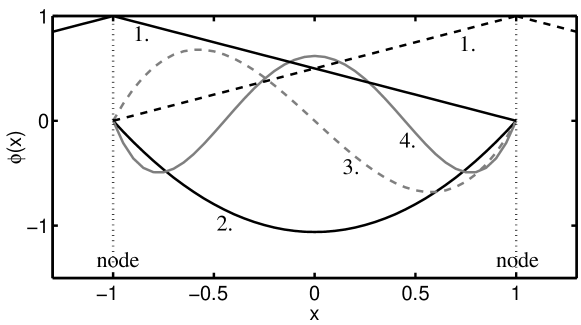
Figure 1. One-dimensional basis functions in the reference element [-1,1] up to the fourth order. Inside a element there ar two node-functions and three element-functions

The high order element includes more basis functions than the low order one. Where one tetrahedral linear element includes four linear basis functions, the fourth order one has 35. This means that the size of the elements is bigger and the overlap between basis functions is larger than in a linear mesh. Therefore when the number of the basis functions is reduced, but at the same time the filling of the coefficient matrix is increased. The filling of the matrices increases the CPU time and memory requirements when solving the equations, while the reduction of the number of basis function works in the opposite direction. However, a smooth solution converges faster for a larger filling. Therefore the critical factor for a good convergence with high-order polynomials is the smoothness of the solution. Naturally, for each problem there is an optimal polynomial order. Because the hierarchical nature of $p$-elements it is possible to change the order of the elements inside one calculation mesh. This results in the so-called $hp$ methods, where the polynomial order $p$ is variable in space as well as the size $h$ of the elements. This is useful if the nature of the solution has rapid changes in some part of the calculation area, but otherwise the solution is smooth. This is the case for example in the DFT calculations in the atomic core region.

In adaptive methods, an interesting question is how to choose whether to increase the order or decrease the element size in a given part of the mesh where resolution needs to be enhanced.

In the case of all-electron calculations, where the effective potential has a singlarity of the type $1/r$, when the same mesh is utilized for the interpolation of the effective potential and the orbitals, the standard results of approximation theory [36] suggest a refinement strategy where small elements with low order $p$ are used in the vicinity of the nuclei. In other parts of the space, the orbitals as well as the effective potential are smooth, which suggests larger and higher order elements.

Multilevel methods can be also of the “multi-$p$”-variety, where the same mesh is used at each resolution level, but the order of the elements varies.

2.4. Wavelets

The variational approximation scheme using the wavelet basis as the trial and test functions will combine the best aspects both of the FEM approach and Fourier approximation. From the FEM world we retain the locality of the approximation. For a wide class of operators their matrix representation $H$ in the wavelet basis is nearly diagonal. This fact together with the refinement equation makes it possible to carry out the matrix-vector computations in FFT speed. It can be shown that the wavelet based approximation schemes for operator equations have the optimal computational complexity in the following sense: For a given approximation tolerance $\epsilon>0$ the wavelet approximation, when computed using iterative and adaptive techniques, requires the least number of arithmetical operations and storage locations of all $N$-term approximation schemes with the same tolerance [40].

Furthermore, the wavelet transform yields powerful numerical schemes including very efficient adaptive algorithms. So the wavelet approximation is naturally adaptive. In addition to that the wavelet based approximation method combined with the multilevel techniques (i.e. the multiresolution analysis) are very good preconditioners for linear systems [41]. It can be shown for a very general class of operators that the scaled stiffness matrix has uniformly bounded condition numbers [42].

The rate of approximation depends on the smoothness of the function to be approximated and the order of the wavelets. Assuming that the solution $\psi$ of the eigenvalue problem (1) is sufficiently smooth it can be shown (see [43]) that

$$\|\psi-\psi_{h}\|_{L^{p}(\mathbb{R}^{d})}\leq c(\psi)n^{-\frac{s}{d}}.$$ (16)

Here $n$ denotes the number of basis functions on the highest resolution level of the wavelet approximation, $s$ is the approximation order of the wavelets and the constant $c(\psi)$ is independent on $n$. This approximation property is exactly the same as for the polynomial finite element spaces.

The application of wavelet analysis in $\mathbb{R}^{d}$ has been considered inpractical because the number of scaling functions increases which affects the size of the wavelet basis. This holds for the tensor product wavelets, or separable wavelets, which will be obtained from the dyadic wavelet basis in one dimensions. However, by using the non-separable wavelet basis we will retain the same situation as in one-dimensional case. We have only one scaling function. These wavelet basis will be obtained by using the isotropic scaling matrix $M$ with the determinant $\det(M)=2$, i.e. the matrix has integer coefficients. The non-separable wavelet basis have one more advantage over conventional separable wavelet functions. Because of their isotropy they are useful for rotationally invariant systems.

2.4.1. Interpolating wavelet basis set

A biorthogonal wavelet family of degree $m$ is characterized by a mother scaling function $\varphi$, a mother dual scaling function $\tilde{\varphi}$, and four finite filters $h_{j}$, $g_{j}$, $\tilde{h}_{j}$, and $\tilde{g}_{j}$. We follow the convention in [44] where the nonzero elements of the filters lie in the range $j=-m,\ldots,m$. The mother wavelet $\psi$ and the mother dual wavelet $\tilde{\psi}$ are determined by the mother scaling function, the mother dual scaling function, and the four filters.

Interpolating wavelets [45, 46, 44] are one biorthogonal wavelet family [47, 44]. Interpolating wavelets enable simple calculation of matrix elements and expansion of functions in a basis function set because of the special form of the dual scaling functions and dual wavelets. Actually the interpolating dual scaling functions and interpolating dual wavelets are not functions but distributions.

For interpolating wavelet family of degree $m$, the mother scaling function $\varphi$ is constructed by recursively applying polynomial interpolation of degree $m$ to data $s_{i}=\delta_{i,0}$ and the mother dual scaling function is

$$\tilde{\varphi}(x)=\delta(x),$$ (17)

where $\delta$ is the Dirac delta function. For interpolating wavelets the coefficients $h_{j}$ satisfy [44]

$$h_{j}=\varphi(j/2),\;\;j=-m,\ldots,m.$$ (18)

For biorthogonal wavelets the matrix elements of operators are not computed as ordinary inner products but they are computed as integrals involving the basis functions and so called dual basis functions. The matrix elements of an operator $\hat{A}$ in a basis set consisting of biorthogonal wavelets are defined by

$$A_{ij}=\int_{-\infty}^{\infty}\tilde{\zeta}_{i}(x)\;\hat{A}\;\zeta_{j}(x)dx,$$ (19)

where $\zeta_{j},\;j=1,\ldots,N$ are the basis functions, $\tilde{\zeta}_{i},\;i=1,\ldots,N$ are the dual basis functions, and $N$ is the size of the finite basis function set.

3. Linear algebra

The numerical task of solving the discretized versions of the Kohn-Sham equations, Hartree-Fock equations or equations for the Green’s functions consists of repeated solutions of linear systems of equations and/or eigenvalue problems, whereas the real-time propagation methods of TDDFT involve exponentiation of large matrices. In other words, problems of linear algebra [48]. All three discretization techniques discussed in Sec. 2 lead to sparse matrix problems. Typically these matrices are so large that it is important to store only their nonzero elements, using e.g. the CRS (Compressed Row Storage) format [49] or define the matrices only by a subroutine which operates upon a vector. Notably, in the FD-method with a uniform grid the nondiagonal elements of the discretized Laplacian are the same on each row and need not be stored.

Because of the large size of the matrices, straightforward utilization of standard linear algebra packages for dense matrices, such as Lapack [50], is not an option. Availability of a good selection of efficient tools for sparse matrix problems is thus a necessary prerequisite for large scale real-space electronic structure calculations.

It was emphasized in the notation of Eq. 4, that a part of the Hamiltonian $\hat{H}$, the effective potential $V_{\rm eff}[n]({\mathbf{r}})$, is a functional of the electron density, which on the other hand needs to be determined from the sum of the squared moduli of the occupied orbitals, which are the eigenfunctions of $\hat{H}$. We are thus presented with a nonlinear eigenvalue problem. There exists a general multigrid formulation called Full Approximation Storage (FAS) [52] which is in principle directly applicable to such nonlinear problems. Results from work on the development of nonlinear FAS eigenvalue solvers have been reported by Beck et al. [54, 55] and Costiner and Ta’asan [56]. Apart from that, one can try to minimize directly the corresponding nonquadratic total energy functional using the preconditioned steepest descent (SD) [29, 57] or conjugate-gradient (CG) [58] method, in which the electron density and hence the effective potential can be updated after each update of the approximate orbitals. However, an iterative diagonalization scheme, in which the Hamiltonian is repeatedly diagonalized for a fixed $V_{\rm eff}$, and the self-consistent $V_{\rm eff}$ is found using some “mixing scheme” in an outer loop, can be at least equally efficient [59, 60]. We have opted for the latter approach in all of our example calculations presented in Sec. 5. Some of the systems considered require special care in the choice of the mixing scheme in order to find a convergent iteration. Specifically, we want to mention here the GRPulay method [61] and the Newton-Raphson (or response function) method of Refs. [62, 63] which we have found useful in Sec. 5.5 and in Secs. 5.1 and 5.2, respectively. For more information on our recent work related to self-consistency iterations see Refs. [64, 65].

Apart from the nonlinear self-consistency problem which we solve in an outer loop, we are left with only standard problems of linear algebra. The problems relevant for our work can be divided in three classes: systems of linear equations (Sec. 3.1), eigenvalue problems (Sec. 3.2) and matrix exponentiation, which is needed in time propagation schemes [66], as briefly discussed in Sec. 6.1.

3.1. Systems of linear equations

Large linear systems of equations occur in real-space electronic structure calculations in many contexts. In the example calculations of Sec. 5 the discretized Poisson equation, the inversion step in the shift and invert mode of the Lanczos method (Sec. 3.2.1), the equations of full-response (Eq. 30) and collective approximation ([63]) formulations of the response function method, and the matrix inversion for obtaining the Green’s function from Eq. 36 (after discretization with the finite-element method) occur. Usually it is most convenient to solve such systems with iterative methods [67]. However, for matrix inversion, where the same equation has to be solved many times with different right-hand sides, direct methods are more efficient.

3.1.1. Iterative solvers

For symmetric positive definite matrices, the conjugate gradient (CG) method is often the standard choice. For the dense “matrix-free” problems occuring in the application of the response function method to two-dimensional quantum dot problems (Sec. 5.1) the CG method was found efficient even in the absence of any preconditioner.

Often, however, it is important to accelerate the convergence of the CG method through preconditioning. Preconditioning the equation $Ax=b$ corresponds to multiplying the equation by an approximate inverse $B\approx A^{-1}$, resulting in $x\approx BAx=Bb$. In our applications of the finite-element method to all-electron calculations of molecules (Sec. 5.4) the CG method with preconditioners based on incomplete LU factorization (ILU) [68] and the multigrid method [69, 70, 71] was applied to the linear system of equations occuring in the inversion step of the shift and invert mode of the Lanczos method for the eigenvalue problem (see Sec. 3.2.1).

A multigrid method where the Gauss-Seidel method is used as a smoother, is used as a solver for the linear system of equations that results from the FD-discretization of the Poisson equation within the MIKA-package [64, 65].

In the axial symmetry, the matrix for the Laplacian within the FD-method is not symmetric. However, we have found that our MG-method with the Gauss-Seidel method as a smoother converges. On the other hand, the CG-method for the full-response equation 30 is not applicable. The best method we could find for this problem was the GMRES method with no preconditioning [67]. For the corresponding equation of the collective approximation [63] we found no useful iterative scheme. This problem obviously calls for further work. A good starting point is probably to take a look at the algorithms available in the Sparskit package [51].

3.1.2. Direct solvers

When solving for the inverse of a matrix as is the case in the calculations employing the Green’s function (see Sec. 5.5) it is not usually feasible to use iterative methods since the iteration must usually be performed separately for each column of the inverse. Instead, direct methods for sparse matrices provide an attractive alternative since part of the computational work needs to performed only once per inverse. Modern direct methods for sparse matrices are based on the frontal factorisation algorithm of the sparse matrix [72, 73]. The algorithm starts with symbolic factorisation of the matrix, i.e. heuristically finding a permutation that is intended to minimise the fill-in in the numerical factors. Next, a sparse Cholesky or LU-factorisation is computed using block operations with dense BLAS kernels. Finally the problem is solved with backward and forward substitutions. If the entire inverse is desired only the final substitution steps must be performed for each column of the inverse whereas the matrix factors remain unaltered. Several implementations of the frontal method are available as software libraries, e.g. [74, 75, 76].

3.2. Eigenproblem solvers

Mostly these eigenproblems are Hermitian, so that Lanczos based iterations are the starting point, if one looks at the problem from the point of view of a numerical analyst [77]. For physicists the starting point is often the preconditioned conjugate gradient method (PCG) [58]. Also nonhermitian eigenvalue problems sometimes occur. This happens e.g. when generalized finite-difference discretizations are used (e.g. the Mehrstellen discretization of Ref. [29, 57]), if the method of adaptive coordinates is applied without extra care to guarantee symmetric matrices [79, 5], and also when the FD-method is applied in axial symmetry [80].

In this section we describe those eigenproblem solvers that are used in the example calculations of Sec. 5, as well as the residual minimization method (Sec. 3.2.3), which is at the core of the GridPaw-code (Sec. 4.3), on which the main line of development within the MIKA-project is currently based on.

This is not an exhaustive list of eigenproblem solvers. In finite-difference based electronic structure calculations also the method of steepest descent with multigrid preconditioning on global grids [29, 57] as well as in an almost linear scaling implementation based on localized orbitals (support functions presented on a grid) [13] is used. The highly efficient method utilized in Parsec is based on a taylor-made parallel generalized Davidson method [81]. Recently, a new preconditioned, Krylov-space technique has been introduced in the mathematical litterature by A. Knyazev [82, 83] – this method is claimed to be more efficient than its precursors, and certainly deserves to be properly tested in challenging applications. Relatively large and dense eigenvalue problems of a different structure occur when computing excitation energies and oscillator strengths from TDDFT from the Casida equation [84, 85]. Here, the Davidson method [86, 87] is often used [88, 89] for finding a few of the lowest excitation energies. According to Ref. [90], however, it is also feasible to utilize the Lapack [50] or ScaLapack [91] routines for all eigenvalues of dense matrices in this case.

3.2.1. Lanczos and Arnoldi methods

The Arnoldi Package Arpack [92] contains an implementation of the Lanczos method as well as its generalization to nonsymmetric problems, the Arnoldi method. It is used through a reverse communication user interface, i.e. the user has to provide his or her own subroutines for matrix-vector products and solvers for linear systems of equations, and Arpack calls these user defined subroutines when needed. Thus the efficiency of Arpack actually depends heavily on the efficiency of these user defined subroutines.

We have used Arpack in the so-called shift and invert mode in the finite-element example calculations presented in Sec. 5.4. The computationally expensive step in these calculations was the solution of a linear system of equations, for which the CG-method was applied as discussed above in Sec. 3.1.1.

3.2.2. Rayleigh-quotient multigrid

The Rayleigh-quotient multigrid (RQMG) method [93] is originally developed for the generalized eigenproblem

$$H{\bf u}=\epsilon B{\bf u}$$ (20)

that arises from a FD-discretization of an equation of the form of Eq. 1. Unless generalized finite-difference methods (such as those of Refs. [29, 30, 31]) are used, $B=I$ and $H$ is Hermitian (in fact real and symmetric). In the general case, it is assumed that $B^{-1}H$ is Hermitian, thus the eigenvectors are orthonormal in $\mathbb{R}^{N}$: ${\bf u}_{i}^{H}{\bf u}_{j}=\delta_{ij}$. Given the eigenvectors $\{{\bf u}_{i};1\leq i\leq k\}$, ${\bf u}_{k+1}$ is obtained by finding the minimum of the functional

$$F[{\bf u}_{k+1}]=\frac{{\bf u}_{k+1}^{H}H{\bf u}_{k+1}}{{\bf u}_{k+1}^{H}B{\bf u}_{k+1}}+\sum_{i=1}^{k}q_{i}\frac{\left|{\bf u}_{i}^{H}{\bf u}_{k+1}\right|^{2}}{{\bf u}_{i}^{H}{\bf u}_{i}{{\bf u}_{k+1}^{H}{\bf u}_{k+1}}}.$$ (21)

In the minimization process, a hierarchy of grids is utilized, and on each grid, one degree of freedom is varied at a time and the minimum of the functional is found along the corresponding line in the space of u’s. Varying one degree of freedom on a coarse grid corresponds to varying the u values at multiple grid points on the fine grid at the same time. More details on the RQMG method can be found from Refs. [93, 94, 80, 64, 65]. Our implementation of the RQMG method was motivated by the method due to Mandel and McCormick [95], which was designed for the solution of the eigenvector with lowest eigenvalue from a generalized eigenproblem derived from a finite-element discretization.

3.2.3. Residual minimization method

Variants of the residual minimization method of Wood and Zunger [96] are used as eigensolvers in the plane-wave code VASP [59, 60] as well as in the FD-PAW package GridPaw [97]. The basic idea is to update the orbitals at each iteration by taking a step along the preconditioned residual $P{\bf R}_{n}$:

$${\bf u}^{\prime}_{n}={\bf u}_{n}+\lambda P{\bf R}_{n}.$$ (22)

The residual is defined as

$${\bf R}_{n}=(H-\varepsilon_{n}S){\bf u}_{n},$$ (23)

where $\varepsilon_{n}$ is the present estimate of the eigenvalue computed as the Rayleigh quotient, and the preconditioner $P$ is discussed below. $\lambda$ is chosen such that the residual ${\bf R}^{\prime}_{n}$ at the new guess ${\bf u}^{\prime}_{n}$

$${\bf R}^{\prime}_{n}=(H-\varepsilon_{n}S){\bf u}^{\prime}_{n}={\bf R}_{n}+\lambda(H-\varepsilon_{n}S)P{\bf R}_{n}$$ (24)

is minimized. This amounts to finding the minimum of a second order polynomial in $\lambda$. In the implementation of Ref. [97], an additional step is then performed by taking also a step of length $\lambda$ in the direction of $P{\bf R}^{\prime}_{n}$

$${\bf u}_{n}\leftarrow{\bf u}_{n}+\lambda P{\bf R}_{n}+\lambda P{\bf R}^{\prime}_{n}.$$ (25)

In the implementation of Refs. [59, 60] the residual is minimized in a multidimensional space spanned by the present guess ${\bf u}_{n}$ and several preconditioned residuals from previous iterations - thus the name RMM-DIIS (Residual metric minimization with direct inversion in the iterative subspace). The general idea of minimizing a (preconditioned) residual in a multidimensional space spanned by previous residuals is the same as in the well-known Pulay (DIIS) mixing schemes [98, 99, 59, 60, 61].

The optimal preconditioned residual would be obtained by solving $\tilde{\bf R}_{n}=P{\bf R}_{n}$ from $(H-\varepsilon S)\tilde{\bf R}_{n}={\bf R}_{n}$. In Ref. [97] one solves instead approximately the simpler equation $-\frac{1}{2}\nabla^{2}\tilde{\bf R}_{n}={\bf R}_{n}$ with the aid of a single multigrid V-cycle.

3.2.4. Diffusion algorithm

In connection with the program package developed in the group of Prof. Eckhard Krotscheck (see Sec. 4.2) the lowest $n$ solutions of the single-electron Schrödinger equation are solved by applying the evolution operator, $\mathcal{T}(\epsilon)\equiv\text{e}^{-\epsilon H}$, repeatedly to a set of states $\{\psi_{j},\,1\leq j\leq n\}$, and orthogonalizing the states after every step. Instead of the commonly used second-order factorization in combination with the Gram-Schmidt orthogonalization, the fourth-order factorization for the evolution operator [100] is used. It is given by

$$\mathcal{T}^{(4)}\equiv\text{e}^{-\frac{1}{6}\epsilon V}\text{e}^{-\frac{1}{2}\epsilon T}\text{e}^{-\frac{2}{3}\epsilon\tilde{V}}\text{e}^{-\frac{1}{2}\epsilon T}\text{e}^{-\frac{1}{6}\epsilon V}=\text{e}^{-\epsilon[H+\mathcal{O}(\epsilon^{4})]};\qquad\tilde{V}=V+\frac{1}{48}\epsilon^{2}[V,[T,V]],$$ (26)

where one operates with the potential energy operators $V,\tilde{V}$ in real-space, and with the kinetic energy operator $T$ in the $k$ space. Switching between spaces is expedited via fast fourier transforms (FFT). Instead of Gramm-Schmidt orthogonalization, the Hamiltonian is diagonalized in the subspace of present approximate solutions and a new set of orthonormal states is thereby obtained. This step, often referred to as a subspace rotation, is in fact an application of the Petrov-Galerkin method of Sec 2.2 with the present approximate solutions as basis functions.

Depending on the physical system this method can be faster by up to a factor of 100 in comparison to the second-order factorization.

4. Six projects

This paper collects together material from essentially three separate lines of work. One of them is the MIKA project (see Sec. 4.1), which is in fact an umbrella for a number of activities related to real-space methods. The first priority in the MIKA-project is on the expansion of these activities to include also time-dependent problems. The MIKA-project has already spawned important international collaborations with two other projects (see Secs. 4.2 and 4.3). Another line of work is defined by its aim to promote the applications of the finite-element methods in electronic structure calculations. Actual work related to the finite-element approach has been performed with two codes - one of them is the well established general purpose Elmer package (see Sec. 4.4) developed at CSC, and the other one has been recently developed for transport calculations (see Sec. 4.5). The third and thus far entirely independent line is centered around the wavelet approach (see Sec. 4.6).

4.1. MIKA - a project and a program package

The finite-difference program package MIKA has been described in Refs. [94, 64, 65]. Example calculations using its components are described in those references as well as in Secs. 5.1, 5.2 and 5.3 of this article. The common denominator of these programs is the utilization of the RQMG-method (Sec. 3.2.2, Ref. [93]) as an eigensolver. The MIKA-package can be downloaded freely from the internet at http://www.csc.fi/physics/mika/.

The MIKA-project, on the other hand should not be understood as too tightly bound to the MIKA-package. Instead, it is a project for the development of real-space methods in general, and currently the main emphasis is on the expansion of the activities to dynamic phenomena described by the time-dependent density-functional theory (TDDFT) [3]. We have chosen the GridPaw-code (Sec. 4.3) as the basis for this development, although we, at the same time, monitor the development of the alternative FE-approach based on the Elmer-package (Sec. 4.4).

4.2. Diffusion-algorithm and response-function package

The real-space program package developed at the University of Linz [62, 100, 63, 101, 102] for solving the KS equations can be thought as an alternative to the approach used in MIKA. Instead of using multigrid methods, the eigenvalue problem is solved in this program by using a diffusion algorithm, namely a highly efficient fourth-order factorization of the evolution operator (see Sec. 3.2.4). Secondly, the number of self-consistent iterations is significally reduced by applying a response-function method. Within the MIKA package, the response-function algorithm has been implemented into MIKA/cyl2 (see Sec. 5.2). The research applications of the two programs to quantum dot studies have been rather similar, and the latest research results summarized in Sec. 5.1 have largely originated from collaborations between the two projects.

4.3. GridPaw

Also the GridPaw code developed in the Center for Atomic-scale Materials Physics (CAMP) of the Technical University of Denmark is a finite-difference program package for the Kohn-Sham equations, in which strategies different from those in the MIKA -package have been chosen [97]. Instead of norm-conserving pseudopotentials, the Projector Augmented Wave (PAW) approach [9, 10] is implemented. A very important technical detail in this implementation is the utilization of the double-grid method [16], discussed in Sec. 2.1. Instead of the RQMG method, the residual minimization method with multigrid preconditioning is applied to solve the eigenvalue problem as described in Sec. 3.2.3. Within the second phase of the MIKA-project, a close collaboration with the GridPaw project is essential, as described in Sec. 6.1.

4.4. Elmer

Elmer is a general purpose finite element solver and collection of library subroutines for solving systems of partial differential equations by the finite element method.

Given a finite element partition of an $n$-dimensional computational domain, the program automatically constructs graphs for system matrices in the compressed row storage format, optimizes bandwidth, builds up the quadtree search structures and, if required, the restriction and extension operators for projecting functions between different levels of finite element spaces in multigrid analysis.

The program provides interpolation basis functions and their gradients for simplices and $n$-cubes for any given polynomial degree up to ten, and automatically determines the optimal quadrature for numerically evaluating their inner products. The local element matrices representing the disretized differential operators are finally assembled in global structures using the predetermined graphs. The global system is solved either with standard multifrontal decomposition methods or Krylov-type iteration schemes. The iterative solvers may be preconditioned by standard incomplete decompositions, or multigrid methods. For eigenvalue problems the program utilizes the Arnoldi-method as implemented in the Arpack -package [92] in the shift-and-invert mode, with its own linear system solvers applied to the computationally expensive invertion-step of the algorithm.

Basically, the program is well suited for solving problems that can be posed in variational form. The classical Kohn-Sham scheme of DFT, for example, fits into this framework extremely well. So far, we have performed some preliminary tests for computing the electronic charge density for simple molecules like CO and C₆₀ (see Sec. 5.4). The results of these all-electron calculations are promising, but there is some work that could be done to enhance the overall performance of the code. The major problems are not in the finite element discretization itself, but in the performance of the eigenvalue solver, and the relaxation techniques needed to avoid the charge sloshing phenomenon of the Kohn-Sham scheme. Here one can directly utilize experience gathered using more traditional discretization schemes (see Sec. 3).

For more information, see http://www.csc.fi/elmer/.

4.5. Finite-element method for electron transport

The program for modeling transport properties of the nanostructures is written in the Laboratory of Physics within a co-operation with the Institute of Mathematics both in the Helsinki University of Technology. The project is in detail presented in the thesis [103].

A nanostructure between leads is a typical electron transport problem. This kind of systems are problematic to the DFT with eigenfunction methods, because the system is of infinite size without periodicity. We have solved this problem using the Green’s function methods with the open boundary conditions. The code has three versions: one-, two-, and three-dimensional, so that different types of nanostructures can be modeled. The numerical implementation is done using the finite-element method with $p$-elements up to the fourth order. We use mesh generator Easymesh [38] in the two-dimensional calculations, and Netgen [14] in the three-dimensional ones.

4.6. Wavelet package

The interpolating wavelet package for the computation of the atomic orbitals has been written in the Institute of Physics in the Tampere University of Technology in co-operation with the Mathematics Division of the Faculty of Technology from the University of Oulu. The aim of the effort is to develop the wavelet method for the quantum mechanical applications. Instead of using the orthogonal Daubechies wavelets the biorthogonal interpolating wavelets have been utilized in the implementation of the code. Up to now the atomic orbitals have been computed for some light many-electron atoms (ions). In the implementation we have used the nonstandard operator form, since it provides an efficient method to carry out the multi-resolution analysis in the electronic structure calculations.

5. Calculation examples

In this section we present example calculations from each of the three lines of work. The MIKA-project emphasizes the finite-difference method, and thus far has also been centered on the MIKA-package [64, 65]. Applications of this package to quantum dots, surface nanostructures and positron calculations are presented in Sections 5.1, 5.2 and 5.3, respectively. Note, however, that many of the results reported in Sec. 5.1 have been calculated with the response function package described in Sec. 4.2. The introduction of the finite-element method to electronic structure problems materializes in Sec. 5.4, where all-electron calculations for CO and C₆₀ are presented, and in Sec 5.5, where transport calculations based on the nonequilibrium Green’s functions with norm-conserving pseudopotentials are presented. Preliminary results of our implementation of the wavelet approach to electronic structure calculations are presented in Sec. 5.6.

5.1. Recent real-space calculations on two-dimensional quantum dots

In this Section we present a brief review on our recent computational results for two-dimensional quantum dots (QD’s) [104]. We consider QD’s fabricated at the interfaces of semiconductor heterostructures (e.g. GaAs/AlGaAs), where the two-dimensional electron gas (2DEG) is restricted. The many-electron Hamiltonian for a QD in the presence of a magnetic field is written in SI units as

$$H=\frac{1}{2m^{*}}\sum^{N}_{i=1}\left[-i\hbar\nabla_{i}+e\mathbf{A}({\mathbf{r}}_{i})\right]^{2}+\sum^{N}_{i<j}\frac{e^{2}}{4\pi\epsilon_{0}\epsilon|{\mathbf{r}}_{i}-{\mathbf{r}}_{j}|}+\sum^{N}_{i=1}\left[V_{\rm ext}({\mathbf{r}}_{i})+g^{*}\mu_{B}Bs_{z,i}\right],$$ (27)

where the vector potential is chosen in the symmetric gauge to define the magnetic field perpendicular to the dot plane. We use the effective-mass approximation with the material parameters for GaAs, i.e., the effective mass $m^{*}$=0.067 $m_{e}$ and the dielectric constant $\epsilon=12.4-13$. The external confining potential is determined by $V_{\rm ext}({\mathbf{r}})$ and the last term is the Zeeman energy.

In the calculations we apply the SDFT in the self-consistent KS formulation. In high magnetic fields we have also employed the computationally more demanding current-spin-density-functional theory (CSDFT), which does not, however, represent a considerable qualitative improvement over the SDFT. A detailed comparison between these two methods for a six-electron quantum dot can be found in Ref. [105].

In the numerical process of solving the KS equations we have used both the response-function package (see Sec. 4.2) as well as the 2D version of the MIKA package (MIKA/RS2dot). Recent QD applications studied using these methods can be found in Secs. 5.1.1 and  5.1.2, respectively. Within the both methods, the effective single-electron Schrödinger equation is solved on a two-dimensional point grid. In practical calculations, the number of grid points is set between 128 and 196 in one direction. This gives less than $\sim 1$ nm for a typical grid spacing, which is sufficient for describing electrons in GaAs. Within MIKA/RS2dot, obtaining full convergence typically takes $100\dots 500$ self-consistency iterations. By using the response-function methods this number can be typically reduced by a factor of ten.

5.1.1. Statistics of quantum-dot ensembles

We have applied the response-function algorithm presented in the previous section to study the statistical properties of quantum dots (in zero magnetic fields) affected by external impurities [106, 107]. In the Hamiltonian given in Eq. 27 the external potential $V_{\rm ext}({\mathbf{r}})$ consists of a parabolic confinement $V_{\rm c}(r)=m^{*}\omega_{0}^{2}r^{2}/2$ with and the impurity potential

$$V_{\rm imp}({\mathbf{r}})=\sum^{N_{\rm imp}}_{k=1}\frac{-e}{4\pi\epsilon\epsilon_{0}\sqrt{({\mathbf{r}}-{\mathbf{R}}_{k})^{2}+d^{2}_{k}}},$$ (28)

where $N_{\rm imp}$ is the number of impurities and ${\mathbf{R}}_{k}$ and $d_{k}$ are their (random) lateral and vertical positions in the ranges of $0\leq R_{k}\leq 100\,{\rm nm}$ and $0\leq d_{k}\leq 10\,{\rm nm}$, respectively. For each fixed $N_{\rm imp}=5\ldots 50$ we apply 1000 random impurity configurations.

In a noninteracting system the addition energy for a certain electron number $N$ is equal to the eigenlevel spacing, i.e., $\Delta_{0}(N)=\epsilon_{N/2+1}-\epsilon_{N/2}$, where the divisor of two follows from the spin degeneracy. We have shown that in this case the resulting addition-energy distribution is a combination of Poisson and Wigner-Dyson distributions, corresponding to regular and chaotic systems, respectively [106].

In the interacting many-electron system the addition energy is given as the second energy difference, $\Delta(N)=E(N-1)-2E(N)+E(N+1)$. The ground-state energies are chosen from the spin states with lowest energies. We calculated all the relevant spin configurations for different electron numbers $N$, so that taking the impurity configurations into account, a total number of $\sim 10^{5}$ self-consistent SDFT calculations were performed. We note that this would not have been manageable (in a reasonable time) using conventional mixing schemes in solving the KS equations.

There is an essential difference in the addition-energy behavior of noninteracting and interacting systems as a function of $N_{\rm imp}$. Namely, when the impurity number is increased the distribution of the interacting system becomes symmetrical with Gaussian tails. This result is qualitatively similar to what has been found in experiments for large QD’s [108, 109], as well as with previous DFT calculations for disordered QD’s [110, 111]. The result demonstrates the necessity for comprehensive treatment of the e-e interactions beyond the random matrix theory combined with the constant-interaction model. In our system, the approximate impurity density required for the symmetrization of the addition-energy distribution is $\sim 10^{-3}\,{\rm nm}^{-2}$, which is of the same order of magnitude as the one used by Hirose et al. [110] in their calculations of disordered QD’s.

We have also analyzed the dependence of the spin states on the impurity density and on the corresponding noninteracting level statistics [107]. Figure 2

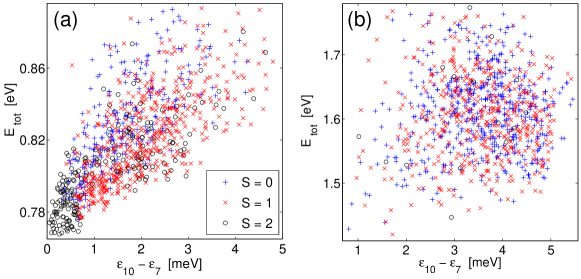
Figure 2. (Color online) Total energy for different spin states in a 16-electron quantum dot vs. the sum of the noninteracting level splittings on the fourth energy shell. The number of impurities are $N_{\rm imp}=5$ (a) and $N_{\rm imp}=20$ (b). Reprinted with permission from E. Räsänen and M. Aichinger, Phys. Rev. B 72, 045352 (2005). Copyright (2005) by the American Physical Society.

shows the ground-state spins ($S=0,1,2$) for a 16-electron QD with four impurity numbers $N_{\rm imp}=5$ (a) and $20$ (b). The results are shown in a plane spanned by the sum of the level splittings on the fourth shell, $\epsilon_{10}-\epsilon_{7}$, and the total energy $E_{\rm tot}$. The fraction of the $S=2$ states strongly decreases as $N_{\rm imp}$ is increased. However, the relation of the $S=0$ and $S=1$ states gradually saturates toward one. The saturation effect is analyzed in Ref. [107] in detail. In the case of a small impurity density, the resulting spin states show strong statistical dependence on the level splittings: when the level spacing is small, partial spin polarization is probable due to Hund’s rule. This applies especially for $S=2$ states which are clustered in Fig. 2(a). However, when the impurity density is increased the spin-state correlation totally disappears. This indicates that in strongly distorted systems the spin of the many-electron ground state can not be predicted from the single-electron spectrum due to the complicity of the e-e interactions.

5.1.2. Quantum Hall regime

The real-space method based on MIKA/RS2dothas proven to be a reliable and efficient density-functional approach to study finite 2D electron systems in magnetic fields [112, 113, 114, 115, 116]. The original inspiration for our work is related with the well-known quantum Hall effect in 2DEG [117], as well as in the electron transport [118] and magnetization [119] measurements, which both have revealed a rich variety of transitions in the energetics of finite electron systems as a function of the magnetic field.

We have recently shown using both the SDFT and the exact diagonalization (ED), that in QD’s representing finite-size quantum Hall droplets at strong magnetic fields the off-electron zeros may localize [112]. In a parabolic confinement, vortices form stable, clustered configurations with successive transitions between them, as the magnetic field (and thus angular momentum) is increased [112, 120]. The mean-field SDFT densities and the conditional wave functions of the ED results shows similar vortex structures. Furthermore, QD’s defined by a non-circular, e.g., elliptic or rectangular confining potential, exhibit a good agreement between the total densities obtained with SDFT and ED calculations, respectively [113]. Figure 3

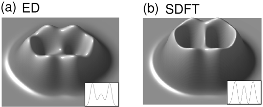
Figure 3. Electron densities (gray scale) for two-vortex solutions in elliptical quantum dots (${\rm eccentricity}=1.2$) calculated using the ED (a) and SDFT within MIKA/RS2dot(b). Reprinted with permission from H. Saarikoski et al., Phys. Rev. B 71, 035421 (2005). Copyright (2005) by the American Physical Society.

shows the electron density obtained using the ED (a) and SDFT (b) for two-vortex solutions in elliptical QD’s. In the SDFT results the vortices are strongly localized with the electron density close to zero in the core, which reflects the fact that the mean-field method is not able to include all the correlations of the exact many-body state. We have found similar differences between the ED and SDFT for the so-called giant-vortex states, which are formed if a quartic term (flatness) is included to the otherwise parabolic potential [115].

The state transitions in the quantum Hall regime are also visible as oscillations in the QD energetics, e.g., in the chemical potentials $\mu(N)=E(N)-E(N-1)$ (Ref. [114]). At magnetic fields below the total spin polarization we have found finite-size counterparts of the integer and half-integer quantum Hall states, as well as a developing pattern of de Haas–van Alphen oscillations in the magnetization $M(N)=-\partial E(N)/\partial B$ (Ref. [116]). These results are qualitatively consistent with the experimental magnetization data of large dot arrays [119]. At higher magnetic fields the signatures of above discussed vortex formation inside the QD are clearly visible in the magnetization oscillations, and the agreement between the SDFT and QMC results is good. These oscillations should be observable in accurate magnetization measurements of QD devices.

5.2. Surface nanostructures studied with MIKA/cyl2

5.2.1. Calculations in axial symmetry

Many interesting nanostructures, such as adatoms on the surfaces, circular quantum dots and quantum corrals can be modelled in axial symmetry. Numerically the problem is reduced from 3D to 2D which makes the calculations drastically easier, and allows modelling of much larger systems.

In an axially symmetric potential the Schrödinger equation written in the cylindrical coordinates is separable. The Kohn-Sham orbitals are given as a product of the angular and (r,z) -dependent parts, i.e.,

$$\psi_{mkn}(\mathbf{r})=e^{im\phi}U_{mkn}(r,z).$$ (29)

The formalism is nice from the computational point of view as the eigenstates with different $m$ and $\mathbf{k}$ are automatically orthogonal. This allows the problem to be splitted into various subproblems and we can take the full advantage of massively parallel computing environment.

It is noteworthy that we can make use of this special form of wave functions also in the response-function scheme. The density correction is determined from Eq. (2.5) of Ref. [62], which reads after writing out the dielectric function,

$$\Delta\rho^{\left(k\right)}(\mathbf{r})-\delta\rho^{(k)}(\mathbf{r})=2\sum_{p,h}\frac{\psi_{p}(\mathbf{r})\psi_{h}(\mathbf{r})}{\epsilon_{p}-\epsilon_{h}}\int d^{3}r^{\prime}d^{3}r^{\prime\prime}\psi_{p}(\mathbf{r}^{\prime})\psi_{h}(\mathbf{r}^{\prime})V_{p-h}(\mathbf{r}^{\prime},\mathbf{r}^{\prime\prime})\delta\rho^{(k)}(\mathbf{r}^{\prime\prime}).$$ (30)

Inserting (29) and rewriting the integrals in the cylindrical coordinates we see that the integral over $r^{\prime}$ happily vanishes unless the wave functions share the same angular momentum quantum number. This drastically reduces the number of terms in the above summation which is welcome when one tries to solve the linear equation using an iterative method such as conjugate gradient or GMRES where efficient calculation of the matrix operator is essential. Furthermore, “particle-hole interaction” $V_{p-h}$ can also be crudely approximated by the Coulomb part of the effective potential (remember that it does not affect the final result, only the speed of the iteration process), i.e., $V_{p-h}(\mathbf{r},\mathbf{r}^{\prime})\approx\frac{\delta V_{c}(\mathbf{r})}{\delta\rho(\mathbf{r}^{\prime})}$. Thus the integration over double primed coordinate gives just the electrostatic potential “caused” by the charge distribution $\delta\rho^{(k)}(\mathbf{r}^{\prime})$,

$$\int dr^{\prime}\frac{\delta V_{c}(\mathbf{r})}{\delta\rho(\mathbf{r}^{\prime})}\delta\rho^{(k)}(\mathbf{r}^{\prime})=\int dr^{\prime}\frac{\delta\rho^{(k)}(\mathbf{r}^{\prime})}{\left|\mathbf{r}-\mathbf{r}^{\prime}\right|}=V(\mathbf{r}),$$ (31)

so that the time consuming second integration can be circumvented by simply solving the corresponding Poisson equation, $\nabla^{2}V(\mathbf{r})=-4\pi\delta\rho(\mathbf{r}),$ that can be done efficiently in the axial symmetry. With the response-function scheme we have been able to solve self-consistently electron systems consisting of over 10000 Kohn-Sham orbitals in approximately 100 cpu hours with IBMpower4 processors.

5.2.2. Cu(111) surface and structures

The Cu(111) surface is an example of a crystallographic cut of the material that places the Fermi energy of electrons propagating normal to the surface inside the bulk bandgap. Conduction electrons on the surface have energy close to the Fermi energy and are sandwiched on the surface, unable to escape into the vacuum because of the potential barrier, and forbidden to enter the bulk because of the band gap. They can however move parallel to the surface and thereby form a kind of two-dimensional electron gas. Adatoms deposited on the surface can affect the surface electron distribution, which offers interesting possibilities to study the properties of confined electrons, their interaction with adsorbates and many-body physics in general.

We have used the MIKA/cyl2  software to study axial symmetric surface structures such as single adatoms and circular quantum corrals. The Cu substrate in our calculations is described by a 1D model potential; the Cu(111) planes, perpendicular to our symmetry axis (z), are considered to have uniform density, while in the z-direction we have an oscillating periodic potential that mimics the periodic structure. This particular model was proposed by Chulkov et al. [121]. In addition to the work function and the bandgap, the model potential produces correctly the Shockley surface states and the image-potential states. Previously, this model has been successfully used e.g. in studies of dielectric response-functions and lifetimes of excited states [122], and electron confinement in a metallic slab on solid surfaces within 1D self-consistent DFT calculations [123]. Once the surface is constructed, suitable pieces of jellium can be added to mimic various kinds of adsorbates.

So far we have studied e.g. the behaviour of surface state wave functions when a single Pb-adatom is deposited on the surface. On the plain surface the state is delocalized and has a constant amplitude along the surface, where as with Pb-adatom, it is localised in the Pb adsorbate (Fig.4). In a more complex case we have examined surface state electrons inside a circular ring of adatoms deposited on the surface. These kind of quantum corrals have been extensively studied experimentally and theoretically within the scattering theory, where oscillations on the surface LDOS have been observed [124]. Our calculations represent a somewhat different viewpoint as the LDOS is calculated starting from the Kohn-Sham orbitals instead of the scattering Green function.

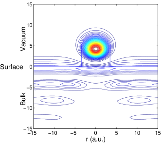
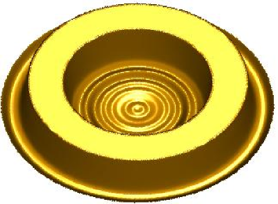
Figure 4. Two example calculations with MIKA/cyl2. Left: modulus of the first surface state wave function localized at the single Pb adatom deposited on the Cu(111) surface. Jellium profile of the adsorbate is pictured with the rectangular box. Right: 3D picture of the oscillations of the surface electron density inside a small, circular quantum corral.

5.3. Positron calculations with MIKA/doppler

The use of positron annihilation in defect studies is based on the trapping of positrons from a delocalized bulk state to a localized state at the defect (see Fig. 5a). The trapping is due to the reduced nuclear repulsion at the open-volume defects. Because the electronic structure seen by the positron at the defect differs from that in the perfect bulk crystal the annihilation characteristics change. The positron lifetime increases because the average electron density decreases. For the same reason the momentum distribution of annihilating electron-positron pairs becomes more peaked at low momenta. However, the positron density may sample the different atomic species of a compound material with different relative probabilities in the bulk and at a defect. The defect may be surrounded by impurity atoms. In these cases the high-momentum region of the distribution, which is mainly due to annihilation with core electrons, reflects the chemical structure of the defect. The changes in the bond structure between the atoms neighboring the defect may also affect the low-momentum part of the distribution. In order to understand these changes and fully benefit from them in defect identification, theoretical calculations with high predictive power are indispensable.

The description of the electron-positron system can be formulated as a two-component density-functional theory [125]. In the measurements there is only one positron in the solid sample at a time. Therefore, the density-functional scheme has to be properly purified from positron self-interaction effects. Comparisons between theoretical two-component DFT results and experimental results have shown that the following scheme is adequate. First, the electron density $n(\mathbf{r})$ of the system is solved without the effect of the positron. This can be done using different (all-electron) electronic structure calculation methods. A surprisingly good approximation for the positron lifetime and core-electron momentum calculations is to simply superimpose free atom charges. Then the potential $V_{+}(\mathbf{r})$ felt by positron is constructed as a sum of the Coulomb potential $\phi(\mathbf{r})$ due to electrons and ions and the so-called (electron-positron) correlation potential $V_{\mathrm{corr}}(\mathbf{r})$ which is treated in a local density approximation (LDA). In the zero-positron-density limit it is a function of the electron density $n_{-}(\mathbf{r})$ only, i.e.

$$V_{+}({\bf r})=\phi({\bf r})+V_{\mathrm{corr}}(n_{-}({\bf r})),$$ (32)

The ensuing single-particle Schrödinger equation can be solved using similar techniques as used for the electron states. For example, we use the three-dimensional real-space Schrödinger equation solver of the MIKA package. When using self-consistent electronic charge density we use also the Poisson equation solver of the MIKA package to calculate in Eq. (32) the Coulomb potential due to valence electrons.

The scheme described above is for a delocalized positron the exact zero-positron-density limit of the two-component DFT. However, the approximation made in the case of a localized positron can be justified by considering the positron and its screening cloud as a neutral quasiparticle which does not affect the average electron density.

When the electron density $n(\mathbf{r})$ and the positron density $n_{+}(\mathbf{r})=|\psi^{+}(\mathbf{r})|^{2}$ are known the positron annihilation rate is calculated within the LDA (in the zero-positron-density limit) as an overlap integral

$$\lambda=\frac{1}{\tau}=\pi r_{e}^{2}c\int\mathrm{d}{\bf r}\,n_{+}({\bf r})n_{-}({\bf r})\gamma(n_{-}({\bf r})),$$ (33)

where $r_{e}$ is the classical electron radius, $c$ the speed of light, and $\gamma$ the enhancement factor taking into account the pile-up of electron density at the positron (a correlation effect). The inverse of the annihilation rate is the positron lifetime $\tau$.

We calculate the momentum distribution of the annihilating electron-positron pairs using the so-called state-dependent enhancement scheme [126] as

$$\rho({\bf p})=\pi r_{e}^{2}c\sum_{j}\gamma_{j}\bigg{|}\int\mathrm{d}{\bf r}\,e^{-{\rm i}{\bf p}\cdot{\bf r}}\psi^{+}(\mathbf{r})\psi_{j}(\mathbf{r})\bigg{|}^{2},$$ (34)

where the state-dependent enhancement factor is written as $\gamma_{j}=\lambda_{j}/\lambda_{j}^{\mathrm{IPM}}$. $\lambda_{j}$ is the annihilation rate of the state $j$ within the LDA,

$$\lambda_{j}=\pi r_{e}^{2}c\int\mathrm{d}\mathbf{r}\,n_{+}(\mathbf{r})n_{j}(\mathbf{r})\gamma(n_{-}(\mathbf{r})),$$ (35)

and $\lambda_{j}^{\mathrm{IPM}}$ is the annihilation rate of the state $j$ within the independent-particle model (IPM, $\gamma\equiv 1$). Above, $n_{j}(\mathbf{r})=|\psi_{j}(\mathbf{r})|^{2}$ is the electron density of the state $j$. One can directly compare computational results with experimentally measured Doppler broadening of the 511 keV annihilation line or with experimentally measured angular correlation of the annihilation gammas. We have found that the use of the commonly employed position-dependent enhancement factor [enhancement taken into account with the factor $\sqrt{\gamma(n_{-}(\mathbf{r}))}$ inside the Fourier transform in Eq. (34)] leads to unphysical results when one compares the ratio of two Doppler spectra with the experiment [127].

a)

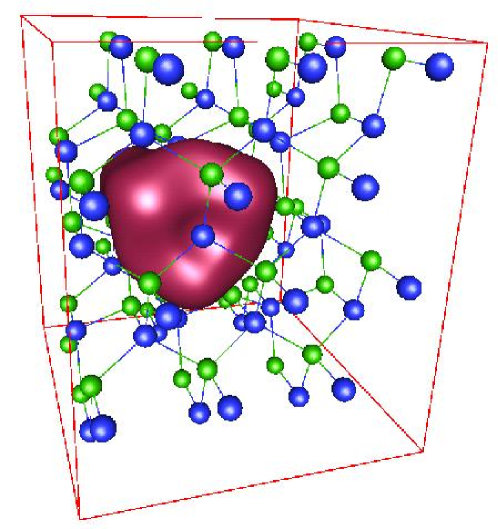
b)

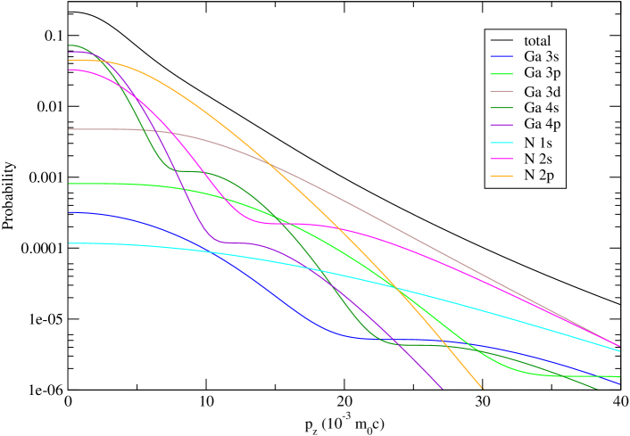
Figure 5. a) An isosurface of the positron wave function localized at a Ga vacancy in GaN. The Ga atoms are shown by green and the N atoms by blue spheres. b) The total and decomposed Doppler spectrum for the Ga vacancy in GaN calculated using the MIKA/doppler program. The contributions of the individual orbitals of the Ga and N atoms are shown by colored lines.

The MIKA/doppler program uses the atomic superposition method. One can either use the LDA parametrizations (enhancement factor and correlation potential) by Boroński and Nieminen [125] or the gradient-corrected scheme by Barbiellini et al [128, 129]. However, the atomic superposition method cannot be used for the low-momentum part due to valence electrons. For that purpose self-consistent all-electron valence wavefunctions have to be constructed. For example, we have used the projector augmented-wave (PAW) method implemented in the plane-wave code Vienna Ab initio Simulation Package (VASP) [59, 60, 130, 131, 127]. Recent applications of the real-space solvers of the MIKA package to positron studies include, for example, a study of vacancy-impurity complexes in highly Sb-doped Si [132] in which computational Doppler spectra were used to identify experimentally detected unknown vacancy-type defects and and a study of the effects of positron localization on the Doppler broadening of the annihilation line in the case of Al [133].

Figure 5a shows an example of a positron state calculated for a Ga vacancy in GaN. The corresponding Doppler spectrum calculated with the MIKA/doppler program is shown in Fig. 5b. The figure shows also the decomposed momentum distributions corresponding to annihilations with electrons on different orbitals. Their weights are calculated with Eq. (34).

The MIKA/doppler program also enables one to calculate the forces on ions due to a localized positron within the atomic superposition approximation. These forces can be used together with electron-ion and ion-ion forces calculated with standard methods in order to find the relaxed ionic configuration of a vacancy-type defect at which there is a localized positron [127].

5.4. All-electron finite-element calculations

             

             

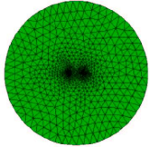
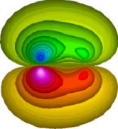
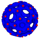
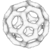
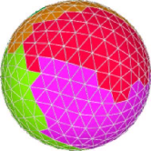
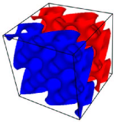
Figure 6. Some electronic structure calculations using Elmer. All-electron calculations for the molecules CO and C₆₀ were performed. Implementation of periodic boundary conditions was tested in the case of bulk silicon. See also the text.

Although the main emphasis of the MIKA-project has been thus far on the support and development of the MIKA-package, which is based on finite-differences, it has been interesting to perform some simple test calculations using the general purpose finite-element package Elmer (Sec. 4.4). Some of these calculations have been already reported in Ref. [80].

Fig. 6 illustrates three test cases. As the first self-consistent calculation within the local-density approximation of the density-functional theory using Elmer, an all-electron calculation for the carbon monoxide molecule was performed. The top left panel of Fig. 6 illustrates the main features of the selected finite-element mesh. Since the divergent ($1/r$) potential has to be represented on the mesh, a very fine mesh is used in the immediate neighbourhood of the singularity. The mesh was generated using Netgen [14], consisted of 120 000 quadratic elements and 170 000 node points. Each node point corresponds to one basis function. To solve the Kohn-Sham eigenvalue problem, the Arpack package was utilized, with incomplete LU-factorization [68] as the preconditioner within the computationally expensive inversion part of the shift and invert step of the Lanczos method as discussed in Sec. 3.2.1 and Sec. 3.1.1. The initial guess for the effective potential was the sum of the bare nuclear potentials. We used an ad hoc linear mixing scheme, where the effective potential at each iteration was a linear combination of the input and output potential, with an exponentially decreasing weight for the input potential, resulting in fast convergence once the decay parameters were properly adjusted. In the middle panel of the upper row of Fig. 6 a contour plot of a single-particle wave function provided by the Kohn-Sham scheme is shown. Also larger molecules can be treated using this all-electron scheme within Elmer. The top right panel of Fig. 6 shows a selected orbital from an all-electron calculation of the C₆₀-molecule. The lower left panel illustrates the electron density of C₆₀, obtained from a parallel calculation involving eight processors and $4\times 10^{5}$ degrees of freedom. In this calculation the preconditioner used in the CG-method of the inversion step was a multigrid method. The lower middle panel of Fig. 6 illustrates the partitioning of the mesh that was used – domains with different colours were mapped to different processors with the help of the Metis program [134]. Periodic boundary conditions were implemented within Elmer, and in order to compare the computational efficiency of the RQMG method and the Lanczos method, the Schrödinger equation was solved (i.e. a non-self-consistent calculation was done) in a periodic potential corresponding to bulk silicon using both methods. A uniform grid consisting of 32³ points was used in the 64-atom supercell. The computational efficiencies of the two methods were found to be similar. The lower right panel of Fig. 6 illustrates a selected eigenfunction from this periodic test case.

The calculation on carbon monoxide reported above, originally performed in 2002, was revisited in 2005, taking advantage of the novel mesh generator GiD [135]. This time only 28 000 second order elements (39 000 basis functions) were required. The accuracy of the computation was checked by evaluating the dipole moment of the molecule, which is a well known basis-set sensitive quantity. The result $-0.235D$ was obtained, whereas the basis-set limit for this quantity is $-0.226D$ [136].

There is plenty of room for improvement in the computational efficiency of our Elmer-based solver, and the next steps required seem to be straightforward. Implementing norm-conserving pseudopotentials or PAW, gathering experience on making meshes with higher-order $p$-elements, possibly with the order variable in space (these are now available in Elmer) as well as paying more attention on the choice of the eigenproblem solver and mixing scheme will improve the efficiency considerably.

5.5. Ballistic transport calculations using the Green’s function method

In this section we present calculations of finite element implementation for the transport properties of the nanostructures.

In the DFT the electron density of a system is constructed from eigenfunctions of the single-particle Hamiltonian. For isolated systems, such as molecules or quantum dots, the whole system can be included in the calculation volume. However, this is not possible in general and some approximations have to be done. In the case of bulk materials the systems are treated as infinite by using periodic boundary conditions. In transport problems the nanostructure modeled is connected to two or more leads so that the system size is infinite but does not have periodicity. A solution to this problem is to calculate the electron density from the single-particle Green’s function with the open boundary conditions [137]. This makes finite-size effects small. The Green’s function method has also other useful properties in transport calculations. For example, it is possible to apply a bias voltage across the system and calculate the current through it.

Green’s functions in transport calculations are heavy to calculate numerically which has delayed their first-principles implementations until the recent years. The computational methods have to be chosen carefully. Typically one uses a special basis set, such as atomic orbitals [138, 139], tailored to describe the equilibrium electronic properties of the system in question. Because a systematic error control is not straightforward with atomic orbitals, the development of other types of solvers is well motivated. We have implemented the Green’s function transport formalism using the FEM with $p$-elements up to the fourth order polynomials [140]. The solver has one, two, and three-dimensional versions so that different types of nanostructures can be modeled. The other implementations beyond the atomic-orbitals ones employ an $O(N)$ optimized basis [141], a wavelet basis [142], full-potential linearized augmented plane-waves [143], maximally localized Wannier functions [144], a finite-difference method [145], and a finite-element method fith linear basis functions [146].

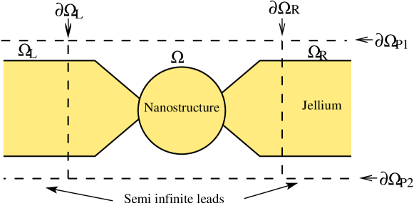
Figure 7. Schematic sketch of modelling a nanostructure.

A brief introduction to the Green’s function method is based on the schematic sketch in Fig. 7. The calculation region is divided into the three parts $\Omega_{R}$, $\Omega$, and $\Omega_{L}$. The nanostructure is located in $\Omega$ and it is connected to the two leads $\Omega_{R}$ and $\Omega_{L}$ using the open boundary conditions on $\partial\Omega_{L/R}$. This means that electrons can travel through the boundaries $\partial\Omega_{L/R}$ without reflection. The system is also open in the sense that during the iterations towards the self-consistent solution the number of electrons in $\Omega$ is not a constant. On the boundaries $\partial\Omega_{P1/P2/P3/P4}$ Dirichlet’s or periodic boundary conditions are applied.

In the Green’s function method the electron density is calculated from the retarded Green’s function $G^{r}$. This requires first the solving of the equation

$$\Big{(}\omega+\frac{1}{2}\nabla^{2}-V_{\rm eff}({\bf r})\Big{)}G^{r}({\bf r},{\bf r}^{\prime};\omega)=\delta({\bf r}-{\bf r}^{\prime}),$$ (36)

where $\omega$ is the electron energy and $V_{\rm eff}$ is the effective potential in the system. The separation between the two solutions $G^{r}$ and $G^{a}$ is made using the boundary conditions. In practice, most of the calculation time is spent in solving the corresponding equation. The calculation of the electron density requires integration over the electron energy so that $G^{r}$ has to be calculated at several energy values. However, when the integration path is moved to the complex plane, the numerical integration does not require many points. Moreover, the integration is easy to parallelize.

In transport calculations we are interested in the electron current. In the Green’s function formulation the current is calculated using the Landauer type of formulation

$$I=\frac{1}{\pi}\int_{-\infty}^{\infty}T(\omega)\left(f_{L}(\omega)-f_{R}(\omega)\right)d\omega.$$ (37)

Note that the above tunneling probability $T(\omega)$ is not the real probability in the sense that it can be larger than unity because it includes the summation over the different conducting channels. A channel can contribute to the conductance by one conductance quantum at maximum. Similarly to the electron density, $T$ is also calculated using the $G^{r}$ function.

In order to use the FEM we first write the equations of the Green’s function method in the so-called variational form. This is how also the numerical form for the open boundary conditions can be derived. The result is analogous to the truncated matrix derivation used, for example, in the case of the finite-difference method [147]. First we take a nicely-behaving arbitrary function $v({\bf r})$ and multiply both sides of Eq. (36) by it. Then we integrate over the calculation domain $\Omega$. We use the properties of the open boundary system and make some manipulations [148], which are shown in detail in Ref. [149]. After this the equation takes the form

$$\int_{\Omega} \Big{\{}-\nabla v({\bf r})\cdot\frac{1}{2}\nabla G^{r}({\bf r,r^{\prime}};\omega)+v({\bf r})\big{[}\omega-V_{\rm eff}({\bf r})\big{]}G^{r}({\bf r,r^{\prime}};\omega)\Big{\}}\,d{\bf r}$$ (38)

$$-\langle\hat{\Sigma}_{L}G^{r},v\rangle-\langle\hat{\Sigma}_{R}G^{r},v\rangle=\,v({\bf r^{\prime}}),$$

where the so-called self-energy operators of the leads have the form

$$\langle\hat{\Sigma}_{L/R}G^{r},v\rangle=$$ (39)

$$\int_{\partial\Omega_{L/R}}\int_{\partial\Omega_{L/R}}\frac{1}{4}G^{r}({\bf r}_{L/R}^{\prime},{\bf r^{\prime}};\omega)\frac{\partial^{2}g_{e}({\bf r}_{L^{\prime}/R^{\prime}},{\bf r}_{L/R};\omega)}{\partial{\bf n}_{L/R}\partial{\bf n}_{L^{\prime}/R^{\prime}}}\,v({\bf r}_{L/R})\,d{\bf r}_{L^{\prime}/R^{\prime}}d{\bf r}_{L/R}.$$

The open boundary conditions of the system are included in the self-energy operators. They are the surface integrals over the open boundaries $\partial\Omega_{L/R}$. The function $g_{e}({\bf r}_{L^{\prime}/R^{\prime}},{\bf r}_{L/R};\omega)$ is the Green’s function of the isolated lead $\Omega_{L/R}$ with the zero boundary condition on the boundary $\partial\Omega_{L/R}$ [148]. In this equation $g_{e}({\bf r}_{L^{\prime}/R^{\prime}},{\bf r}_{L/R};\omega)$ is differentiated with respect to both arguments in the direction of the normal vector ${\bf n}_{L/R}$ on the surface $\partial\Omega_{L/R}$.

The solution for $G^{r}$ can be calculated from 38 by using the finite-element approximation $G^{r}({\bf r,r^{\prime}};\omega)\approx\sum_{i,j=1}^{N}g_{ij}(\omega)\,\phi_{i}({\bf r})\,\phi_{j}({\bf r^{\prime}})$ and choosing $v({\bf r})=\phi_{p}({\bf r})$.

The calculation of the $G^{r}$ function requires inverting of large matrixes. We use a direct sparse solver for this purpose [74]. A direct solver routine requires more computer memory than iterative methods. However, when one has to solve a lot of linear equations with the same coefficient matrix but different left hand sides direct routines are more efficient than iterative ones.

We have used our FEM implementation for modeling of two-dimensional quantum point contacts [150], Na atomic wires [140], and thin HfO₂ layers [140].

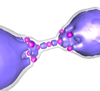
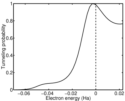
Figure 8. Example of a nanostructure transport problem, i.e., a chain of three Na atoms. The left-hand side shows constant electron density surfaces against the backbone of the Na pseudoatoms (red spheres). The bulk electrodes are described using the jellium background charge. The right-hand side gives the tunneling probability as a function of the electron energy. The energy zero (dashed line) corresponds to the Fermi energy.

5.6. Solution of atomic orbitals using interpolating wavelets

Figure 9. (a) Relative error of the hydrogen 1s orbital eigenvalue, unit of length $u=1.0$. (b) Energy eigenvalues of 2s, 2p, 3s, 3p, 3d, and 4f orbitals of hydrogen with $B=15,20,30,30,30,\;\textrm{and}\;45$, respectively. Ratio of the computed and exact values is shown. Reprinted with permission from T. Höynälänmaa et al., Phys. Rev. E 70, 066701 (2005). Copyright (2005) by the American Physical Society.

Wavelets have been used for solving partial differential equations and the electronic structure, in particular, only recently [151, 152, 44, 153]. Most authors have chosen compactly supported orthonormal wavelets. Daubechies wavelets [154, 153], Meyer wavelets [155], and Mexican hat wavelets [152] have been used. Three of the authors of the present paper performed electronic structure calculations for hydrogen and some many electron atoms with interpolating wavelets [156]. Goedecker and Ivanov used interpolating wavelets to solve the Poisson equation [157].

Orthonormal wavelet families provide useful properties like recursive refinement relations and they lead to fast discrete wavelet transform for multiresolution analysis. Wavelet methods are closely connected to point-grid based methods that also generalize to higher than one dimensions [158, 159]. Lippert et al.  [160] have used interpolating wavelets in point-grid based methods.

Representation of operators in orthonormal wavelet bases has also been studied [161, 162, 163] and we have introduced an algorithm to compute the standard operator form of an arbitrary operator from its nonstandard operator form. Nonstandard operator form decouples different resolution levels, which turns out to be an important aspect for numerical approaches.

Figure 10. (a) Computed total energies for helium, beryllium, neon, magnesium, and argon. Ratio of computed and accurate [164] values is shown. (b) Computed total energies for lithium and sodium. Ratio of computed and accurate [164] values is shown. Reprinted with permission from T. Höynälänmaa et al., Phys. Rev. E 70, 066701 (2005). Copyright (2005) by the American Physical Society.

Due to spherical symmetry of atoms the three dimensional single-particle equation $\hat{H}\psi=\varepsilon\psi$ of the hydrogen-like atoms is separated to the one dimensional radial part and the two dimensional angular part. Exact solutions to the latter are spherical harmonics $Y_{\ell m_{\ell}}$ where $\ell$ and $m_{\ell}$ are the orbital quantum number (angular momentum quantum number) and orbital magnetic quantum numbers, respectively. Writing $R_{n\ell}$ for the radial wavefunction the hydrogen-like orbitals are $\psi_{n\ell m_{\ell}}(r,\theta,\phi)=R_{n\ell}(r)\,Y_{\ell m_{\ell}}(\theta,\phi)$, where $n$ is the principal quantum number. The radial Schrödinger equation for a hydrogen-like atom is

$$\left[-\frac{1}{2}\frac{d^{2}}{dr^{2}}-\frac{Z}{r}+\frac{\ell(\ell+1)}{2r^{2}}\right]P_{n\ell}(r)=\varepsilon_{n\ell}P_{n\ell}(r),$$ (40)

where $Z$ is the atomic number, $\varepsilon_{n\ell}$ are the orbital energies, and $P_{n\ell}(r)=rR_{n\ell}(r)$ are the radial wavefunctions multiplied by $r$. Functions $P_{n\ell}(r)$ are called wavefunctions, too. In general, the radial wavefunction $P_{n\ell}$ has $n-\ell-1$ nodes [165].

The Schrödinger equation $\hat{H}\Psi=E\Psi$ of a many-electron atom leads to Hartree-Fock equations in the central field approximation and with Slater determinant wavefunctions [166, 165, 167]. The Hartree-Fock equations for many-electron atoms are presented e.g. in our previous article [156]. We omit the nondiagonal Lagrange multipliers and HF equations can be written as matrix eigenvalue equations [168]

$${F}_{{i}}{c}_{{i}}=\varepsilon_{{i}}{c}_{{i}}.$$ (41)

The basis sets used for the computations were formed so that there are S type basis functions $\varphi^{k_{\mathrm{min}}}_{-2B},\ldots,\varphi^{k_{\mathrm{min}}}_{2B}$ in resolution level $k_{\mathrm{min}}$ and and D type basis functions $\psi^{k}_{-B},\ldots,\psi^{k}_{B-1}$ for $k=k_{\mathrm{min}},\ldots,k_{\mathrm{min}}+L-2$. Here $L$ is the number of resolution levels and $B$ is a parameter describing the number of basis functions in each resolution level.

Relative error of the hydrogen 1s orbital eigenvalue is plotted in figure 9 (a). Here the computation parameters $L$ and $B$ are varied. In figure 9 (b) the energy eigenvalues for several excited states of hydrogen are plotted. Here the number of resolution levels $L$ is varied. Results for HF computations for closed-shell atoms are presented in figure 10 (a) and for open-shell atoms in figure 10 (b).

To summarize, we have demonstrated that interpolating wavelets can be successfully used to solve the atomic orbitals and the electronic structure of atoms. We were able to systematically increase the accuracy of the calculations by choosing the number of resolution levels and the number of basis functions at each level. This kind of flexibility is an important benefit of wavelets. The numerical results were found to converge to the exact ones as the number of resolution levels increases. However, with a large number of resolution levels the needed computation capacity increases considerably. A noticeable feature in our development for the Hartree-Fock formalism is that all relevent operators can be evaluated analytically.

6. Future developments

In the following we list of our future plans with regard to the further development of software based on each of the three discretization methods. This is done in order to shed light on the motivation behind the work reported in Sec. 5 and to stimulate discussions and collaborations.

6.1. Finite differences

The emphasis on the MIKA-project will be in the development of the finite difference method within the GridPaw-code. The main scientific objective in the near future is the implementation of time-dependent density functional theory (TDDFT) both in the linear response limit and in the real-time domain. These formulations can be used, for example, for the calculation of optical absorption spectra and band gaps of semiconductors and insulators. The real-time formulation is needed for non-linear phenomena such as the electron dynamics under strong femtosecond laser pulses. Recently, a useful survey of time-propagation methods has been publihed by Castro et al. [66].

The time dependent DFT problems are often solved using operator splitting methods. This means that the Laplacian part is transferred to Fourier side with FFT and propagated there, while the potential is exponentiated directly in real space. Mostly second or fourth order splitting schemes are used. This is in fact completely analogous to the diffusion algorithm of Sec. 3.2.4, which can be seen as propagation in imaginary time.

Recently, the so called exponential integrators have turned out to be very effective, especially in parabolic problems [169]. These integrators use the exponential of the linear approximation. The development to hyperbolic systems, as TDDFT, is under active study. An interesting option for equation $x^{\prime}=f(x)$ is, for example, the following exponential explicit midpoint rule [170]

$$x^{k+1}=x^{k}+e^{hH}(x^{k-1}-x^{k})+2h\,\phi(hH)\,f(x^{k})\ ,$$ (42)

where $H$ is an approximation of $f^{\prime}(x^{k})$ and $\phi(z)=(e^{z}-1)/z$. This produces a time reversible propagator, with good norm and energy preservation properties. Computations of $e^{hH}v$ will be done using Krylov subspace techniques. Efficient preconditioning for these, is under active study. Also variants of the use of Magnus expansions for the exponential seem to be promising [171].

The search for new, better exchange correlation functionals is an ever-growing quest within DFT. One problem in the standard LDA and GGA functionals is that part of the self-interaction contribution of the Hartree- and Coulomb-potentials remain in the total energy functional. One result of this remaining self-interaction contribution is that in finite systems the potential decays exponentially instead of the correct $1/r$ behaviour. In contrast to the LDA, the Hartree-Fock scheme is self-interaction free and has the correct asymptotic behaviour. One approach to improve from the LDA is the so-called optimized potential method (OPM) where a multiplicative potential is constructed from a Hartree-Fock-like exchange energy functional [172, 173]. This potential, which depends explicitly on the Kohn-Sham orbitals, has to solved from a complicated integral equation. We are going to implement this exact-exchange scheme by using the KLI-approximation [174] for the OPM integral equation.

6.2. Finite element methods

Even though finite differences methods are currently the most well established in the context of the electronic structure calculations, it is clear that FE-methods could provide certain advantages. Thus, further assessment of the feasibility of FE methods in electronic structure calculations is one of the objectives of the current MIKA-project

In this section we briefly summarize what we already have and what is still missing. All-electron ground-state calculations for molecules can be performed today with Elmer, as described in Sec. 5.4. With the commercial mesh generator GiD significant reduction in the number of second order basis functions for a high quality computation of the carbon monoxide molecule was observed (Sec. 5.4) in comparison with the 2002 version of Netgen. Interestingly, both of these discretizations yielded smaller matrix problems than a state-of-the-art finite-difference pseudopotential approach (see Sec. 7.2), and also computations of larger molecules (C₆₀) were shown to be feasible. Periodic boundary conditions have been implemented. Further improvements of efficiency utilization of $hp$-elements, pseudopotentials (or PAW) and fine-tuning of the eigenproblem solver and mixing scheme. On the other hand, if we aim at an efficient method for real-time TDDFT calculations, the performance (in terms of cpu-time) of the eigenproblem solver and mixing scheme becomes less critical, whereas the reduction of the size of the Hamiltonian matrix becomes even more important.

An alternative route to a general purpose FE-package may be provided by the code described in Sec. 5.5. This program already includes an implementation of norm-conserving pseudopotentials. This implementation can possibly be adapted to Elmer, or an eigenproblem solver can be added into the transport code.

The question of the feasibity of molecular dynamics with an unstructured nonuniform FE-mesh is often raised. The FE-community provides the following suggestion, based on experience in other fields: each atom is attached to the mesh, and the mesh is considered to be made of ”rubber”. As the atom moves, the mesh moves along, but only within a finite range, and towards the boundary of the range the mesh moves less. Therefore, the basis functions are indeed functions of atomic coordinates and Pulay forces occur. If the atoms move over large distances, they may ”tear the mesh apart” locally, by making certain corners of tetrahedra too sharp. In this case local remeshing is applied. In this context, it should be also pointed out that successful molecular dynamics simulations using structured nonuniform finite-element meshes (in so called adaptive coordinates) have been performed already by Tsuchida [20]. As a final remark we add, that the possibility to use nonuniform unstructured meshes within FEM is a very useful, but optional feature. It is also possible to work with uniform meshes, and indeed implementation of molecular dynamics is easier in that case. Even a uniform high-order FE-mesh is expected to be more efficient than a uniform FD-grid – at least in the simplest case where no interpolation tricks are applied on the FD-side – in terms of the required number of basis functions (or grid points) for a given accuracy.

6.3. Wavelet package

The wavelet based approximation scheme is still quite recent computational tool in electronic structure calculations even though it has shown to be very successful in other applications in science and engineering. Its use so far has been mostly restricted to cases which reduce to one-dimensional problems and whose solutions by other methods are well known in the literature. However, a promising recent development should be noticed in this context [175].

In near future we will continue the investigation to which extent the wavelet method can speed up the computation of the atomic orbitals. Especially we will study two and three-dimensional problems. We are currently investigating the use of interpolating tensor product wavelets for these calculations. Special kind of nonseparable wavelets may be better for this purpose. They allow achieving the full benefit of the fast evaluation of the discrete wavelet transform. Also the methods will be compared with the more traditional solution methods.

7. Discussion

In this section we compare the different methods of discretization from various points of view. The discussion is biased towards comparing the FE and FD methods to each other, the wavelet approach is not equally well represented here due to the lack of experience on wavelets of the authors of the present section.

In Sec. 7.1 we discuss the similarities and differences of the discretization methods, emphasizing aspects of local refinements, ease of implementation and linear algebra. In Sec. 7.2 a quantitative comparison between the sizes of the resulting matrix problems in a pseudopotential FD method and an all-electron FE-calculation for CO is made. Also some speculation based on FE-results from a transport calculation with pseudopotentials is presented. In Sec. 7.3 we present an awkward transition (in latin: pons asini) from the double grid method of Ono and Hirose [16] to the state-of-the art finite-element method.

7.1. Similarities and differences between the methods of discretization

The three methods for the discretization of the eigenvalue equation considered in this paper have significant similarities but also some differences. The most notable difference is that in the finite-element and the wavelet method a basis set is present whereas the finite-difference method relies on representing functions by their values at grid points in space. This difference has two main consequences.

1. The use of a basis set gives more freedom for constructions with varying spatial resolution. It is also easy to take into account details in geometry and general forms of boundary conditions. On the other hand, one must be able to generate non-uniform meshes conforming to details in geometry in three dimensions.

2. The basis set nature of the finite-element and the wavelet methods allows the use of variational arguments in the development of the method. This decreases the regularity requirements imposed on the solution and leads to a simpler error analysis.

Let us discuss the question of varying spatial resolution a bit more closely. In the finite-difference context the main approach is the method of adaptive coordinates [4, 79, 176] This method involves a mapping from a regular grid in three-dimensional parameter-space to a curvilinear coordinate system in real-space. This approach obviously has some limitations with regard to the ratio of smallest and largest local grid-spacing, and at least cannot be regarded as a promising approach for all-electron calculations of heavy elements. Special care has to be exercised in order to obtain symmetric finite-difference matrix representation of the Laplacian in adaptive coordinates [79, 5]. Nonsymmetric matrices would render standard iterative methods from linear algebra, such as the conjugate gradient method, or Lanczos method for matrix exponentiation required in time-propagation schemes [66] unreliable. On the finite-element side, an implementation of adaptive coordinates has been introduced as well [6], but the pure FE-approach involves instead general unstructured meshes consisting of elements of various, often tetrahedral, shapes (see Sec. 2.3). This approach allows greater spatial variations in the element size, granting accurate all-electron calculations with problem sizes much smaller than the corresponding FD-grids in pseudopotential calculations (see Sec. 7.2). The resulting matrices ($H,S,A$) in finite-element methods are symmetric by construction. For the sake of completeness, we mention that another approach, namely that of composite grids [177, 178], has been introduced in the context of finite-differences for varying spatial resolution. In this method, local patches of finer grids are applied. In the wavelet approach, local refinements are applied in a similar way [159].

From an algorithmical point of view the finite-difference psedopotential method with uniform grid and trapetsoid rule (Eq. 6) seems to be the simplest one from the first outlook. The resulting matrices are well-structured with a regular hierarchy. On the other hand, in the basis set methods each element of the mesh can be processed using the same algorithm as long as all the elements are affine images of some basic reference element. This is especially easy in the wavelet method where the basis functions are obtained via a simple scaling methodology. When implementing a finite-element code, it is possible and important to reuse large parts of the general purpose finite-element codes which are freely available to the general public, such as those of Refs. [15, 14]. When basic routines are recycled, the implementation of an FE-approach becomes very simple as well.

From the viewpoint of linear algebra all the methods have rather similar characteristics They all result in sparse matrices whose condition number is governed by the underlying differential operator. They all allow the use of multilevel and domain decomposition methods with effective preconditioners. The major differences in favor of FD appear only for very large systems with several hundred million degrees of freedom when the well-structured nature of the finite-difference grid makes it possible to apply the matrix on a vector in an iterative scheme without explicitly storing it at any stage of the computation. In our FE-examples presented below, where second and fourth order tetrahedral meshes were considered, the storage of the necessary matrices (not counting pseudotentials as dense blocks) required memory equivalent to the storage of the order of one hundred eigenfunctions. This remains the case for larger systems as well, thus the relative extra storage becomes increasingly insignificant as larger systems are addressed, in the typical applications where a set of all occupied (and possibly some unoccupied) states need to be calculated.

7.2. Quantitative comparisons

It is difficult to make objective comparisons between two different discretization methods based on two different implementations as computer programs. There are very many parameters that affect the efficiency of the programs, and in the end, the user is only interested in the cpu-time required for a calculation with given accuracy. An objective comparison of the efficiencies of the discretization step, however, has to focus on the size of the matrix problem produced, rather than on the cpu-time spent by the entire calculation (unless exactly the same implementation is used for the solution of the resulting matrix problem). The cpu-time spent at the solution step then depends, apart from the size of the matrix problem, also on the implementation details and on the algorithms chosen for the eigenproblem, linear systems of equations, and mixing.

The dipole-moment of the carbon monoxide molecule is a well known basis-set sensitive quantity. Even with the high-order FD-method and the straightforward trapetsoid rule of Eq. 6, a rather small grid spacing of 0.2 a.u. is required for a converged result (with a tolerance of $0.01D$) when norm conserving Trollier-Martins (TM) psedopotentials are used [179]. When the computational volume is a sphere of radius 10 a.u., this results in 520 000 grid points. A smaller sphere results in loss of accuracy for the value of the dipole moment. Interestingly, the number of degrees of freedom in this calculation is greater than the number of the 39 000 quadratic basis functions in the all-electron FE-calculation within a sphere of radius 20 a.u., reported in Sec. 5.4. There is no essential difference in the average number of nonzero matrix elements per row in the two calculations. This number was 42 in the FD case and 55 in the FE case.

In Sec 5.5 and Ref. [140] a thin HfO₂ layer was modelled with Green’s functions, TM pseudopotentials and fourth order $p$-elements. The unit cell, periodic in two dimensions, consisted of 85 atoms, with dimensions of $27\times 21\times 21a_{0}^{3}$. 28 000 basis functions were considered sufficient for converged results. This was a transport calculation where Green’s functions were evaluated, and we have no experience on the equivalent calculations using FD-methods. However, extrapolating from experience with Kohn-Sham-equations, and also in light of the previous example it is plausible to conclude that the grid spacing of 0.75 a.u., that would result in 28 000 grid points in this case, can hardly give reliable results.

7.3. Generalizing the double grid method

At the end of Sec. 2.1 we recognized, that the double-grid method of Ono and Hirose [16] in fact amounts to computing the matrix elements of the pseudopotential operator in a special basis set arising from the polynomial interpolation used. We repeat here the formula for the matrix elements of the pseudopotential operator

$$V^{\rm nl}_{ijk,i^{\prime}j^{\prime}k^{\prime}}=\sum_{l}c_{l}\tilde{x}_{lijk}\tilde{x}_{li^{\prime}j^{\prime}k^{\prime}}=\int\phi_{ijk}({\mathbf{r}})\hat{V}^{\rm nl}\phi_{i^{\prime}j^{\prime}k^{\prime}}({\mathbf{r}})d{\mathbf{r}},$$ (43)

where the required integrals are approximated by a trapetsoid rule on a fine uniform grid. For the sake of consistency, it is tempting to ask if not the same idea could be applied to the entire hamiltonian $H$, i.e., replace it with a discrete version

$$H_{ijk,i^{\prime}j^{\prime}k}=\int\phi_{ijk}({\mathbf{r}})\hat{H}\phi_{i^{\prime}j^{\prime}k^{\prime}}({\mathbf{r}})d{\mathbf{r}}.$$ (44)

Indeed, this can be done, but then we must keep in mind that the basis set of ${\phi_{ijk}}$’s is not orthonormal, but their overlap matrix

$$S_{ijk,i^{\prime}j^{\prime}k}=\int\phi_{ijk}({\mathbf{r}})\phi_{i^{\prime}j^{\prime}k^{\prime}}({\mathbf{r}})d{\mathbf{r}}.$$ (45)

also enters the formalism, and we end up with the matrix equation $Hc=\varepsilon Sc$ for the unknown coefficients in the expansion

$$\psi({\mathbf{r}})=\sum_{ijk}c_{ijk}\phi_{ijk}({\mathbf{r}}).$$ (46)

The procedure outlined above can be recognized as a variational method of Sec. 2.2 with the basis set of $\phi_{ijk}$’s spanning both the trial and test spaces. Thus the double grid method itself is somewhere between the straightforward FD-scheme of Eqs (5,6) and the finite-element method. Some similarities with the present considerations can be seen in the approach based on the “Galerkin transfer”, outlined in Refs. [64, 65], where a discretization on a grid was obtained from an FD-discretization on an auxiliary finer grid, taking advantage of the prolongator and restrictor operarors from the multigrid formalism. The present approach can be seen as a limiting case, where the fine grid is replaced by continuous space.

We add two more comments. i) When numerically evaluating integrals such as Eqs. (8, 44, 45) the trapetsoid rule with uniform sampling is not the most efficient method. The integrands have support only within an orthorhombic volume, and very efficient numerical cubature formulas within such standard volumes are well known [182]. ii) Although the thought experiment above gave a continuous path from the double-grid method to the FE-method with a basis consisting of the functions $\phi_{ijk}$, we do not suggest extending this basis set to very high order polynomials as it may result in matrices with high condition number.

Other bases of low order polynomial product form are e.g. the ”blip”-function basis (in the special case of $k=0$) of Hernandez and Gillan [11] as well as the polynomial product basis of Tsuchida and Tsukada [183]. The nonseparable cubic ”serendipity” element [37] gives rise to a useful basis set which is no longer of product form, but still is associated with a simple uniform grid structure. To complete our awkward transition from the double grid method to the state-of the art FE-methods [34, 35, 36], we repeat here that the tetrahedral $p$-element basis [39, 140] discussed in Sec. 2.3.1 associated with a good mesh generator such as the rapidly developing open source Netgen-package [14] grants us, in principle, with complete flexibility in locally selecting the polynomial order $p$ as well as the element size $h$.

8. Summary

In this paper we have discussed our efforts to develop systematic real-space methods as alternatives to the standard plane-wave and atom-centered basis function methods. We aim at a general purpose infrastructure for electronic structure calculations based on the Kohn-Sham density-functional theory [2, 1] and its time-dependent generalization [3]. Our first line of work is the MIKA-project. In its early stages, this project has been rather tightly bound to the finite-difference method, the Rayleigh-quotient multigrid method, and the MIKA program package. In the near future the main development effort is directed to the implementation of software tools for time-dependent density-functional theory within the GridPaw-code [97]. It is based on a different implementation of the FD method. Its attractive feature is a successful FD-implementation of the Projector Augmented Wave method, originally developed in the plane-wave context, which allows the use of relatively coarse uniform FD-grids for the accurate description of a wide range of elements.

The second theme of this paper has been the promotion of the applications of FE methods within electronic structure calculations. This work extends the scope of the MIKA project. Nowadays, there are general-purpose open-source FE-packages available [14, 15], that are extremely well suited as starting points for the development of solvers for the Kohn-Sham equations. Thus the argument that implementation of FE-methods for electronic structure problems is more difficult than that of the FD-methods has to be reconsidered. We have compared a very preliminary all-electron example calculation for the carbon monoxide molecule with a state-of-the-art pseudopotential FD-calculation, in terms of the size of the matrix problem and seen that the spatially adaptive FE-discretization yields a matrix problem which is more than an order of magnitude smaller. Further reductions in the size of the problem are expected when pseudopotentials or the PAW method is implemented, and/or full advantage is taken of $hp$-FEM methods, where spatial variations in the order $p$ of the piecewise polynomial basis functions are allowed simultaneously with variations in the element size $h$.

Reductions in the CPU-time required by the finite-element ground-state computations may also be available via a careful selection of the eigenproblem solver and mixing scheme. However, as the ultimate goal is to utilize also the FE-approach in real-time propagation within TDDFT, the optimal performance of the ground state solver is of secondary importance (as long as it delivers highly accurate results – this may be critical for the stability of the time propagation – and as it is reliable in the sense that not too much labour of the users needs to be invested in obtaining a convergent ground state calculation) since the time propagation will always consume the dominant part of the cpu-time. The reduction of the size of the Hamiltonian matrix is directly relevant also for the performance of time propagation. From a somewhat more philosophical point of view, we have contemplated on the now popular double grid method due to Ono and Hirose [16], and seen it as the first step in a gradual transformation from the FD-method to the FE-method.

The third line of work discussed in this paper is the development of a program package based on the wavelet approach. This effort is still at a very preliminary stage (thus far only spherically symmetric, computationally one-dimensional results have been reported), and it has been included here mainly with the dual aim of increasing the level of wavelet awareness among the authors of the present paper and of stimulating discussions with the various wavelet specialists. Based on the current results, it is obvious that our wavelet package has not yet reached a level of maturity comparable to that of the FD and FE packages. Thus we will base our TDDFT developments on either one, or both, of these two methods.

T. T. would like to thank the organizers (E. Artacho, E. Hernandez and T. Beck) of the wonderful CECAM-workshop “State of the art developments and perspectives of real-space electronic structure techniques in condended matter and molecular physics”, that took place in Lyon in June 2005. The discussions in the workshop gave the necessary motivation to assemble this paper. The authors are grateful to the advisory board of the MIKA-project for encouragement and discussions during the process of writing this paper. Members of the advisory board that are not also authors of this paper are K. W. Jacobsen (CAMP and CSC), R. M. Nieminen (COMP) and H. Häkkinen (ACQD). E. Krotscheck and M. Aichinger are acknowledged for their collaboration related to the response iteration scheme (see. preamble of Sec. 3, Sec. 5.1 and Sec. 5.2). We are grateful to L. Kronik, M. Johansson and D. Sundholm for useful discussions on the dipole moment of carbon monoxide (see Sec. 7.2). Thanks to J. J. Mortensen and A. Foster for comments on the manuscript during the process of its preparation. T. T., J. E. and T. H. acknowledge financial support from the Finnish technology agency TEKES. The work of E. R. was partially supported by the Austrian Science Fund FWF under project P15083-N08. T. T. is grateful for financial support from the Magnus Ehrnrooth foundation.

References

- [1] W. Kohn and L. J. Sham. Phys. Rev. 140, A1133 (1965).
- [2] P. Hohenberg and W. Kohn. Phys. Rev. 136, B864 (1964).
- [3] E. Runge and E. K. U. Gross. Phys. Rev. Lett. 52, 997 (1984).
- [4] U. V. Waghmare, H. Kim, I. J. Park, N. Modine, P. Maragakis, and E. Kaxiras. Comp. Phys. Comm. 137, 341 (2001).
- [5] A. Castro. Private communication (2005).
- [6] E. Tsuchida and M. Tsukada. J. Phys. Soc. Jap. 67, 3844 (1998).
- [7] F. Gygi. Europhys. Lett. 19, 617 (1992).
- [8] F. Gygi. Phys. Rev. B 48, 11692 (1993).
- [9] P. Blöchl. Phys. Rev. B 50, 17953 (1994).
- [10] P. Blöchl, C. J. Först, and J. Schimpl. Bull. Mater. Sci 26, 33 (2003).
- [11] E. Hernández and M. J. Gillan. Phys. Rev. B 55, 13485 (1997).
- [12] C.-K. Skylaris, A. A. Mostofi, P. D. Haynes, O. Dieguez, and M. C. Payne. Phys. Rev. B 66, 035119 (2002).
- [13] J.-L. Fattebert and J. Bernholc. Phys. Rev. B 62, 1713 (2000).
- [14] Three-dimensional mesh generator Netgen, see http://www.hpfem.jku.at/netgen/index.html.
- [15] Elmer – Finite element software for multiphysical problems, see http://www.csc.fi/elmer.
- [16] T. Ono and K. Hirose. Phys. Rev. Lett. 82, 5016 (1999).
- [17] J. M. Soler, E. Artacho, J. D. Gale, A. Garc a, J. Junquera, P. Ordej n, and D. S nchez-Portal. J. Phys. : Condens. Matter 14, 2745 (2002).
- [18] R. Car and M. Parrinello. Phys. Rev. Lett. 55, 2471 (1985).
- [19] R. N. Barnett and U. Landman. Phys. Rev. B 48, 2081 (1993).
- [20] E. Tsuchida. J. Chem. Phys. 121, 4740 (2004).
- [21] R. Schmid. J. Comput. Chem. 25, 799 (2004).
- [22] L. Kleinman and D. Bylander. Phys. Rev. Lett. 48, 1425 (1982).
- [23] Y. Liu, D. A. Yarne, and M. E. Tuckerman. Phys. Rev. B 68, 125110 (2003).
- [24] D. Baye, M. Hesse, and M. Vincke. Phys. Rev. E 65, 026701 (2002).
- [25] J. Kobus, L. Laaksonen, and D. Sundholm. Comp. Phys. Comm. 98, 346 (1996).
- [26] A. D. Becke. Phys. Rev. A 33, 2786 (1986).
- [27] A. D. Becke. J. Chem. Phys. 88, 2547 (1988).
- [28] M. Springer. Phys. Rev. B 58, 1939 (1998).
- [29] E. L. Briggs, D. J. Sullivan, and J. Bernholc. Phys. Rev. B 52, R5471 (1995).
- [30] L. Collatz. The numerical treatment of differential equations (Springer-Verlag, Berlin, 1960).
- [31] M. Heiskanen. unpublished (1998).
- [32] J. R. Chelikowsky, N. Troullier, K. Wu, and Y. Saad. Phys. Rev. B 50, 11355 (1994).
- [33] F. Nogueira, A. Castro, and M. Marques. In A Primer in Density Functional Theory, edited by C. Fiolhais, F. Nogueira, and M. Marques (Springer-Verlag, Heidelberg, 2003), pp. 218–256.
- [34] D. Braess. Finite Elements (Cambridge University Press, Cambridge, 1997).
- [35] P. G. Ciarlet and J. L. Lions (editors). Finite Element Methods, volume II of Handbook of Numerical Analysis (North-Holland, Amsterdam, 1991).
- [36] B. Szabo and I. Babuska. Finite Element Analysis (John Wiley & Sons, Inc., New York, 1991).
- [37] J. E. Pask and P. A. Sterne. Modelling Simul. Mater. Sci. Eng. 13, R71 (2005).
-
[38]
Two-dimensional mesh generator Easymesh,
see http://www-dinma.univ.trieste.it/nirftc/research/easymesh/Default.htm. - [39] M. Ainsworth and J. Coyle. Int. J. Numer. Meth. Eng. 58, 2103 (2003).
- [40] R. Stevenson. SIAM J. Numer. Anal. 41, 1074 (2003).
- [41] S. Dahlke, W. Dahmen, and K. Urban. SIAM J. Numer. Anal. 40, 1230 (2002).
- [42] W. Dahmen. Acta Numerica 6, 55 (1997).
- [43] M. Lindemann. Approximation properties of non-separable wavelet bases with isotropic scaling matrices. Ph.D. dissertation, Universität Bremen (2005).
- [44] S. Goedecker. Wavelets and their application for the solution of partial differential equations in physics (Presses Polytechniques et Universitaires Romandes, 1998).
- [45] C. K. Chui and C. Li. SIAM J. Math. Anal. 27, 865 (1996).
- [46] D. L. Donoho. Interpolating wavelet transform. Technical report, Dept. of Statistics Stanford Univ. (1992).
- [47] I. Daubechies. Ten Lectures on Wavelets, volume 61 of CBMS-NSF regional conference series in applied mathematics (SIAM, 1992).
- [48] G. H. Golub and C. F. V. Loan. Matrix Computations (The Johns Hopkins University Press, London, 1989), second edition.
- [49] J. Dongarra. In Templates for the solution of Algrebraic Eigenvalue Problems: A Practical Guide, edited by Z. Bai, J. Demmel, J. Dongarra, A. Ruhe, and H. van der Vorst (SIAM, Philadelphia, 2000), p. 372.
- [50] Lapack, Linear Algebra PACKage, see http://www.netlib.org/lapack.
-
[51]
A basic tool-kit for sparse matrix computations Sparskit,
see http://www-users.cs.umn.edu/ saad/software/SPARSKIT/sparskit.html. - [52] A. Brandt. Math. Comput. 31, 333 (1977).
- [53] A. Brandt, S. F. McCormick, and J. W. Ruge. SIAM J. Sci. Comput. (USA) 4, 244 (1983).
- [54] J. Wang and T. L. Beck. J. Chem. Phys. 112, 9223 (2000).
- [55] N. Wijesekera, G. Feng, and T. L. Beck. J. Theor. Comput. Chem. 2, 553 (2003).
- [56] S. Costiner and S. Ta’asan. Phys. Rev. E 52, 1181 (1995).
- [57] E. L. Briggs, D. J. Sullivan, and J. Bernholc. Phys. Rev. B 54, 14362 (1996).
- [58] M. C. Payne, M. P. Teter, D. C. Allan, T. A. Arias, and J. D. Joannopoulos. Rev. Mod. Phys. 64, 1045 (1992).
- [59] G. Kresse and J. Furthmüller. Phys. Rev. B 54, 11169 (1996).
- [60] G. Kresse and J. Furthmüller. Comp. Mat. Sci. 6, 15 (1996).
- [61] D. R. Bowler and M. J. Gillan. Chem. Phys. Lett. 325, 473 (2000).
- [62] J.Auer and E. Krotscheck. Comp. Phys. Comm. 118, 139 (1999).
- [63] J. Auer and E. Krotscheck. Comp. Phys. Comm. 151, 265 (2003).
- [64] T. Torsti, V. Lindberg, I. Makkonen, E. Ogando, E. Räsänen, H. Saarikoski, M. J. Puska, and R. M. Nieminen. Newsletter 65, 105 (2004).
- [65] T. Torsti, V. Lindberg, I. Makkonen, E. Ogando, E. Räsänen, H. Saarikoski, M. J. Puska, and R. M. Nieminen. Handbook of Theoretical and Computational nanotechnology (2006).
- [66] A. Castro, M. A. L. Marques, and A. Rubio. J. Chem. Phys. 121, 3425 (2004).
- [67] H. A. van der Vorst. Iterative Krylov Methods for large linear systems (Cambridge University Press, 2003).
- [68] H. C. Elman. Math. Comput. 47, 191 (1986).
- [69] W. L. Briggs, V. E. Henson, and S. F. McCormick. A Multigrid Tutorial, Second Edition (SIAM, 2000).
- [70] W. Hackbush. Multi-Grid Methods and Applications (Springer-Verlag, Berlin, 1985).
- [71] P. Wesseling. An Introduction to Multigrid Methods (John Wiley & Sons, Inc., New York, 1992).
- [72] I. S. Duff. Comp. Phys. Comm. 97, 45 (1996).
- [73] J. K. Reid and I. S. Duff. ACM Trans. on Math. Software 9, 302 (1983).
- [74] The Harwell Subroutine Library, see http://www.cse.clrc.ac.uk/nag/hsl/.
- [75] T. A. Davis. ACM Trans. Math. Software 30, 353 (2004).
- [76] A. Gupta. IBM Research Report, RC 21886, 98462 (2000).
- [77] Y. Saad. Numerical Methods for Large Eigenvalue Problems (Manchester University Press, Manchester, 1992).
- [78] L.-W. Wang and A. Zunger. Comp. Mat. Sci 2, 326 (1994).
- [79] N. A. Modine, G. Zumbach, and E. Kaxiras. Phys. Rev. B 55, 10289 (1997).
- [80] T. Torsti. Real-Space Electronic Structure Calculations for Nanoscale Systems. Ph.D. dissertation, Helsinki University of Technology (2003). Http://lib.hut.fi/Diss/2003/isbn9512264706/.
- [81] A. Stathopoulos and S. Ögüt and Y. Saad and J. Chelikowsky and H. Kim. Comput. Sci. Eng. 2, 19 (2000).
- [82] A. Knyazev. Siam. J. Sci. Comput. 23, 517 (2001).
- [83] A. Knyazev and K. Neymeyr. El. Trans. Numer. Anal. 15, 38 (2003).
- [84] M. E. Casida. In Recent Advances in Density Functional Methods, Part I, edited by D. P. Chong (Singapore, 1995), p. 155.
- [85] C. Jamorski, M. E. Casida, and D. R. Salahub. J. Chem. Phys. 104, 5134 (1996).
- [86] E. R. Davidson. J. Comp. Phys. 17, 87 (1975).
- [87] E. R. Davidson. Computers in Physics 7, 519 (1993).
- [88] S. J. A. Gisbergen, J. G. Snijders, and E. J. Baerends. Comp. Phys. Comm. 118, 119 (1999).
- [89] R. E. Stratman, G. E. Scuseria, and M. J. Frisch. J. Chem. Phys. 109, 8218 (1998).
- [90] W. R. Burdick, Y. Saad, L. Kronik, I. Vasiliev, M. Jain, and J. R. Chelikowsky. Comp. Phys. Comm. 156, 22 (2003).
- [91] The ScaLapack project, see http://www.netlib.org/scalapack.
- [92] Arpack – Arnoldi package, see http://www.caam.rice.edu/software/ARPACK/.
- [93] M. Heiskanen, T. Torsti, M. Puska, and R. Nieminen. Phys. Rev. B 63, 245106 (2001).
- [94] T. Torsti, M. Heiskanen, M. Puska, and R. Nieminen. Int. J. Quantum Chem. 91, 171 (2003).
- [95] J. Mandel and S. McCormick. J. Comput. Phys. 80, 442 (1989).
- [96] D. M. Wood and A. Zunger. J. Phys. A 18, 1343 (1985).
- [97] J. J. Mortensen, L. B. Hansen, and K. W. Jacobsen. Phys. Rev. B 71, 035109 (2005).
- [98] P. Pulay. Chem. Phys. Lett. 73, 393 (1980).
- [99] P. Pulay. J. Comp. Chem. 3, 556 (1982).
- [100] J. Auer, E. Krotscheck, and S. A. Chin. J. Chem. Phys. 115, 6841 (2001).
- [101] M. Aichinger and E. Krotscheck. Comp. Mater. Sci. 34, 188 (2005).
- [102] M. Aichinger, S. A. Chin, and E. Krotscheck. Comp. Phys. Comm. 171, 197 (2005).
- [103] P. Havu. Modeling of Electronic Transport in Nanostructures. Ph.D. dissertation, Helsinki University of Technology (2005). Http://lib.tkk.fi/Diss/2005/isbn9512278596/.
- [104] For a review, see, e.g., L. P. Kouwenhoven, D. G. Austing, and S. Tarucha, Rep. Prog. Phys. 64, 701 (2001); S. M. Reimann and M. Manninen, Rev. Mod. Phys. 74, 1283 (2002).
- [105] H. Saarikoski, E. Räsänen, S. Siljamäki, A. Harju, M. J. Puska, and R. M. Nieminen. Phys. Rev. B 67, 205327 (2003).
- [106] M. Aichinger and E. Räsänen. Phys. Rev. B 71, 165302 (2005).
- [107] E. Räsänen and M. Aichinger. Phys. Rev. B 72, 045352 (2005).
- [108] U. Sivan, R. Berkovits, Y. Aloni, O. Prus, A. Auerbach, and G. Ben-Yoseph. Phys. Rev. Lett. 77, 1123 (1996).
- [109] S. R. Patel, S. M. Cronenwett, D. R. Stewart, A. G. Huibers, C. M. Marcus, C. I. Duruoz, J. S. Harris, K. Campman, and A. C. Gossard. Phys. Rev. Lett. 80, 4522 (1998).
- [110] K. Hirose, F. Zhou, and N. S. Wingreen. Phys. Rev. B 63, 75301 (2001).
- [111] H. Jiang, D. Ullmo, W. Yang, and H. U. Baranger. Phys. Rev. B 69, 235326 (2004).
- [112] H. Saarikoski, A. Harju, M. J. Puska, and R. M. Nieminen. Phys. Rev. Lett. 93, 116802 (2004).
- [113] H. Saarikoski, S. M. Reimann, E. Räsänen, A. Harju, and M. J. Puska. Phys. Rev. B 71, 035421 (2005).
- [114] H. Saarikoski and A. Harju. Phys. Rev. Lett. 94, 246803 (2005).
- [115] E. Räsänen, H. Saarikoski, A. Harju, M. J. Puska, Y. Yu, and S. M. Reimann. To be published (cond-mat/0509660).
- [116] A. Harju, H. Saarikoski, and E. Räsänen. To be published.
- [117] T. Chakraborty and P. Pietiläinen. The Quantum Hall Effects: Fractional and Integral (Springer-Verlag, Berlin, 1995).
- [118] T. H. Oosterkamp, J. W. Janssen, L. P. Kouwenhoven, D. G. Austing, T. Honda, and S. Tarucha. Phys. Rev. Lett. 82, 2931 (1999).
- [119] M. P. Schwarz, D. Grundler, C. Heyn, D. Heitmann, D. Reuter, and A. Wieck. Phys. Rev. B 68, 245315 (2003).
- [120] M. Manninen, S. M. Reimann, M. Koskinen, Y. Yu, and M. Toreblad. Phys. Rev. Lett 94, 106405 (2005).
- [121] E. Chulkov, V. M. Silkin, and P. M. Echenique. Surf.Sci. 437, 330 (1999).
- [122] I. Sarria, J. Osama, E. Chulkov, J. Pitarke, and P. Echenique. Phys. Rev. B 60, 11795 (1999).
- [123] E. Ogando, N. Zabala, E. V. Chulkov, and M. J. Puska. Phys. Rev. B 71, 205401 (2005).
- [124] G. A. Fiete and E. J. Heller. Rev. Mod. Phys. 75, 993 (2003).
- [125] E. Boroński and R. M. Nieminen. Phys. Rev. B 34, 3820 (1986).
- [126] M. Alatalo, B. Barbiellini, M. Hakala, H. Kauppinen, T. Korhonen, M. J. Puska, K. Saarinen, P. Hautojärvi, and R. M. Nieminen. Phys. Rev. B 54, 2397 (1996).
- [127] I. Makkonen, M. Hakala, and M. J. Puska. Phys. Rev. B 73, 035103 (2006). (cond-mat/0509025).
- [128] B. Barbiellini, M. J. Puska, T. Torsti, and R. M. Nieminen. Phys. Rev. B 51, 7341 (1995).
- [129] B. Barbiellini, M. J. Puska, T. Korhonen, A. Harju, T. Torsti, and R. M. Nieminen. Phys. Rev. B 53, 16201 (1996).
- [130] G. Kresse and D. Joubert. Phys. Rev. B 59, 1758 (1999).
- [131] I. Makkonen, M. Hakala, and M. J. Puska. J. Phys. Chem. Solids 66, 1128 (2005).
- [132] M. Rummukainen, I. Makkonen, V. Ranki, M. J. Puska, K. Saarinen, and H.-J. L. Gossmann. Phys. Rev. Lett. 94, 165501 (2005).
- [133] A. Calloni, A. Dupasquier, R. Ferragut, P. Folegati, M. M. Iglesias, I. Makkonen, and M. J. Puska. Phys. Rev. B 72, 054112 (2005).
- [134] G. Karypis and V. Kumar. SIAM Journal on Scientific Computing 20, 359 (1998).
- [135] The personal pre- and postrocessor GiD, see http://gid.cimne.upc.es/index.html.
- [136] Y. He, J. Gräfenstein, E. Kraka, and D. Cremer. Molecular Physics 98, 1639 (2000).
- [137] S. Datta. Electronic transport in mesoscopic systems (Cambridge University Press, Cambridge, 1995).
- [138] J. Taylor, H. Guo, and J. Wang. Phys. Rev. B 63, 245407 (2001).
- [139] M. Brandbyge, J. Mozos, P. Ordejón, J. L. Taylor, and K. Stokbro. Phys. Rev. B 65, 165401 (2002).
- [140] P. Havu, V. Havu, M. J. Puska, M. H. Hakala, A. S. Foster, and R. M. Nieminen. J. Chem. Phys. (in print); http://arxiv.org/abs/physics/0506159 (2006).
- [141] M. B. Nardelli, J.-L. Fattebert, and J. Bernholc. Phys. Rev. B 64, 245423 (2001).
- [142] K. S. Thygesen, M. V. Bollinger, and K. W. Jacobsen. Phys. Rev. B 67, 115404 (2003).
- [143] D. Wortmann, H. Ishida, and S. Bluegel. Phys. Rev. B 66, 075113 (2002).
- [144] A. Calzolari, N. Marzari, I. Souza, and M. B. Nardelli. Phys. Rev. B 69, 035108 (2004).
- [145] P. A. Khomyakov and G. Brocks. Phys. Rev. B 70, 195402 (2004).
- [146] E. Polizzi and A. N. Ben. J. Comput. Phys. 202, 150 (2005).
- [147] S. Datta and W. Tian. Phys. Rev. B 55, R1914 (1997).
- [148] T. J. R. Hughes. Comput. Methods Appl. Mech Engrg. 127, 387 (1995).
- [149] P. Havu, T. Torsti, M. J. Puska, and R. M. Nieminen. Phys. Rev. B 66, 075401 (2002).
- [150] P. Havu, M. J. Puska, R. M. Nieminen, and V. Havu. Phys. Rev. B 70, 233308 (2004).
- [151] C. J. Tymczak and Xiao-Qian Wang. Phys. Rev. Lett. 78, 3654 (1997).
- [152] K. Cho, T. A. Arias, J. D. Joannopoulos, and P. K. Lam. Phys. Rev. Lett. 71, 1808 (1993).
- [153] Siqing Wei and M. Y. Chou. Phys. Rev. Lett. 76, 2650 (1996).
- [154] P. Fischer and M. Defranceschi. SIAM J. Numer. Anal. 35, 1 (1998).
- [155] K. Yamaguchi and T. Mukoyama. J. Phys. B 29, 4059 (1996).
- [156] T. Höynälänmaa, T. T. Rantala, and K. Ruotsalainen. Phys. Rev. E 70, 066701 (2004).
- [157] S. Goedecker and O. V. Ivanov. Solid State Commun. 105, 665 (1998).
- [158] O. V. Vasilyev, S. Paolucci, and M. Sen. J. Comput. Phys. 120, 33 (1995).
- [159] T. A. Arias. Rev. Mod. Phys. 71, 267 (1999).
- [160] R. A. Lippert, T. A. Arias, and A. Edelman. J. Comput. Phys. 140, 278 (1998).
- [161] G. Beylkin. SIAM J. Numer. Anal. 6, 1716 (1992).
- [162] G. Beylkin and J. M. Keiser. J. Comput. Phys. 132, 233 (1997).
- [163] G. Beylkin, R. Coifman, and V. Rokhlin. Commun. Pure Appl. Math. XLIV, 141 (1991).
- [164] Ch. Froese Fischer. The Hartree-Fock Method for Atoms – A Numerical Approach (John Wiley & Sons, 1977).
- [165] R. D. Cowan. The theory of atomic structure and spectra (University of California Press, 1981).
- [166] P. W. Atkins and R. S. Friedman. Molecular Quantum Mechanics (Oxford University Press, 1997).
- [167] V. Schmidt. Electron Spectrometry of Atoms using Synchrotron Radiation (Cambridge University Press, 1997).
- [168] I. N. Levine. Quantum chemistry (Allyn and Bacon, 1983).
- [169] M. Hochbruck and A. Ostermann. Appl. Numer. Math. 53 (2005).
- [170] M. Hochbruck, C. Lubich, and H. Selhofer. SIAM J. Sci. Comput. 19 (1998).
- [171] M. Hochbruck and C. Lubich. SIAM J. Numer. Anal. 41 (2003).
- [172] V. S. J. Gruenebaum and J. P. Perdew. Phys. Rev. B 26, 4371 (1982).
- [173] D. C. Langreth and M. J. Mehl. Phys. Rev. B 28, 1809 (1983).
- [174] J. B. Krieger, Y. Li, and G. J. Iafrate. Phys. Lett. A 146, 256 (1990).
- [175] I. Daykov, T. Engeness, and T. Arias. Phys. Rev. Lett. 90, 216402 (2003).
- [176] F. Gygi and G. Galli. Phys. Rev. B 52, R2229 (1995).
- [177] T. L. Beck. Rev. Mod. Phys. 72, 1041 (2000).
- [178] E. J. Bylaska, S. R. Kohn, S. B. Baden, A. Edelman, R. Kawai, M. E. G. Ong, and J. H. Weare. In Proceedings of the 7th SIAM Conference on Parallel Processing for Scientific Computing, edited by D. H. Bailey et al. (1995), p. 219.
- [179] L. Kronik. private communication.
- [180] G. te Velde. Numerical Integration and other methodological aspects of bandstructure calculations. Ph.D. dissertation, Vrije Universiteit te Amsterdam (1990).
- [181] G. te Velde and E. J. Baerends. J. Comput. Phys. 99, 84 (1992).
- [182] J. Cools. J. Complexity 19, 445 (2003).
- [183] E. Tsuchida and M. Tsukada. J. Phys. Soc. Japan 67, 3844 (1998).