Spin Transfer Torque for Continuously Variable Magnetization

Abstract

We report quantum and semi-classical calculations of spin current and spin-transfer torque in a free-electron Stoner model for systems where the magnetization varies continuously in one dimension. Analytic results are obtained for an infinite spin spiral and numerical results are obtained for realistic domain wall profiles. The adiabatic limit describes conduction electron spins that follow the sum of the exchange field and an effective, velocity-dependent field produced by the gradient of the magnetization in the wall. Non-adiabatic effects arise for short domain walls but their magnitude decreases exponentially as the wall width increases. Our results cast doubt on the existence of a recently proposed non-adiabatic contribution to the spin-transfer torque due to spin flip scattering.

I Introduction

The use of electric current to control magnetization in nanometer-sized structures is a major theme in the maturing field of spintronics. Fert:2003 An outstanding example is the theoretical prediction of current-induced magnetization precession and switching in single domain multilayers SB and its subsequent experimental confirmation in spin-valve nanopillars. Kiselev:2003 The physics of this spin-transfer effect is that a single domain ferromagnet feels a torque because it absorbs the component of an incident spin current that is polarized transverse to its magnetization. The same idea generalizes to systems with continuously non-uniform magnetization. Berger:1978 ; Bazaliy:1998 This realization has generated a flurry of experimental expt and theoretical work Waintal:2004 ; Tatara:2004 ; Zhang:2004 ; Thiaville:2005 ; Barnes:2005 focused on current-driven motion of domain walls in magnetic thin films.

The experiments cited just above employ Néel-type domain walls with widths $w\approx 100$ nm. This length is very large compared to the characteristic length scales of the processes that determine the local torque.Stiles:2002 ; Zhang:2002 Therefore, it is appropriate to adopt an adiabatic approximation where the spin current is assumed to lie parallel to the local magnetization. Berger:1978 ; Bazaliy:1998 Surprisingly, the adiabatic prediction for the current dependence of the domain wall velocity Berger:1986 ; Tatara:2004 ; Thiaville:2004 agrees very poorly with experiment. This has led theorists Waintal:2004 ; Tatara:2004 ; Zhang:2004 ; Thiaville:2005 ; Barnes:2005 to consider non-adiabatic effects and experimenters Klaui:2005 ; Ravelosona:2005 to study systems with domain wall widths that are much shorter ($w\approx 10$ nm) than those studied previously.

Two groups Zhang:2004 ; Thiaville:2004 have studied the effect on domain wall motion of a distributed spin-transfer torque represented by a sum of gradients of the local magnetization with constant coefficients. For a one-dimensional magnetization ${\bf M}(x)$, the torque function can be written in terms of two vectors perpendicular to the magnetization

$${\bf N}_{\rm st}(x)=c_{1}\partial_{x}\hat{\bf M}+c_{2}\hat{\bf M}\times\partial_{x}\hat{\bf M}.$$ (1)

In general, the coefficients $c_{1}$ and $c_{2}$ are functions of position. The well-established adiabatic piece of the torque is the first term in Eq. (1) with a constant coefficient. Consistent with usage in the literature, we call all deviations from the adiabatic torque non-adiabatic. Any contributions of the second term are then called non-adiabatic. Zhang and Li Zhang:2004 derive a contribution along this second direction in Eq. (1) from a consideration of magnetization relaxation due to spin-flip scattering in the context of an s-d exchange model of a ferromagnet. Berger:1986 ; Zhang:2002 Their arguments lead them to the estimate $c_{2}/c_{1}\approx 0.01$. The authors of Ref. Thiaville:2005, report that a similar value of $c_{2}/c_{1}$ produces agreement with experiment when Eq. (1) is used in micromagnetic simulations.

In this paper, we study the applicability of Eq. (1) to a free-electron Stoner model with one-dimensional magnetization distributions of the form

$${\bf M}(x)=M_{s}\left(\sin\theta\cos\phi,\sin\theta\sin\phi,\cos\theta\right).$$ (2)

In Eq. (2), the polar angle $\theta(x)$ is measured from the positive $z$ axis, $\phi(x)$ is the azimuthal angle in the $x$-$y$ plane, and $M_{s}$ is the saturation magnetization. We begin with the spin current and spin torque for an infinite spin spiral with constant pitch. This system turns out to be perfectly adiabatic; the torque is described by Eq. (1) with $c_{2}=0$. The same is true for realistic domain walls of the sort usually encountered in experiment. Non-adiabatic effects appear only for very narrow walls. In that case, the torque is non-local and cannot be written in the form Eq. (1). The non-adiabatic torque decreases exponentially as the wall width increases for all realistic domain wall profiles. Finally, our analysis casts doubt on the existence of a non-adiabatic contribution to the torque due to spin-flip scattering proposed recently by Zhang and Li.Zhang:2004 .

The remainder of the paper is organized as follows. Section II describes our Stoner model and the methods we use to calculate the spin current and spin-transfer torque. Section III reports our results for an infinite spin spiral and Section IV does the same for one-dimensional domain walls that connect two regions of uniform magnetization. Section V relates these calculations to previous work by others. Section VI discusses the effects of scattering. We summarize our results and offer some conclusions in Section VII. Two appendices provides some technical details omitted in the main body of the paper.

II Model & Methods

The free electron Stoner model provides a first approximation to the electronic structure of an itinerant ferromagnet. The Hamiltonian is

$$H=-{\hbar^{2}\over 2m}\nabla^{2}-\mu\bm{\sigma}\cdot{\bf B}_{\rm ex}(x),$$ (3)

where $\bm{\sigma}=(\sigma_{x},\sigma_{y},\sigma_{z})$ is a vector composed of the three Pauli matrices and $\mu=g\hbar e/2mc$. The magnetic field ${\bf B}_{\rm ex}(x)$ is everywhere parallel to ${\bf M}(x)$ but has a constant magnitude.MagSign That magnitude is chosen so the Zeeman splitting between the majority and minority spins bands reproduces the quantum mechanical exchange energy in the limit of uniform magnetization:

$$E_{\rm ex}=2\mu|{\bf B}_{\rm ex}|=\hbar^{2}k_{B}^{2}/m.$$ (4)

If $E_{F}=\hbar^{2}k_{F}^{2}/2m$ is the Fermi energy, the constant $k_{B}$ in Eq. (4) fixes the Fermi wave vectors for up and down spins, $k_{F}^{+}$ and $k_{F}^{-}$, from

$$k_{F}^{\pm}=\sqrt{k_{F}^{2}\pm k_{B}^{2}}.$$ (5)

Given ${\bf B}_{\rm ex}(x)$, we use both quantum mechanics and a semi-classical approximation to calculate the spin accumulation, spin current density, and spin-transfer torque. The building blocks are the single-particle spin density ${\bf s}_{\pm}(x,k_{x})$ and the single-particle spin current densityQnote ${\bf Q}_{\pm}(x,k_{x})$ for an up/down ($\pm$) electron with longitudinal wave vector $k_{x}$.

Summing over all electrons and using the relaxation time approximation gives the non-equilibrium majority and minority spin density ${\bf s}_{\pm}(x)$ and spin current density ${\bf Q}_{\pm}(x)$ in the presence of an electric field $E\hat{\bf x}$:

$${\bf s}_{\pm}(x) = \int\left[f_{\pm}({\bf k}-{eE\tau\over\hbar}\bm{\hat{x}})-f_{\pm}({\bf k})\right]{\bf s}_{\pm}(x,k_{x})d^{3}{\bf k}$$

$${\bf Q}_{\pm}(x) = \int\left[f_{\pm}({\bf k}-{eE\tau\over\hbar}\bm{\hat{x}})-f_{\pm}({\bf k})\right]{\bf Q}_{\pm}(x,k_{x})d^{3}{\bf k}$$

Our use of the function $f_{\pm}({\bf k})=\Theta(k_{F}^{\pm}-\left|\bf k\right|)$ implies that the distribution of electrons outside the region of inhomogeneous magnetization are characteristic of the zero-temperature bulk.linearBoltzmann We shall expand this point and comment on the general correctness of (II) in Sec. VI.

The sum ${\bf s}(x)={\bf s}_{+}(x)+{\bf s}_{-}(x)$ is the total spin accumulation (spin density) and ${\bf Q}(x)={\bf Q}_{+}(x)+{\bf Q}_{-}(x)$ is the total spin current density. Finally, the distributed spin transfer torque isStiles:2002

$${\bf N}_{\rm st}(x)=-\partial_{x}{\bf Q}(x).$$ (7)

The adiabatic approximationBerger:1978 to the spin dynamics leads to a spin current density that is proportional to the local magnetization, ${\bf Q}_{\rm ad}(x)\propto{\bf M}(x)$. This means that

$${\bf N}_{\rm ad}(x)\propto\partial_{x}{\bf M}(x).$$ (8)

A main goal of this paper is to study the extent to which the spin-transfer torque associated with real domain wall configurations satisfies Eq. (8).

II.1 Quantum

In light of Eq. (2), the exchange magnetic field that the enters the Hamiltonian in Eq. (3) is

$${\bf B}_{\rm ex}(x)=B_{\rm ex}\left(\sin\theta\cos\phi,\sin\theta\sin\phi,\cos\theta\right).$$ (9)

For a given energy, the eigenfunctions for a conduction electron with wave-vector ${\bf k}$ take the form $\Psi_{\pm}({\bf r},{\bf k})=\psi_{\pm}(x,k_{x})e^{ik_{y}y+ik_{z}z}$ where the spinor $\psi_{\pm}(x,k_{x})$ satisfies

$$\left[-{d^{2}\over dx^{2}}-k_{B}^{2}\left(\begin{array}[c]{cc}\cos\theta&e^{-i\phi}\sin\theta\\ e^{i\phi}\sin\theta&-\cos\theta\end{array}\right)\right]\psi_{\pm}=\kappa_{\pm}^{2}\psi_{\pm}.$$ (10)

In this expression,

$$\kappa_{\pm}^{2}=k_{x}^{2}\mp k_{B}^{2},$$ (11)

and $\pm$ refers to majority/minority band electrons. The single-electron spin density and spin current density areStiles:2002

$${\bf s}_{\pm}(x,k_{x})={\hbar\over 2}\sum_{\alpha,\beta}\psi^{\ast}_{\pm,\alpha}(x,k_{x})\bm{\sigma}_{\alpha,\beta}\psi_{\pm,\beta}(x,k_{x})$$ (12)

and

$${\bf Q}_{\pm}(x,k_{x})=-{\hbar^{2}\over 2m}\sum_{\alpha,\beta}{\rm Im}[\psi^{\ast}_{\pm,\alpha}(x,k_{x})\bm{\sigma}_{\alpha,\beta}{d\over dx}\psi_{\pm,\beta}(x,k_{x})].$$ (13)

As a check, we used this formalism to calculate the equilibrium (zero applied current) spin density ${\bf s}_{\rm eq}(x)$ and equilibrium spin current density ${\bf Q}_{\rm eq}(x)$ for a magnetization distribution chosen arbitrarily except for the constraint that $|{\bf M}(x)|$ be uniform. The densities ${\bf s}_{\rm eq}(x)$ and ${\bf Q}_{\rm eq}(x)$ are obtained by retaining only the second term in square brackets in Eq. (II).linearBoltzmann The lines in Fig. 1(a) are the Cartesian components of the imposed ${\bf M}(x)$. The solid dots in Fig. 1(a) show that the spin density ${\bf s}_{\rm eq}(x)$ is parallel to ${\bf M}(x)$, as expected. Similarly, the electron-mediated spin-transfer torque should equal the phenomenological exchange torque density discussed by Brown.Brown:1962 This is confirmed by Fig. 1(b), which shows that ${\bf N}_{\rm eq}(x)$ is proportional to ${\bf M}\times{\bf M}^{\prime\prime}(x)$ for the ${\bf M}(x)$ shown in Fig. 1(a).

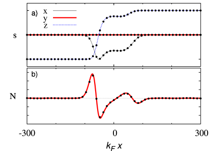
Figure 1: Equilibrium (zero-current) results: (a) Cartesian components of an arbitrarily chosen magnetization ${\bf M}(x)$ (lines); Cartesian components of the calculated spin density ${\bf s}_{\rm eq}(x)$ (solid dots); (b) Exchange torque (solid line) and calculated spin-transfer torque (solid dots).

II.2 Semi-classical

A semi-classical approach to calculating the spin current density is useful for building physical intuition. Accordingly, we write an equation of motion for the spin density of every electron that contributes to the current. This idea has been used in the past, both semi-quantitativelyBerger:1978 and qualitatively.Waintal:2004 Our derivation is based on the behavior of an electron with energy $E$ that moves along the $x$-axis through a uniform magnetic field ${\bf B}_{\rm ex}=B_{\rm ex}\hat{\bf z}$. The wave function for such an electron is

$$\varphi(x,E)=\left(\begin{array}[c]{c}a~{}e^{ik_{+}x}\\ b~{}e^{ik_{-}x}\end{array}\right),$$ (14)

where

$$k_{\pm}^{2}=2mE/\hbar^{2}\pm k_{B}^{2}.$$ (15)

We compute the spin density ${\bf s}(x,E)$ and the spin current density ${\bf Q}(x,E)$ for this electron using the right sides of Eq. (12) and Eq. (13), respectively, with $\psi_{\pm}\to\varphi$.

It is straightforward to check that the components of these densities transverse to the magnetic field satisfy the semi-classical relations

$$Q_{x}=s_{x}\langle v\rangle~{}~{}~{}~{}~{}~{}~{}~{}~{}~{}{\rm and}~{}~{}~{}~{}~{}~{}~{}~{}~{}~{}Q_{y}=s_{y}\langle v\rangle,$$ (16)

where $\langle v\rangle$ is the velocity

$$\langle v\rangle={\hbar\over m}{k_{+}+k_{-}\over 2}={\hbar\over m}\langle k\rangle.$$ (17)

Moreover, the transverse components of the spin density satisfy

$$\langle v\rangle{ds_{x}\over dx} = -{\hbar k_{B}^{2}\over m}s_{y},$$

$$\langle v\rangle{ds_{y}\over dx} = -{\hbar k_{B}^{2}\over m}s_{x}.$$ (18)

These equations are the components of the vector equation

$${d{\bf s}\over dx}=-{k_{B}^{2}\over\langle k\rangle}{\bf s}\times\hat{\bf B}_{\rm ex}$$ (19)

where $\hat{\bf B}_{\rm ex}=\hat{\bf z}$.

We now make the ansatz that all three Cartesian components of the semi-classical majority and minority spin densities ${\bf s}_{\pm}(x,k_{x})$ satisfy Eq. (19) when the direction of the magnetic field varies in space. Specifically, if ${\bf B}_{\rm ex}(x)=B_{\rm ex}\hat{\bf B}_{\rm ex}(x)$, we suppose that

$${d{\bf s}_{\pm}(x,k_{x})\over dx}=-{k_{B}^{2}\over\langle k\rangle}{\bf s}_{\pm}(x,k_{x})\times\hat{\bf B}_{\rm ex}(x),$$ (20)

where $k_{+}$ and $k_{-}$ for ${\bf s}_{+}(x,k_{x})$ are defined by Eq. (15) with $E=\hbar^{2}(k_{x}^{2}-k^{2}_{\rm B})/2m$.KMEvan Similarly, $k_{+}$ and $k_{-}$ for ${\bf s}_{-}(x,k_{x})$ are defined by Eq. (15) with $E=\hbar^{2}(k_{x}^{2}+k^{2}_{\rm B})/2m$. With suitable boundary conditions, we solve the differential equation Eq. (20) to determine the semi-classical, one-electron spin densities. The total, spin-resolved, spin densities follow by inserting these one-electron quantities into

$${\bf s}_{\pm}(x)=\int\left[f_{\pm}({\bf k}-{eE\tau\over\hbar}\bm{\hat{x}})-f_{\pm}({\bf k})\right]{\bf s}_{\pm}(x,k_{x}){k_{x}\over\langle k\rangle}d^{3}{\bf k}.$$ (21)

This equation differs from Eq. (II) by the weighting factor $k_{x}/\langle k\rangle$.ksign This factor guarantees that the flux carried by each electron is proportional to its velocity (see Appendix I). This is confirmed by Fig. 2(b) which shows quantitative agreement between a fully quantum calculation of ${\bf s}(x)$ using Eq. (10), Eq. (12) and Eq. (II) and a semi-classical calculation using Eq. (20) and Eq. (21).

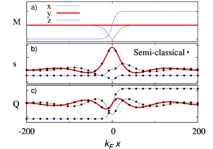
Figure 2: (a) Cartesian components of an imposed magnetization ${\bf M}(x)$ used in the other panels; (b) comparison of quantum (lines) to semi-classical (solid dots) calculations for the Cartesian components of the spin density ${\bf s}(x)$; (c) same comparison for the Cartesian components of the spin current density ${\bf Q}(x)$.

In light of the foregoing, it is reasonable to calculate the semi-classical single-electron spin current density from

$${\bf Q}_{\pm}(x,k_{x})={\bf s}_{\pm}(x,k_{x}){\hbar k_{x}\over m}$$ (22)

and use the second equation in Eq. (II) to find ${\bf Q}_{\pm}(x)$. The correctness of this prescription is illustrated in Fig. 2(c).

III Spin Spiral

As a preliminary to our discussion of domain walls, it is instructive to discuss the spin density and spin current density for a spin spiral—an infinite magnetic structure where the direction of the magnetization rotates continuously as one moves along a fixed axis in space. Spin spirals occur in the ground state of some rare earth metalsJensen:1991 and also for the $\gamma$ phase of iron.Hafner:2002 Here, we focus on a spiral with uniform pitch $p$ where the magnetization rotates in the $x$-$z$ plane, i.e., in Eq. (2),

$$\theta(x)=p\hskip 1.00006ptx~{}~{}~{}~{}~{}~{}~{}~{}~{}~{}{\rm and}~{}~{}~{}~{}~{}~{}~{}~{}~{}~{}\phi(x)=0.$$ (23)

A cartoon version of this ${\bf M}(x)$ is shown in Fig. 3. This figure also defines a local coordinate system that will be useful in what follows. The system $(x^{\prime},y^{\prime},z^{\prime})$ rotates as a function of $x$ so the magnetization ${\bf M}(x)$ always points along $+z^{\prime}$.

CalvoCalvo:1978 solved Eq. (10) to find the eigenstates and eigen-energies of this spin spiral. In our notation,

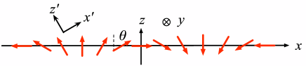
Figure 3: Cartoon of a spin spiral where the magnetization (arrows) rotates uniformly in the $x$-$z$ plane of a fixed coordinate system where $\hat{\bf M}(x)\cdot\hat{\bf z}=\cos\theta$. The inset shows a local coordinate system where ${\bf M}(x)$ always points along the $z^{\prime}$ axis.

$$\varepsilon_{\pm}({\bf k})={\hbar^{2}\over 2m}\left(k^{2}+{1\over 4}p^{2}\pm\sqrt{(k_{x}p)^{2}+k_{B}^{4}}\right),$$ (24)

and

$$\psi_{\pm}({\bf k,r})=e^{i{\bf k\cdot r}}e^{-i\sigma_{y}\theta/2}e^{-i\sigma_{x}\alpha/2}\eta_{\pm},$$ (25)

where

$$\sin\alpha={k_{x}p\over\sqrt{(k_{x}p)^{2}+k_{B}^{4}}},$$ (26)

and

$$\eta_{+}=\left(\begin{array}[c]{c}1\\ 0\end{array}\right),\hskip 20.0pt\eta_{-}=\left(\begin{array}[c]{c}0\\ 1\end{array}\right).\vspace{0.5em}$$ (27)

From these results, it is easy to compute the single-electron spin densities defined in Eq. (12). In the local $(x^{\prime},y^{\prime},z^{\prime})$ frame,

$${\bf s^{\prime}}_{\pm}(x,k_{x})=\pm(0,\sin\alpha,\cos\alpha).$$ (28)

The corresponding calculation of the single-electron spin current densities Eq. (22) is straightforward but tedious and not very illuminating. Therefore, we pass directly to the total spin current density calculated by summing over all electrons as indicated in the second line of Eq. (II). Again in the local $(x^{\prime},y^{\prime},z^{\prime})$ frame,

$${\bf Q^{\prime}}(x)=A(p,k_{\rm B})(0,0,1).$$ (29)

where $A(p,k_{\rm B})$ is a constant. This shows that ${\bf Q}(x)\propto{\bf M}(x)$, i.e., the spin current density for a free electron spin spiral is perfectly adiabatic. Wessely et al.Nordstrom:2005 found consistent results in their density functional calculation of the steady-state spin current density associated with the helical spin density wave in erbium metal. We emphasize that Eq. (29) is independent of pitch for an infinite spin spiral. As we discuss below, a similar independence does not hold for domain walls. In that case, wide walls are adiabatic, but narrow ones are not.

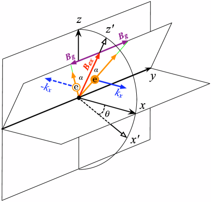
Figure 4: Electrons (wave vector $k_{x}$) and holes (wave vector $-k_{x}$) move in an effective field that is the sum of the exchange field ${\bf B}_{\rm ex}(x)\parallel\hat{\bf z}^{\prime}$ and a fictitious, velocity-dependent “gradient” field induced by the spatial dependence of the exchange field. The spins align to the total effective field in an infinite spin spiral. The $x$ axis lies in $x^{\prime}$-$z^{\prime}$ plane.

The semi-classical formula Eq. (22) provides an appealing way to understand the adiabaticity of the spin current density in the spin spiral defined by Eq. (23). The key point is that the angle $\alpha$ in Eq. (26) which fixes the direction of ${\bf s}_{\pm}(x,k_{x})$ in Eq. (28) is positive when $k_{x}$ is positive and negative when $k_{x}$ is negative (Fig. 4). Moreover, for every $k_{x}$ electron that contributes to the shifted Fermi surface sums in Eq. (II), there is a contribution from a $-k_{x}$ hole. Now, a hole has opposite spin density to an electron and the spin current density Eq. (22) contains an additional factor of $k_{x}$. Therefore, the two spin density vectors in Fig. 4 subtract to give a net spin density along $\hat{\bf y}$ while the corresponding two spin current density vectors add to give a net spin current density along $\hat{\bf z}^{\prime}$. This occurs for all $k_{x}$ in the sums so ${\bf Q}(x)$ aligns exactly with the local exchange field and thus with the local magnetization.

The opposite situation occurs for fully occupied states below the Fermi energy. The spins of the forward and backward moving electrons combine to produce a net moment aligned with the exchange field, as necessary for self-consistency. Further, the spin currents, with the additional factor of $k_{x}$ add to give a net spin current along $\hat{\bf y}$, so that its gradient gives the correct form of the phenomenological exchange torque density.

To summarize: an electric current that passes through a spin spiral generates a spin accumulation with a component transverse to the magnetization. The spin current density possesses no such component due to pairwise cancellation between forward and backward moving spins of the same type (majority or minority). Moreover, since the cancellation occurs within each band, the final result is insensitive to the details of intraband scattering.

It remains only to understand the origin of the misalignment angle $\alpha$. Why does each spin not simply align itself with ${\bf B}_{\rm ex}$? BergerBerger:1978 was the first to notice this fact and the physics was made particularly clear by Aharonov and Stern.Aharonov:1992 These authors studied the adiabatic approximation for a classical magnetic moment that moves in a slowly varying field ${\bf B}(x)$. Not obviously, the moment behaves as if were subjected to a effective magnetic field ${\bf B}_{\rm eff}(x)$ that is the sum of ${\bf B}_{\rm ex}(x)$ and a fictitious, velocity-dependent, “gradient” field ${\bf B}_{\rm g}(x)$ that points in the direction $\nabla\hat{\bf B}(x)\times\hat{\bf B}(x)$. For our problem,

$${\bf B}_{\rm eff}={\bf B}_{\rm ex}+{\hbar^{2}k_{x}\over 2m\mu}{d\hat{\bf B}_{\rm ex}\over dx}\times\hat{\bf B}_{\rm ex}.$$ (30)

The presence of this gradient field is apparent from Eq. (24) where the square root is proportional to $|{\bf B}_{\rm eff}|$. The adiabatic solution corresponds to perfect alignment of the moment with ${\bf B}_{\rm eff}(x)$. This alignment is indicated in Eq. (28) and in Fig. 4. More generally, the expected motion of the magnetic moment is precession around ${\bf B}_{\rm eff}(x)$.Nevertheless, as indicated above, the total spin current density for the spin spiral aligns with ${\bf B}_{\rm ex}(x)$ (which is the conventional definition of adiabaticity for this quantity) when the net effect of all conduction electrons is taken into account.

IV Domain Walls

Our main interest is the spin-transfer torque associated with domain walls that connect two regions of uniform and antiparallel magnetization. A realistic wall of this kind can be described by Eq. (2) withHubert:1998

$$\theta(x)=\pi/2-\arcsin\left[\tanh\left(x/w\right)\right],$$ (31)

The wall is Néel-type if $\phi(x)=0$ and Bloch-type if $\phi(x)=\pi/2$. We will speak of the domain wall width $w$ as “long” or “short” depending on whether $w$ is large or small compared to the characteristic length

$$L={E_{F}\over E_{\rm ex}}{1\over k_{F}}={k_{F}\over k_{B}^{2}}.$$ (32)

Intuitively, the adiabatic approximation should be valid when $w\gg L$. When applied to Eq. (II), the predicted adiabatic spin-transfer torque for our model is

$${\bf N}_{\rm ad}(x)=-{\hbar\over 2}\eta{neE\tau\over m}\partial_{x}\hat{\bf M}(x),$$ (33)

where $n$ is the electron density, and $\eta$ is the polarization of the current. The calculations required to check this for long domain walls are difficult quantum mechanically (for numerical reasons) but straightforward semi-classically. At the single-electron level, adiabaticity again corresponds to alignment of the spin moment with the effective field defined in Eq. (30). The results for a typical long wall (Fig. 5) demonstrate that summation over all electrons produces alignment of ${\bf Q}(x)$ with ${\bf M}(x)$ so the adiabatic formula Eq. (33) is indeed correct in this limit.

For short walls, we have carried out calculations of ${\bf N}_{\rm st}(x)$ both quantum mechanically and semi-classically. The two methods agree very well with one another (see Fig. 2) but not with the proposed form Eq. (1). Bearing in mind that, when the magnetization changes, $\hat{\bf x}^{\prime}$ points along $\partial_{x}{\bf M}$ and $\hat{\bf y}$ points along ${\bf M}\times\partial_{x}{\bf M}$, our result for the spin-transfer torque is

$${\bf N}_{\rm st}(x)={\bf N}_{\rm ad}(x)+a(x)\hat{\bf x}^{\prime}+b(x)\hat{\bf y}.$$ (34)

Figure 5: Distributed spin-transfer torque for a long Nèel domain wall with $w=50$ and $L=6.25$ ($k_{F}=1$ and $k_{B}=0.4$): semi-classical calculation of ${\bf N}_{\rm st}$ (solid dots) compared to Eq. (33) for ${\bf N}_{\rm ad}(x)$ (solid curve).

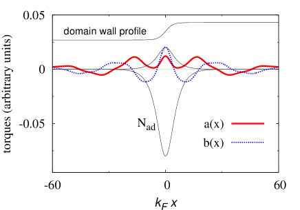
Figure 6: Distributed spin-transfer torque for a short Nèel domain wall with $w=4$ and $L=6.25$ ($k_{F}=1$ and $k_{B}=0.4$): in-plane piece $a(x)$ (heavy solid curve); out-of-plane piece $b(x)$ (dashed curve); adiabatic prediction (light solid curve); second term in Eq. (1) scaled to match the maximum of $b(x)$ (light solid curve).

${\bf N}_{\rm st}(x)$ differs from ${\bf N}_{\rm ad}(x)$ because gradients in the gradient field induce single electron spin moments to precess around ${\bf B}_{\rm eff}(x)$ rather to align perfectly with it. Fig. 6 shows $a(x)$ and $b(x)$ as calculated for a typical short domain wall. The associated torques lie in the plane of the magnetization and perpendicular to that plane, respectively. These non-adiabatic contributions to the torque are both oscillatory functions of position that do not go immediately to zero when the the magnetization becomes uniform. In other words, $a(x)$ and $b(x)$ are generically non-local functions of the magnetization ${\bf M}(x)$. The positive-valued function that falls to zero at the edges of the domain wall (light solid curve in Fig. 6) is the second function in Eq. (1) with $c_{2}$ chosen to match $b(x)$ at their common maximum. Evidently, the proposed torque function Eq. (1) gives at best a qualitative account of the out-of-plane non-adiabatic torque.

A convenient measure of the degree of non-adiabaticity of the spin-transfer torque is

$${\cal Q}={{\rm max}\,|\,b(x)\,|\over{\rm max}\,|\,N_{\rm ad}(x)\,|}.$$ (35)

Figure 7: Non-adiabaticity in Eq. 35 versus wall width scaled by the characteristic length in Eq. (32). Note the logarithmic scale.

Fig. 7 plots this quantity as a function of scaled domain wall width $w/L$ on a log scale. The observed exponential decrease of the non-adiabatic torque as the wall width increases can be understood from the work of Dugaev et al.Dugaev:2002 These authors treat the gradient field in Eq. (30) as a perturbation and calculate the probability for an electron in a $(k_{x}\uparrow)$ state to scatter into a $(k^{\prime}_{x}\downarrow)$ state in the Born approximation. If we choose $k_{x}$ and $k^{\prime}_{x}$ as $k_{F}^{+}$ and $k_{F}^{-}$, respectively, their results imply that the probability ${\cal P}$ that a majority electron retains its spin and becomes a minority electron as it passes through a domain wall is

$${\cal P}\propto\exp(-\gamma w/L),$$ (36)

where $\gamma$ is a constant of order unity. This rationalizes the result plotted in Fig. 7 because the magnitude of the minority spin component determines the amplitude of the spin precession around ${\bf B}_{\rm eff}(x)$ and thus the magnitude of the non-adiabatic component of ${\bf s}$ and ${\bf Q}$ in Eq. (22). In fact, $N_{\rm ad}\propto 1/w$, so it is the case that

$${\rm max}\,|\,b(x)\,|\propto{1\over w}\exp(-\gamma w/L).$$ (37)

The slope of the straight line in Fig. 7, i.e., the value of the constant $\gamma$ in Eq. (36) depends on the sharpness of the domain wall. Using Eq. (31) and other simple domain wall profile functions, it is not difficult to convince oneself that a suitable measure of domain wall sharpness is the maximum value of the second derivative $\theta^{\prime\prime}(x)$ for walls with the same width. The numerical results shown in Fig. 8 confirm this to be true. The sharper the domain wall, the less rapidly the non-adiabatic torque disappears with increasing domain wall width.

Figure 8: Dependence of $\gamma$ in Eq. (36) on domain wall sharpness: Squares are calculated points. Straight line is a guide to the eye that passes through the origin.

V Relation to Other Work

V.0.1 Waintal & Viret

Waintal and ViretWaintal:2004 (WV) used a free-electron Stoner model and the Landauer-Büttiker formalism to calculate the spin transfer torque associated with a Néel wall with magnetization Eq. (2) and

$$\quad\theta(x) = \left\{\begin{array}[]{lr}0,&x<-w\\ \displaystyle(\pi/2)\left(x/w+1\right),&-w\leq x\leq w\\ \pi,&x>w.\end{array}\right.$$ (41)

For this wall profile (which is exactly one half-turn of a uniform spin spiral in the interval $-w\leq x\leq w$), WV reported oscillatory non-adiabatic contributions to the torque similar to our functions $a(x)$ and $b(x)$. This contrasts with the perfect adiabaticity we found in Sec. III for the infinite spin spiral. Moreover, the amplitude of the non-adiabatic torque reported by WV for this wall decreases only as $1/w$ rather than $(1/w)\exp(-\gamma w/L)$ as we found above.

The disparities between Ref. Waintal:2004, and the present work all arise from the unphysical nature of the domain wall Eq. (41). Specifically, the divergence of $\theta^{\prime\prime}(x)$ at $x=\pm w$ locates this wall at the origin of Fig. 8 where $\gamma=0$. This brings their result into agreement with Eq. (37). Any rounding of the discontinuity in slope at $x=\pm w$ would yield a finite value for $\theta^{\prime\prime}(x)$ and thus a non-zero value of $\gamma$.

In Appendix II, we calculate the spin-transfer torque for the wall Eq. (41) using our methods. Qualitatively, the pure $1/w$ behavior of the non-adiabatic torque comes from the fact that there is a sudden jump in $\theta^{\prime}(x)$ at $x=\pm w$. There is a corresponding jump in the direction of ${\bf B}_{\rm eff}(x)$ as defined by Eq. (30). Spins propagating along the the $x$-axis cannot follow this abrupt jump and thus precess around the post-jump field direction with an amplitude determined by the sine of the angle between the before-and-after field directions. The latter is proportional to the jump in $\theta^{\prime}(x)$, which is $\pi/2w$ for the wall Eq. (41).

V.0.2 Zhang & Li

In spin spirals and long domain walls, we find that the non-equilibrium spin current is adiabatic, i.e., ${\bf Q}(x)$ is aligned with ${\bf M}(x)$ [or ${\bf B}_{\rm ex}(x)$]. At the same time, we find in both cases that the non-equilibrium spin density ${\bf s}(x)$ is not aligned with the magnetization; there is component of ${\bf s}(x)$ transverse to ${\bf M}(x)$. The corresponding transverse component of the spin current density cancels between pairs of electrons moving in opposite directions. Zhang and LiZhang:2004 found exactly the same form of non-equilibrium spin accumulation (called $\delta{\bf m}(x)$ by them) using a phenomenological theory. They proposed that this non-equilibrium spin density relaxes by spin-flip scattering toward alignment with the magnetization. Such a relaxation would produce a non-adiabatic torque of the form given by the second term in Eq. (1). The correctness of this predicted non-adiabatic torque depends on the correctness of the assumed model for relaxation of transverse spin accumulation through spin flip scattering.

Zhang and Li assume a form for the rate of spin flip scattering, $\delta{\bf m}/\tau_{\rm sf}$, that has been used successfully as a phenomenological description of longitudinal spin relaxation in systems with collinear magnetization. While it is plausible to extend this form, as they do, to describe transverse spin relaxation in non-collinear systems, our calculations indicate that it is not likely to be correct. Our reasoning is simplest to appreciate for a spin spiral with small pitch $p$. In this limit, Eqs. (26) and (28) show that the transverse component of the spin for every electron eigenstate is proportional to its velocity. This means that the majority band electrons contribute a transverse spin accumulation and an electric current that are proportional to one other. The same is true, separately, for the minority band electrons. This conclusion is independent of the details of the electron distribution. Therefore, for a fixed total current, it is impossible to relax the transverse spin accumulation without changing the longitudinal polarization of the current. No such change occurs in the model in Ref. Zhang:2004, , casting doubt on the validity of the form of the spin flip scattering assumed there.

Microscopic considerations also argue against this form of the relaxation. As we have emphasized, the natural basis for an electron spin moving though a non-collinear magnetization is not along the local exchange field ${\bf B}_{\rm ex}(x)$, but rather along a local effective field ${\bf B}_{\rm eff}(x)$, which includes the corrections due to the gradient of the magnetization [see Eq. (30)]. Any spin that deviates from parallel or antiparallel alignment with the effective field will precess around the effective field, and on average will point parallel or antiparallel. Thus, we expect that there is no tendency for electron spins moving in a non-uniform magnetization to align themselves with the local exchange field ${\bf B}_{\rm ex}(x)$ by spin-flip scattering (or any other mechanism). Rather, the adiabatic solution is precisely alignment of their spins with the local effective field ${\bf B}_{\rm eff}(x)$. Without further microscopic justification, we believe that the phenomenological form of spin flip scattering assumed in Ref. Zhang:2004, should not be used in systems with non-collinear magnetizations. Hence, this analysis argues against the existence of the resulting contribution to the “non-adiabatic” torque from spin flip scattering.

VI Scattering

We do not explicitly treat scattering in any of our calculations. However, the distribution function in Eq. (II), a shifted Fermi distribution, is an approximate solution of the Boltzmann equation in certain limits. First, the electric field must be small enough that the transport is in the linear regime. Then, the appropriate limits are determined by three important length scales, the Fermi wavelength, the mean free path, and the characteristic length of the structure, either the pitch of the spin spiral or the width of the domain wall. In all cases, we consider the limit in which the Fermi wavelength is short compared to the mean free path. This limit allows the description of the states of the system in terms of the eigenstates of the system in the absence of scattering. Different limits apply to the cases of domain walls and of spin spirals because the distribution functions are interpreted differently for these two structures.

We use the Boltzmann equation in two different ways. When the mean free path is much longer than the characteristic size of the structure, the distribution function describes the occupancy of the eigenstates of the entire system. This distribution function is independent of the spatial coordinate and we refer to this approach as global. In the opposite limit, the distribution function is spatially varying and describes the occupancy of eigenstates of the local Hamiltonian, which includes the exchange field and the gradient field. We refer to this approach as local, as the distribution function can vary spatially.

For spin spirals, the distribution functions are shifted Fermi functions of the eigen-energies of the spin spiral. In the limit that the pitch of the spiral is much shorter than the mean free path, the shifted distribution given in Eq. (II) is a solution of the global Boltzmann equation in the relaxation time approximation. The distribution function also becomes a solution in the opposite limit, where the mean free path is much shorter than the pitch of the spiral. In this limit, the Boltzmann equation is considered locally rather than globally. At each point in space the states are subject to the local exchange field, and the local gradient field. The distribution function is defined for states that are locally eigenstates of the sum of the fields. The local distribution function is given by the adiabatic evolution in the rotating reference frames of the distribution function specified in Eq. (II). In the limit that the pitch of the spiral goes to infinity, this distribution function locally solves the Boltzmann equation in the relaxation time approximation. Thus, for spin spirals, the distribution function given in Eq. (II) is a solution in the limits that the mean free path is much greater than or much less than the pitch. We speculate that the corrections in between these limits are small.

Domain walls are not uniform in the way that spin spirals are, so the distribution functions need to be given a different interpretation. For these structures, the distribution function is determined from the properties of the states in the leads. For example, in the Landauer-Büttiker approach to this problem,Waintal:2004 scattering is ignored in the domain wall itself and confined to the “leads” adjacent to it (these leads are assumed to be “wide” and function as electron reservoirs). An applied voltage is assumed to raise the energy of electron states in one lead relative to the other. Thus, in a formula like Eq. (II), the distribution function is shifted in energy rather than in velocity.

We also do not treat scattering within the domain wall explicitly, but we assume that the wall is bounded by long leads that are as “narrow” as the domain wall region and have resistances per unit length that are comparable to that of the domain wall region. Thus, the distribution of the states approaching the domain wall region is similar to the distribution of states in an extended wire, i.e., to that given by Eq. (II). For domain walls in long wires, the distribution function for left going states is determined by the right lead and for right going states by the left lead. With this interpretation, the distribution given in Eq. (II) is a solution in the limit that the scattering in the domain wall is weak, that is, the domain wall is much narrower than the mean free path.

The distribution in Eq. (II) is also a solution in the limit that the mean free path is much shorter than the domain wall width. Since the Fermi wave length is much shorter than the mean free path, it is much less than the domain wall width. In this case, quantum mechanical reflection is negligible and the quantum mechanical states are closely related to the semiclassical trajectories. With a similar interpretation of the distribution function as was made for the spin spirals in this limit, the same conclusion holds for the domain walls.

VII Summary & Conclusion

In this paper, we analyzed spin-transfer torque in systems with continuously variable magnetization using previous results of CalvoCalvo:1978 for the eigenstates of an infinite spin spiral and of Aharonov and SternAharonov:1992 for the classical motion of a magnetic moment in an inhomogeneous magnetic field. Adiabatic motion of individual spins corresponds to alignment of the spin moment not with the exchange field (magnetization) but with an effective field that is slightly tilted away form the exchange field by an amount that depends on the spatial gradient of the magnetization. Nevertheless, when summed over all conduction electrons, the spin current density is parallel to the magnetization both for an infinite spin spiral and for domain walls that are long compared to a characteristic length $L$ that depends on the exchange energy and the Fermi energy.

Non-adiabatic corrections to the spin-transfer torque occur only for domain walls with widths $w$ that are comparable to or smaller than $L$. The non-adiabatic torque is oscillatory and non-local in space with an amplitude that decreases as $w^{-1}\exp(-\gamma w/L)$. The constant $\gamma$ is largest for walls with the sharpest magnetization gradients. This suggests that non-adiabatic torques may be important for spin textures like vortices where the magnetization varies extremely rapidly.

Using microscopic considerations, we have also argued that the role of the gradient field to tilt spins away from the exchange field casts serious doubt on a recent proposal by Zhang and LiZhang:2004 that a non-negligible non-adiabatic contribution to the torque arises from relaxation of the non-equilibrium spin accumulation to the magnetization vector by spin flip scattering. We conclude that, if the second term in Eq. (1) truly accounts for the systematics of current-driven domain wall motion, the physics that generates this term still remains to be identified.

Finally, we have carefully discussed the role of scattering in this problem with particular emphasis on the approximation used here to neglect scattering within the domain wall itself but to treat the adjacent ferromagnetic matter as bulk-like. We argue that this approximation is valid in limits that either include or bracket the most interesting experimental situations and therefore is likely to be generally useful.

VIII Acknowledgment

One of us (J.X.) is grateful for support from the Department of Energy under grant DE-FG02-04ER46170.

Appendix I: Semi-Classical Weighting Factor

The weighting factor $k_{x}/\langle k\rangle$ used in Eq. (21) brings the amplitude of the dynamic (transverse) part of the semi-classical, one-electron spin density into accord with the corresponding quantum mechanical amplitude. This can be seen from a simple model problem that we solve both quantum mechanically and semi-classically. Namely, a spin initially oriented along the $+\hat{\bf x}$ direction propagates from $x=-\infty$ to $x=\infty$ through a magnetization that changes abruptly from ${\mathbf{M}}(x)=M(1,0,0)$ for $x<0$ to ${\mathbf{M}}(x)=M(0,0,1)$ for $x\geq 0$. For $x<0$, the eigenstates are

$$\psi_{\uparrow}^{-}(x)={1\over\sqrt{2}}\left(\begin{array}[c]{c}1\\ 1\end{array}\right)e^{ik_{\uparrow}x},\quad\psi_{\downarrow}^{-}(x)={1\over\sqrt{2}}\left(\begin{array}[c]{c}1\\ -1\end{array}\right)e^{ik_{\downarrow}x},$$ (43)

and for $x>0$, the eigenstates are

$$\psi_{\uparrow}^{+}(x)=\left(\begin{array}[c]{c}1\\ 0\end{array}\right)e^{ik_{\uparrow}x},\quad\psi_{\downarrow}^{+}(x)=\left(\begin{array}[c]{c}0\\ 1\end{array}\right)e^{ik_{\downarrow}x}.$$ (44)

If we choose the incoming state as

$$\psi(x)=\psi_{\uparrow}^{-}(x),$$ (45)

the reflection and transmission amplitudes for spin flip $(r_{\uparrow\downarrow},t_{\uparrow\downarrow})$ and no spin flip $(r_{\uparrow\uparrow},t_{\uparrow\uparrow})$ are determined by matching the total wave function and its derivative at $x=0$:

$$\psi_{\uparrow}^{-}+r_{\uparrow\uparrow}(\psi_{\uparrow}^{-})^{*}+r_{\uparrow\downarrow}(\psi_{\downarrow}^{-})^{*} = t_{\uparrow\uparrow}\psi_{\uparrow}^{+}+t_{\uparrow\downarrow}\psi_{\downarrow}^{+}$$

$$k_{\uparrow}\psi_{\uparrow}^{-}-r_{\uparrow\uparrow}k_{\uparrow}(\psi_{\uparrow}^{-})^{*}-r_{\uparrow\downarrow}k_{\downarrow}(\psi_{\downarrow}^{-})^{*} = t_{\uparrow\uparrow}k_{\uparrow}\psi_{\uparrow}^{+}+t_{\uparrow\downarrow}k_{\downarrow}\psi_{\downarrow}^{+}.$$

It is straightforward to confirm that these equations are solved by

$$r_{\uparrow\uparrow}={k_{\uparrow}^{2}-k_{\downarrow}^{2}\over k_{\uparrow}^{2}+6k_{\uparrow}k_{\downarrow}+k_{\downarrow}^{2}} r_{\uparrow\downarrow}={2k_{\uparrow}(k_{\downarrow}-k_{\uparrow})\over k_{\uparrow}^{2}+6k_{\uparrow}k_{\downarrow}+k_{\downarrow}^{2}}$$ ,

$$t_{\uparrow\uparrow}={4\sqrt{2}k_{\uparrow}k_{\downarrow}\over k_{\uparrow}^{2}+6k_{\uparrow}k_{\downarrow}+k_{\downarrow}^{2}} t_{\uparrow\downarrow}={2\sqrt{2}k_{\uparrow}(k_{\uparrow}+k_{\downarrow})\over k_{\uparrow}^{2}+6k_{\uparrow}k_{\downarrow}+k_{\downarrow}^{2}}.$$ ,

We are interested in the transmitted wave function,

$$\psi_{\rm tr}(x)=t_{\uparrow\uparrow}\psi_{\uparrow}^{+}(x)+t_{\uparrow\downarrow}\psi_{\downarrow}^{+}(x)=\left(\begin{array}[c]{c}t_{\uparrow\uparrow}e^{ik_{\uparrow}x}\\ t_{\uparrow\downarrow}e^{ik_{\downarrow}x}\end{array}\right),$$ (49)

which carries a spin density,

$${\mathbf{s}}_{\rm tr}^{\rm qm}(x)={\hbar\over 2}\left[2t_{\uparrow\uparrow}t_{\uparrow\downarrow}\cos(\delta kx),2t_{\uparrow\uparrow}t_{\uparrow\downarrow}\sin(\delta kx),(t_{\uparrow\uparrow}^{2}-t_{\uparrow\downarrow}^{2})\right],$$ (50)

where $\delta k=k_{\uparrow}-k_{\downarrow}$. Notice that the oscillation is transverse to the $x\to\infty$ magnetization and of amplitude $\hbar t_{\uparrow\uparrow}t_{\uparrow\downarrow}$.

If we analyze the same problem semi-classically, a majority electron propagates freely until it reaches $x=0$. At that point, the electron feels a magnetization perpendicular to its magnetic moment and begins precession around that magnetization with unit amplitude. The associated spin density is

$${\mathbf{s}}_{\rm tr}^{\rm sc}(x)={\hbar\over 2}\left[\cos(\delta kx),\sin(\delta kx),0\right].$$ (51)

Comparing Eq. (50) to Eq. (51) shows that the transverse oscillation amplitudes will be equal if we multiply the semi-classical result by the weighting factor

$$2t_{\uparrow\uparrow}t_{\uparrow\downarrow}={32k_{\uparrow}^{2}k_{\downarrow}(k_{\uparrow}+k_{\downarrow})\over(k_{\uparrow}^{2}+6k_{\uparrow}k_{\downarrow}+k_{\downarrow}^{2})^{2}}\approx{2k_{\uparrow}\over k_{\uparrow}+k_{\downarrow}}={k_{x}\over\langle k\rangle}.$$ (52)

Fig. 9 illustrates the quality of the approximation in Eq. (52) if we identify $k_{\uparrow}$ and $k_{\downarrow}$ with $k^{+}_{F}$ and $k^{-}_{F}$ (respectively) in Eq. (5). Of course, $k_{x}$ plays the role of $k_{\uparrow}$ in Eq. (21).

Figure 9: The semi-classical weighting factor for the spin density. Solid (dotted) curve is the expression on the left (right) side of the $\approx$ symbol in Eq. (52).

Appendix II: Spin Spiral Domain Wall

The semi-classical spin density associated with electron propagation through a magnetization like Eq. (2) is the solution of Eq. (20) with suitable boundary conditions. Choosing $\phi=0$, we simplify the notation by using the prefactor $\lambda=k_{B}^{2}/\langle k\rangle$ and an overdot for $d/dx$ to write the components of Eq. (20) as

$$\dot{s}_{x} = -\lambda s_{y}\cos\theta$$ (53)

$$\dot{s}_{y} = -\lambda s_{z}\sin\theta+\lambda s_{x}\cos\theta$$ (54)

$$\dot{s}_{z} = \lambda s_{y}\sin\theta.$$ (55)

In the local frame $(x^{\prime},y^{\prime},z^{\prime})$ defined in Fig. 3, the components of the spin density,

$$s^{\prime}_{x} = s_{x}\cos\theta-s_{z}\sin\theta$$ (56)

$$s^{\prime}_{y} = s_{y}$$ (57)

$$s^{\prime}_{z} = s_{x}\sin\theta+s_{z}\cos\theta,$$ (58)

satisfy

$$\dot{s}^{\prime}_{x} = -\lambda s^{\prime}_{y}-s^{\prime}_{z}\dot{\theta}$$ (59)

$$\dot{s}^{\prime}_{y} = \lambda s^{\prime}_{x}$$ (60)

$$\dot{s}^{\prime}_{z} = s^{\prime}_{x}\dot{\theta}.$$ (61)

Eliminating $s^{\prime}_{y}$ gives

$$\ddot{s}^{\prime}_{x}+(\lambda^{2}+\dot{\theta}^{2})s^{\prime}_{x}+s^{\prime}_{z}\ddot{\theta}=0.$$ (62)

The differential Eq. (62) cannot be solved analytically for realistic domain wall profiles. However, it is easily solvable for the wall defined by Eq. (41) where one-half turn of a spin spiral with pitch $p=\pi/2w$ connects two regions with uniform (but reversed) magnetization. In the limit $\pi/w\ll\lambda$ of a long wall, the components of the spin density transverse to the wall magnetization for the range $x\in[-w,w]$ are (after multiplying the weighting factor $k_{x}/\langle k\rangle$ for the semi-classical approach)

$$s^{\prime}_{x}(x) = {\hbar\over 2}{k_{x}\over\langle k\rangle}{\pi\over 2w\lambda}\sin(\lambda(x\pm w))$$

$$s^{\prime}_{y}(x) = {\hbar\over 2}{k_{x}\over\langle k\rangle}{\pi\over 2w\lambda}\left[1-\cos(\lambda(x\pm w))\right],$$ (63)

where the plus (minus) refers to electrons that flow from left (right) to right (left). The associated spin current density and spin transfer torque carried by each electron follow from Eq. (22) and Eq. (7), respectively. Bearing in mind that $\hat{\bf x}^{\prime}$ varies with $x$, our final result for the torque (in the local frame) generated by a single electron moving from right to left is

$$N^{\prime}_{x} = {\hbar\over 2}{\hbar k_{x}\over m}{k_{x}\over\langle k\rangle}{\pi\over 2w}\left[1-\cos\lambda(x-a)\right]~{}\hat{\bf x}^{\prime}$$

$$N^{\prime}_{y} = {\hbar\over 2}{\hbar k_{x}\over m}{k_{x}\over\langle k\rangle}{\pi\over 2w}\sin\lambda(x-a)~{}\hat{\bf y}.$$ (64)

This may be compared with the results of Ref. Waintal:2004, which pertain to the entire ensemble of conduction electrons.

References

- (1) A. Fert, J.-M. George, H. Jaffrès, R. Mattana, and P. Seneor, Europhysics News 34, 227 (2003). Available at www.europhysicsnews.com/full/24/article9/article9.html
- (2) J. C. Slonczewski, J. Magn. Magn. Mater. 159, L1 (1996); L. Berger, Phys. Rev. B 54, 9553 (1996).
- (3) S.I. Kiselev, J.C. Sankey, I.N. Krivorotov, N.C. Emley, R.J. Schoelkopf, R.A. Buhrman, and D.C. Ralph, Nature (London) 425, 380 (2003).
- (4) L. Berger, J. Appl. Phys. 49, 2156 (1978).
- (5) Ya. B. Bazaliy, B.A. Jones, and S.-C. Zhang, Phys. Rev. B 57, R3213 (1998).
- (6) L. Gan, S.H. Chung, K.H. Ashenbach, M. Dreyer, and R.D. Gomez, IEEE Trans. Magn. 36, 3047 (2000); H. Koo, C. Krafft, and R.D. Gomez, Appl. Phys. Lett. 81, 862 (2002); J. Grollier, P. Boulenc, V. Cros, A. Hamzic, A. Vaures, A. Fert, and G. Faini, Appl. Phys. Lett. 83, 509 (2003); M. Kläui, C.A.F Vaz, J.A.C. Bland, W. Wernsdorfer, G. Faini, E. Cambril, and L.J. Heyderman, Appl. Phys. Lett. 83, 105 (2003); M. Tsoi, R.E. Fontana, and S.S. Parkin, Appl. Phys. Lett. 83, 2617 (2003); N. Vernier, D.A. Allwood, D. Atkinson, M.D. Cooke, and R.P. Cowburn, Europhys. Lett. 65, 526 (2004); A. Yamaguchi, T. Ono, S. Nasu, K. Miyake, K. Mibu, and T. Shinjo, Phys. Rev. Lett. 92, 077205 (2004); C. Lim, T. Devolder, C. Chappert, J. Grollier, V. Cros, A. Vaurères, A. Fert, and G. Faini, Appl. Phys. Lett. 84, 2820 (2004); E. Saitoh, H. Miyajima, T. Yamaoka, and G. Tatara, Nature (London) 432 203 (2004); M. Yamanouchi, D. Chiba, F. Matsukura, and H. Ohno, Nature (London) 428, 539 (2004).
- (7) X.Waintal and M. Viret, Europhys. Lett. 65, 427 (2004).
- (8) G. Tatara and H. Kohno, Phys. Rev. Lett. 92, 086601 (2004).
- (9) S. Zhang and Z. Li, Phys. Rev. Lett. 93, 127204 (2004); J. He, Z. Li, and S. Zhang, cond-mat/0508736; Z. Li, J. He, and S. Zhang, cond-mat/0508735.
- (10) A. Thiaville, Y. Nakatani, J. Miltat, and Y. Suzuki, Europhys. Lett. 69, 990 (2005).
- (11) S.E. Barnes and S. Maekawa, Phys. Rev. Lett. 95, 107204 (2005).
- (12) M.D. Stiles, A. Zangwill, Phys. Rev. B 66, 014407 (2002); The transverse spin current in this work decays algebraically rather than exponentially. An estimate of the “dephasing length” is the typical distance over which the transverse spin current decays to 10% of its initial value.
- (13) S. Zhang, P.M. Levy, and A. Fert, Phys. Rev. Lett. 88, 236601 (2002). The transverse spin current in this work decays exponentially with a scale set by a “transverse spin diffusion length”.
- (14) L. Berger, Phys. Rev. B 33 1572 (1986).
- (15) A. Thiaville, Y. Nakatani, J. Miltat, and N. Vernier, J. Appl. Phys. 95, 7049 (2004).
- (16) D. Ravelosona, D. Lacour, J.A. Katine, B.D. Terris, and C. Chapppert, Phys. Rev. Lett. 95, 117203 (2005).
- (17) See M. Kläui, P.-O. Jubert, R. Allenspach, A. Bischof, J.A.C. Bland, G. Faini, U. Rüdiger, C.A.F. Vaz, L. Vila, and C. Vouille, Phys. Rev. Lett. 95, 026601 (2005) and references therein.
- (18) In reality, the magnetization is oppositely directed to the spin density since the g-factor for electrons is negative. For simplicity, we ignore this sign difference and assume that the magnetization is parallel to the spin density. Care is required when using spin currents to compute torques on magnetizations.
- (19) The spin current density is a tensor quantity (Ref. Stiles:2002, ). However, since the current defines the only relevant direction in space for this problem, we supress this dependence and use the components of the vector to denote the Cartesian components of the spin degree of freedom in the spin current density.
- (20) When is sufficiently small, as we assume here, the difference in the square brackets in Eq. (II) is zero except in the immediate vicinity of the Fermi surface. In this limit, the integral over reciprocal space in Eq. (II) reduces to an integral over wave vectors restricted to the Fermi surface, reflecting the fact that non-equilibrium transport involves states near the Fermi surface. The reduction of the integration in this manner leads to the linearized Boltzmann equation. On the other hand, the equilibrium spin densities and currents, as shown in Fig. 1, involve contributions from all occupied states, not just those near the Fermi surface.
- (21) W.F. Brown, Jr. Magnetostatic Principles in Ferromagnetism (North-Holland, Amsterdam, 1962). See equation (7.45); See also Appendix A in M.D. Stiles, J. Xiao, and A. Zangwill, Phys. Rev. B 69, 054408 (2004).
- (22) For , otherwise , which ensures that is continous function of .
- (23) We note that and have the same algebraic sign.
- (24) J. Jensen and A.K. Mackintosh Rare Earth Magnetism (Oxford University Press, Oxford, 1991).
- (25) M. Marsman and J. Hafner, Phys. Rev. B 66, 224409 (2002).
- (26) Miguel Calvo, Phys. Rev. B 18, 5073 (1978).
- (27) O. Wessely, B. Skubic, and L. Nordström, cond-mat/0511224.
- (28) Y. Aharonov and A. Stern, Phys. Rev. Lett. 69, 3593 (1992).
- (29) A. Hubert and R. Schäfer, Magnetic Domains (Springer, Berlin, 1998).
- (30) V. K. Dugaev, J. Barnaś, A. Lusakowski, and L. A. Turski, Phys. Rev. B 65, 224419 (2002). See also G.C. Cabrera and L.M. Falicov, Phys. Stat. Solidi B 61 539 (1974).