Structural transitions and non-monotonic relaxation processes in liquid metals

Abstract

Structural transitions in melts as well as their dynamics are considered. It is supposed that liquid represents the solution of relatively stable solid-like locally favored structures (LFS) in the surrounding of disordered normal-liquid structures. Within the framework of this approach the step changes of liquid Co viscosity are considered as liquid-liquid transitions. It is supposed that this sort of transitions represents the cooperative medium-range bond ordering, and corresponds to the transition of the ”Newtonian fluid” to the ”structured fluid”. It is shown that relaxation processes with oscillating-like time behavior ($\omega\sim 10^{-2}$ $s^{-1}$) of viscosity are possibly close to this point.

1 INTRODUCTION

It is known, that properties of both crystalline and amorphous substances often depend on their production conditions, and in many respects the initial liquid state determines these properties. At the same time, the liquid state of many substances is insufficiently investigated now. In recent years it has been found, that unusual properties and phenomena are characteristic for many fluids, but it is difficult to explain these properties within the framework of the elementary representations of the structureless liquids. One of the most interesting challenging phenomena being studied is the ”liquid–liquid phase transition”. At present the greatest progress is achieved in examination of network-forming liquids (such as water). Besides the papers, which inform about observation of similar phenomena in simple single-component systems, such as P [1] or C [2], have appeared. A possibility of existence of liquid–liquid transitions in the metal melts is also being discussed [3, 4].

Whereas at present the existence of liquid–liquid transitions in the glass-forming melts is beyond question, their existence in ordinary single-component metal liquids seems to be surprising. In many respects it is because of lack of direct structure observations. Nevertheless, there are already indirect evidences that point to the existence of appreciable changes in the melts structures. In particular, it is the appearance of ”structural fluid”-like behaviour of some single-component melts at temperature decreasing, that appears as a little step change of liquid viscosity which goes on with the change of the viscosity activation energy [3, 5].

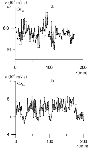
Figure 1: Time dependences of kinematic viscosity of liquid copper [9, 10](a) and liquid cobalt (1870 K) [8] (b) close to the temperature of step change of viscosity.

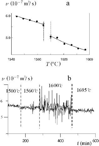
Figure 2: Temperature dependence of kinematic viscosity of liquid cobalt (a) and time dependence’s of liquid cobalt viscosity at various temperatures (b).

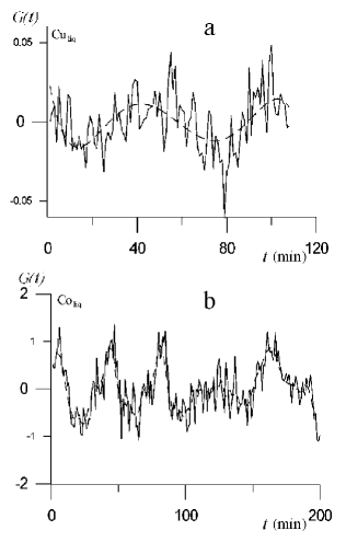
Figure 3: Time dependences of autocorrelation function for the liquid copper (a), and liquid cobalt (b) viscosity close to corresponding temperatures of step change of viscosity.

Besides, there are facts, which suggest that the process of establishing a thermodynamic equilibrium in the system close to this point can have a non-monotonic oscillating character [6]. This effect was observed on the polytherms of viscosity, surface tension and magnetic susceptibility of metal melts, and the low-frequency modes $\omega\sim 10^{-2}$ $s^{-1}$ predominated in these oscillations [6, 7] several times. For example, the time dependence of the kinetic viscosity of liquid Co at $T=1600$ ^∘C is presented in Fig.1(b). These results were obtained in [8] by the torsional vibrations method in isothermal regime. As usual [8], the temperature was rapidly elevated and maintained at the given level. In the figure one can see considerable fluctuating of the measured quantities of viscosity. They have a stochastic character, and their amplitude exceeds the experimental error. It is important that the system temperature is close to the point of the step change of viscosity (Fig.2). The dispersion of viscosity values in this point considerably exceeds the dispersions of viscosity values at other temperatures. The usual variation of viscosity is $\Delta\nu\sim 0.7\cdot 10^{-7}$ m${}^{2}/$s for discussed experiments, but this dispersion grows by 3–4 times near the vicinity of the temperature at which the viscosity polytherms jump are observed. The spectral-correlation analysis of these data was shown in the following papers [9, 10]. The results have confirmed the supposition that a pronounced low-frequency mode is present in these data (Fig.3).

Unfortunately, so far, the reliability of the above data has been questionable and true conclusions about the character and mechanism of the observed relaxation processes have remained unsolved. It is connected with the difficulties of developing specific precise experimental techniques and processing the obtained data as well as with the lack of the appropriate theoretical models. However, it is natural to suppose that these effects can be generated by some local structure modifications. Since the oscillation relaxation processes are observed in the neighborhood of the step change of liquid viscosity we believe these effects to be connected with each other. Besides these vibrations look like as a fluctuations reinforcement near the phase transition point (Fig.2). Therefore in this paper we assume that liquid–liquid transition point is root of both the step change of liquid viscosity and the oscillating relaxation.

2 THEORETICAL MODEL

It is known that thermodynamic systems are metastable at the temperatures close to critical ones. This metastability can be described by addition of the non-linear part to non-equilibrium thermodynamic potentials of the system. On the other hand, such systems undergo strong thermodynamic fluctuations as well as the effect of external ”noise” because of both the influence of the experimental plant and thermal fluctuations. Thus, one can suppose that the combination of strong none-linearity of the metastable system and fluctuations is the reason of the oscillating relaxation, but the nature of metastability is clear only in the case of melts, whereas the nature of the liquid–liquid transition in liquid metals is still unclear. Therefore, we think, that the problem of theoretical description of the oscillating relaxation is reduced to two problems: first of all, it is necessary to define the nature of the liquid–liquid transition in the metal liquid and give its theoretical model. After that one can discuss the dynamic peculiarity of this model, and the chance of appearance of the low frequency mode in the oscillation spectrum.

In most of theoretical papers liquid is treated as the one consisting of adjoining to each other and interacting with each other elementary local volumes which include atoms of several coordination spheres [11, 12, 13, 14]. It is expected that each of these local volumes has only a few energy–profitable configurations of the nearest order (local states). The long-range order is absent here as the local groups of atoms can be oriented differently with respect to each other. The topological structures of these locally–ordered formations have some symmetry. One can suppose that this local symmetry corresponds either to the crystal symmetry (solid-like), e.g. f.c.c. or b.c.c., or to the icosahedral symmetry (normal-liquid). We believe that as the temperature decreases both normal-liquid and solid-like locally favored structures (LFS) [11] can form clusters. These clusters have a finite size and continuously transform, since the thermal fluctuations of the system lead to continuous destroying old bonds and to simultaneous forming new ones.

Let us consider the case when the temperature of the melt is close to that of the liquid–liquid transition. The foolproof theory of the structural transitions in liquids is not available for the time being. Therefore to describe the metastable properties of the close to this transition system we will consider the simplest model. As well as it was in [11] we will describe the close to liquid-liquid transition system as the system that is near the gas–liquid transition. We believe that the order parameter is connected with density. Therefore, using the density as the order parameter we introduce the following free energy, which governs $\psi$ fluctuations near the gas–liquid-like critical point $T_{cr}$ [15]:

$$F_{0}=\displaystyle\frac{1}{2}\int d^{d}x\left[\;(\vec{\nabla}\psi)^{2}+\gamma(T,\,P)\psi+\alpha(T-T_{cr})\psi^{2}+\frac{g}{2}\psi^{4}\;\right],$$ (1)

$\gamma(T,\,P)$ is the function of temperature $T$ and pressure $P$, the parameters $g$ and $\alpha$ are weakly depending on temperature.

3 DESCRIPTION OF THE RELAXATION

Let us consider the fluctuations of the order parameter of metastable liquid in the region of phases co-existence ($\gamma\approx 0$). In order to describe the relaxation dynamics of this system we will consider the H-model [19]. This model is represented by the following equations system:

$$\begin{array}[]{c}\displaystyle\frac{\displaystyle\partial\psi}{\displaystyle\partial t}=\displaystyle\lambda\nabla^{2}\frac{\displaystyle\delta F}{\displaystyle\delta\psi}-g_{0}\vec{\nabla}\psi\cdot\frac{\displaystyle\delta F}{\displaystyle\delta\vec{v}}+\theta,\\[12.0pt] \displaystyle\frac{\displaystyle\partial\vec{v}}{\displaystyle\partial t}=\displaystyle P^{\perp}\left[\;\eta_{0}\nabla^{2}\frac{\displaystyle\delta F}{\displaystyle\delta\vec{v}}+g_{0}\vec{\nabla}\psi\frac{\displaystyle\delta F}{\displaystyle\delta\psi}+\vec{\xi}\;\right],\\[12.0pt] F=\displaystyle F_{0}-\int d^{d}x\left[\;h(\vec{x},\,t)\psi+\vec{A}(\bar{x},\,t)\cdot\vec{v}\;\right],\\[10.0pt] F_{0}=\displaystyle\frac{1}{2}\int d^{d}x\left[\;\tau\psi^{2}+(\vec{\nabla}\psi)^{2}+\frac{g}{2}\psi^{4}+\vec{v}^{2}\;\right],\end{array}$$ (2)

where $\tau=\alpha(T-T_{cr})$, $h$ and $\vec{A}$ are infinitesimal applied fields. The first equation describes the dynamics of the order parameter $\psi$, and the second one describes the dynamics of the transverse part of the momentum density $v$, ($P^{\perp}$ is a projection operator which selects the transverse part of the vector in brackets, $\lambda$ is the coefficient of self-diffusion, $\eta_{0}$ is the viscosity, $g_{0}=\left.1\right/\lambda\eta_{0}$ is the mode-coupling vertex, the functions $\vec{\xi}$ and $\theta$ are the Gaussian white noise source:

$$\begin{array}[]{c}\langle\theta(x,\,t)\theta(x^{\prime},\,t^{\prime})\rangle=-\lambda\nabla^{2}\delta(x-x^{\prime})\delta(t-t^{\prime}),\\[12.0pt] \langle\xi_{i}(x,\,t)\xi_{j}(x^{\prime},\,t^{\prime})\rangle=-\eta_{0}\nabla^{2}\delta(x-x^{\prime})\delta(t-t^{\prime})\delta_{ij}.\end{array}$$

The critical properties of this model are known [19]. In particular, it is well known that the viscosity of such a system depends on the character time of the experiment $t_{ch}=1/{\omega_{ch}}$. In the case of the results discussed above, this quantity is the frequency of torsional vibrations. Therefore, one can really expect that the change of the viscosity around $T_{cr}$ will be prolonged in some temperature interval $T_{1}>T>T^{*}(\omega)$ rather than jump-like ($T_{1}$ is the temperature of formation of the metastable phase). It agrees with the experimental observations. Note, that this interval depends on the frequency of torsional vibrations $\omega$:

$$T^{*}(\omega)-T_{cr}\sim\left(\frac{\displaystyle\omega}{\displaystyle\lambda}\right)^{\left.1\right/(\nu z)}$$ (4)

($\nu$ and $z$ are corresponding static and dynamic critical exponents). At the low-frequency $\omega<1/t_{cl}$ ($t_{cl}$ is the life-time of the clusters ) the value of viscosity $\eta(\omega)$ will be slightly dependent on the correlation length $\xi_{c}$ (clusters size). But at the higher frequency $\omega\gg 1/t_{cl}\sim\xi_{c}^{-z}$ the response to the mechanical perturbation will be determined by the scale which is smaller than the cluster size, and it will not depend on the frequency.

4 THEORETICAL EXPLANATION OF THE VISCOSITY TIME OSCILLATING

Usually model (2) is used for theoretical description of critical dynamics of gas-liquid transitions and transitions in binary fluids. The system inertia is not taken into account. The point is, the critical dynamics is usually investigated, and in this case the rescaling operator increases the importance of $\omega$, relative to $\rho\omega^{2}$, and after the renormalization procedure the term $\rho\omega^{2}$ may be neglected. However, we will investigate the nonlinear stochastic system which is not found correct at the critical point. In this case the non-linearity of the system can lead to the state when even its weak inertia will essentially influence long-time dynamics [20]. In order to take it into account, it is necessary to add the proportional to double $t$-derivation term to the first equation of the system:

$$\displaystyle\rho\frac{\displaystyle\partial^{2}\psi}{\displaystyle\partial t^{2}}+\frac{\displaystyle\partial\psi}{\displaystyle\partial t}=\displaystyle\lambda\nabla^{2}\frac{\displaystyle\delta F}{\displaystyle\delta\psi}-g_{0}\vec{\nabla}\psi\cdot\frac{\displaystyle\delta F}{\displaystyle\delta\vec{v}}+\theta.$$

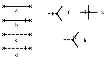
Figure 4: Graphs $a,b,c,d$ correspond to propagators $<\psi\psi>$, $<\psi\psi^{\prime}>$, $<vv>$, and $<vv^{\prime}>$ accordingly, graphs $f,g,h$ correspond to vertexes $v^{\prime}\psi\partial(\partial^{2}\psi)$, $\lambda g\psi^{\prime}\partial^{2}(\psi^{3})$, and $\psi^{\prime}v\partial\psi$ accordingly.

To analyze this stochastic model, one can employ the standard method of the stochastic deriving functional [21] and theory of perturbation. According to these methods, the correspondent field model will be described by a set of basic $\{\psi,\,v\}$ and supplementary $\{\psi^{\prime},\,v^{\prime}\}$ fields, and the effective action will have the form (Fig.4) of:

$$\begin{array}[]{rcl}S(\Phi)&=&-\lambda\psi^{\prime}\partial^{2}\psi^{\prime}+\psi^{\prime}[-\rho\partial_{t}^{2}\psi-\partial_{t}\psi-\lambda\partial^{2}(\partial^{2}\psi-\tau\psi-\gamma\psi^{2}-g\psi^{3})-\\[12.0pt] &-&v\partial\psi]+\lambda^{-1}g_{0}^{-1}v^{\prime}\partial^{2}v^{\prime}+v^{\prime}[-\partial_{t}v+\lambda^{-1}g_{0}^{-1}\partial^{2}v+\psi\partial(\partial^{2}\psi)].\end{array}$$

The propagators of fields $\psi$ and $v$ have the form of:

$$\begin{array}[]{c}\displaystyle\langle\psi\psi^{\prime}\rangle=\langle\psi^{\prime}\psi\rangle^{T}=\displaystyle\frac{\displaystyle 1\left/\rho\right.}{\displaystyle-\omega^{2}-ia\omega+\varepsilon_{k}},\quad\langle\psi\psi\rangle=\frac{\displaystyle 2\lambda k^{2}\left/\rho^{2}\right.}{\displaystyle\left(-\omega^{2}-ia\omega+\varepsilon_{k}\right)\left(-\omega^{2}+ia\omega+\varepsilon_{k}\right)},\\[12.0pt] \displaystyle\langle vv^{\prime}\rangle=\langle v^{\prime}v\rangle^{T}=\displaystyle\frac{\displaystyle\lambda g_{0}P^{\perp}}{\displaystyle-i\omega\lambda g_{0}+k^{2}},\qquad\langle vv\rangle=\frac{\displaystyle 2\lambda g_{0}k^{2}}{\displaystyle\left(-i\omega\lambda g_{0}+k^{2}\right)^{2}},\end{array}$$

where

$$\displaystyle\varepsilon_{k}=\frac{\displaystyle\lambda}{\displaystyle\rho}\,k^{2}(k^{2}+r_{0}),\qquad a=\frac{\displaystyle 1}{\displaystyle\rho}\,,$$

and $r_{0}$ is a renormalized quantity $\tau$, $k^{2}$ is the impulse $\vec{k}$ squared. Below we will consider only the propagators of the conservative order parameter field $\psi$. For calculation it is convenient to use the $(k,\,t)$-representation, in this case, the propagators become:

$$\begin{array}[]{rl}&\displaystyle\langle\psi\psi^{\prime}\rangle=\frac{\displaystyle 2\pi\,e^{-\left.at\right/2}}{\displaystyle\rho\sqrt{-4\varepsilon_{k}+a^{2}}}\exp\left(-\frac{\displaystyle 1}{\displaystyle 2}\sqrt{-4\varepsilon_{k}+a^{2}}|t|\right),\\[12.0pt] &\displaystyle\langle\psi\psi\rangle=\frac{\displaystyle\lambda\pi k^{2}}{\displaystyle a\rho^{2}\varepsilon_{k}}\,\exp\left(-\frac{\displaystyle 1}{\displaystyle 2}\sqrt{-4\varepsilon_{k}+a^{2}}|t|\right)\left[\frac{\displaystyle e^{\left.a|t|\right/2}}{\displaystyle\sqrt{-4\varepsilon_{k}+a^{2}}}\left(\sqrt{-4\varepsilon_{k}+a^{2}}+a\right)-\right.\\[12.0pt] &\displaystyle-\left.\frac{\displaystyle e^{-\left.a|t|\right/2}}{\displaystyle\sqrt{-4\varepsilon_{k}+a^{2}}}\left(\sqrt{-4\varepsilon_{k}+a^{2}}-a\right)\right],\end{array}$$

when $4\varepsilon_{k}<a^{2}$, and

$$\begin{array}[]{rl}&\displaystyle\langle\psi\psi^{\prime}\rangle=\frac{\displaystyle 2\pi\,e^{-\left.at\right/2}}{\displaystyle\rho\sqrt{4\varepsilon_{k}-a^{2}}}\sin\left(\frac{\displaystyle 1}{\displaystyle 2}\sqrt{4\varepsilon_{k}-a^{2}}\,\,t\right)\left[\theta(t)-\theta(-t)\right],\\[14.0pt] &\displaystyle\langle\psi\psi\rangle=\frac{\displaystyle\lambda\pi k^{2}}{\displaystyle a\rho^{2}\varepsilon_{k}}\frac{\displaystyle\left[\theta(t)-\theta(-t)\right]}{\displaystyle\sqrt{4\varepsilon_{k}-a^{2}}}\left[e^{-\left.at\right/2}\left\{\sqrt{4\varepsilon_{k}-a^{2}}\cos\left(\frac{\displaystyle 1}{\displaystyle 2}\sqrt{4\varepsilon_{k}-a^{2}}\,\,t\right)+\right.\right.\\[14.0pt] &\displaystyle\left.+a\sin\left(\frac{\displaystyle 1}{\displaystyle 2}\sqrt{4\varepsilon_{k}-a^{2}}\,\,t\right)\right\}+\,e^{\left.at\right/2}\left\{a\sin\left(\frac{\displaystyle 1}{\displaystyle 2}\sqrt{4\varepsilon_{k}-a^{2}}\,\,t\right)-\right.\\[14.0pt] &\displaystyle\left.\left.-\sqrt{4\varepsilon_{k}-a^{2}}\cos\left(\frac{\displaystyle 1}{\displaystyle 2}\sqrt{4\varepsilon_{k}-a^{2}}\,\,t\right)\right\}\right],\end{array}$$

when $4\varepsilon_{k}>a^{2}$. It is important that the effective viscosity depends on $\omega$, and it can be represented as

$$\eta(\tau,\,\omega)=\displaystyle\eta_{0}\left[1-\frac{\displaystyle\displaystyle\lambda g_{0}\Sigma_{v^{\prime}v}}{\displaystyle\displaystyle p^{2}}\right],$$

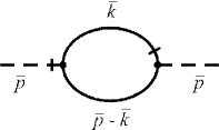
Figure 5: The graph corresponds to the response function $\Sigma_{v^{\prime}v}$ in the framework one-loop approximation.

where $\Sigma_{v^{\prime}v}$ is a coupled-mode contribution to the response function, $\vec{p}$ is an external impulse. In an one-loop approach it can be represented in the diagram form (Fig.5), in mathematic $(k,\,t)$-representation this contribution has the form of:

$$\begin{array}[]{rcl}\Sigma_{v^{\prime}v}(t,\,p)&=&\displaystyle\frac{\displaystyle\pi^{2}}{\displaystyle a\rho^{2}}\displaystyle\int\frac{\displaystyle d^{3}k}{\displaystyle(2\pi)^{3}}\frac{\displaystyle[k_{i}P_{ij}^{\perp}k_{j}][p^{2}-2\vec{p}\cdot\vec{k}]}{\displaystyle[q^{2}+r_{0}]\sqrt{-4\varepsilon_{k}+a^{2}}}\exp\left(-|t|\left[\sqrt{-4\varepsilon_{q}+a^{2}}+\sqrt{-4\varepsilon_{k}+a^{2}}\right]\right)\times\\[12.0pt] &\times&\displaystyle\left[\frac{\displaystyle a}{\displaystyle\sqrt{-4\varepsilon_{q}+a^{2}}}\left(1+e^{-at}\right)+\left(1-e^{-at}\right)\left(\theta(t)-\theta(-t)\right)\right],\qquad(\bar{q}=\bar{p}-\bar{k}),\end{array}$$

in case of $4\varepsilon_{k}<a^{2}$, and

$$\begin{array}[]{rcl}\Sigma_{v^{\prime}v}(t,\,p)&=&\displaystyle\frac{\displaystyle\pi^{2}}{\displaystyle a\rho^{2}}\displaystyle\int\frac{\displaystyle d^{3}k}{\displaystyle(2\pi)^{3}}\frac{\displaystyle[k_{i}P_{ij}^{\perp}k_{j}][p^{2}-2\vec{p}\cdot\vec{k}]}{\displaystyle[k^{2}+r_{0}]\sqrt{(4\varepsilon_{q}-a^{2})(4\varepsilon_{k}-a^{2})}}\left[\theta(t)-\theta(-t)\right]\sin\left(\frac{\displaystyle 1}{\displaystyle 2}\sqrt{4\varepsilon_{q}-a^{2}}\,t\right)\times\\[12.0pt] &\times&\displaystyle\left[e^{-at}\left\{\sqrt{4\varepsilon_{k}-a^{2}}\cos\left(\frac{\displaystyle 1}{\displaystyle 2}\sqrt{4\varepsilon_{k}-a^{2}}\,\,t\right)+a\sin\left(\frac{\displaystyle 1}{\displaystyle 2}\sqrt{4\varepsilon_{k}-a^{2}}\,\,t\right)\right\}+\right.\\[14.0pt] &&\displaystyle+\left.\left\{a\sin\left(\frac{\displaystyle 1}{\displaystyle 2}\sqrt{4\varepsilon_{k}-a^{2}}\,\,t\right)-\sqrt{4\varepsilon_{k}-a^{2}}\cos\left(\frac{\displaystyle 1}{\displaystyle 2}\sqrt{4\varepsilon_{k}-a^{2}}\,\,t\right)\right\}\right],\\[12.0pt] &&(\bar{q}=\bar{p}-\bar{k}),\end{array}$$

in case of $4\varepsilon_{k}>a^{2}$. If we switch from integration at $k$ to integration at $\omega=\sqrt{4\varepsilon_{k}-a^{2}}$ in limit $t\to\infty$ and $p\to 0$ we can obtain:

$$\displaystyle\lim_{p\to 0}\frac{\displaystyle\Sigma_{v^{\prime}v}(t,\,p)}{\displaystyle p^{2}}=\frac{\displaystyle\left(\rho\lambda\right)^{-3/4}}{\displaystyle 16\sqrt{2}a}\int d\omega\left[f_{1}(\omega)\sin(\omega t)+f_{2}(\omega)(\cos(\omega t)+1)\right],$$

where

$$\begin{array}[]{c}\displaystyle f_{1}(\omega)=\frac{\displaystyle\left(-r_{0}\sqrt{\lambda\rho}+\sqrt{\lambda\rho r_{0}^{2}+w^{2}\rho^{2}+1}\,\right)^{3/2}}{\displaystyle\left(r_{0}\sqrt{\lambda\rho}+\sqrt{\lambda\rho r_{0}^{2}+w^{2}\rho^{2}+1}\right)\sqrt{\lambda\rho r_{0}^{2}+w^{2}\rho^{2}+1}}\,,\qquad f_{2}(\omega)=\frac{\displaystyle f_{1}(\omega)}{\displaystyle\rho\omega}\,.\par\end{array}$$

Fig.6 shows the qualitative aspect of this spectrum. One can see tow peaks in this figure. The $\omega=0$ peak corresponds to the Goldstone mode and it is explained by the presence of preservation law for $\psi$ and $v$. Another peak

$$\omega\simeq\frac{\displaystyle 1}{\displaystyle\rho}\sqrt{1-\frac{\displaystyle 68.4\lambda\rho}{\displaystyle\xi_{c}^{4}}}$$

corresponds to the low-frequency oscillations of the system. Thus, it is possible to conclude that the observed oscillations are noise-induced, analogous to the noise-induced oscillations in bistable systems, and excitation of the low-frequency modes in the system can be a noise-induced transition [22] (non-equilibrium phase transition).

Then the condition of observation of these oscillations is $\xi_{c}\approx\displaystyle\left[68.4\lambda\rho\right]^{\frac{1}{4}},$ and one can estimate the correlation length quantity: Since $\lambda=D_{a}a_{0}^{2}$, where $D_{a}\sim 10^{-9}$ $\left.m^{2}\right/s$ is the diffusion coefficient, $a_{0}\sim 10^{-9}$ $m$ is the interatomic distance, and $\rho$ is the relaxation time, we believe that these values are of the order of the torsional vibration period (it is $\rho\sim 1$ $s$ in our experiments [8]). Then the correlation length is $\xi_{c}\sim 10^{-7}$ $m$. One can anticipate that it is the size of the flickering clusters of the metastable phase. It should be noted that this value is close to the size of the ”Fischer clusters” which was observed in supercooled liquids [3], but direct observation of these formations at the relatively high temperatures is not available for the time being.

5 CONCLUSIONS

It is well known that liquid is a nonuniform system, and its structure is characterized by the presence of the structure clusters in it. Recently the polymerization-like processes have been observed in metal systems by small-angle neutrons dispersion experiments [3]. In these experiments the snowflake-like large-size heterogeneity was discovered. We believe that similar processes of liquid–liquid transition lead to appearance of structured fluid (rheology) properties in liquids at relatively low temperatures, and to the jumps in the viscosity polytherms of some liquid metals.

In an attempt to explain the observed oscillations of viscosity, we assume that presence of liquid–liquid transition point is the possible root of appear of the properties oscillating in the explored systems. We believe that they are caused by the exterior noise. Nonlinearity of the system in the region of its metastability is the reason of the increase of the fluctuations dispersion, and the possible reason of the oscillating character of these fluctuations. The latter is caused by the low-frequency peak in the spectrum, and we believe that this effect analogous to well-known noise-induced transitions in bistable systems [22]. We would like to mark that one ought not to consider the period of the viscosity oscillation as a life time of the metastable subsystems (clusters). The sizes of the such subsystems are about correlation radius $\sim\xi_{c}$ and their fluctuations frequency is a reciprocal value for the lifetime $t_{cl}\sim\xi_{c}^{z}\sim 10^{-10}$ s. As indicated above the viscosity oscillation is the dynamic effect, which is determined by influence of the fluctuating moving to the hydrodynamic moving, and inheres in the whole system.

Further examination of nontrivial dynamic properties of such systems will allow us to confirm or discard our hypothesis.

This study was supported by the RFBR grant (01-02-96455 r2001ural).

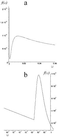
Figure 6: The spectrum of viscosity oscillations ($f(\omega)=\sqrt{f_{1}(\omega)^{2}+f_{2}(\omega)^{2}}$) in linear–linear (a) and logarithmic–linear (b) coordinates.

References

- [1] Y. Katayama, T. Mizutani, W. Utsumi et al, “A first-order liquid–liquid phase transition in phosphorus,” Nature, 403, 170–173 (2000);
- [2] J.N. Glosli and F.H. Ree, “Liquid–liquid phase transition in carbon,” Phys. Rev. Lett. 82, 4659 (1998);
- [3] U. Dahlborg, M. Calvo-Dahlborg, P. Popel, and V. Sidorov, “Structure and properties of some glass-forming liquid alloys,” Eur. Phys. J. B. 14, p. 639–648 (2000);
- [4] G. Franzese, G. Malescio, A. Skibinsky, S.V. Buldyrev and H.E. Stanley, “Generic mechanism for generating a liquid–liquid phase transition,” Nature, 409, 692–695 (2001);
- [5] V.I. Lad’yanov, A.L. Bel’tyukov, K.G. Tronin, and L.V. Kamaeva, “Structural transition in liquid cobalt,” Pisma. Zh. Eksp. Teor. Fiz. 72, 6, 436–439 (2000) [JETP Letters, 72, 6, 301–303 (2000)];
- [6] B.A. Baum, I.N. Igoshin, D.B. Shulgin et al, “On oscillating character of the relaxation process of non-equilibrium metal melts,” Rasplavy (in Russian) 2, 5, 102–105 (1988);
- [7] V.I. Lad’yanov, S.V. Logunov, and S.V. Pakhomov, “On oscillating relaxation processes in non-equilibrium metal melts after melting,” Rasplavy (in Russian), 5, 20–23 (1998);
- [8] V.I. Lad’yanov, A.L. Bel’tyukov, M.G. Vasin, and L.V. Kamaeva, “About structural transition and time-unstability in liquid cobalt,” Rasplavy (in Russian), 1, 32–39 (2003);
- [9] M.G. Vasin, V.I. Lady’anov, and V.P. Bovin, “About the mechnism of the non-monotonic relaxation processes in metal fluids,” Metally (in Russian), 5, 27–32 (2000);
- [10] V.I. Lad’yanov, M.G. Vasin, S.V. Logunov, and V.P. Bovin, “Nonmonotonic relaxation processes in nonequilibrium metal melts,” Phys. Rev. B1 62, 18, 12107–12112 (2000);
- [11] H. Tanaka, ”General view of a liquid–liquid phase transition,” Phys. Rev. E 62, 5, 6968–6976 (2000);
- [12] A.Z. Patashinski, and A. C. Mitus, “Towards understanding the local structure of liquids,” Phys. Repts. 288, 1–6, 409–434 (1997);
- [13] L.D. Son, and G.M. Rusakov, “The model of the phase transition in the melt,” Rasplavy (in Russian), 5, 90–95 (1995);
- [14] A.S. Bakai, “Long-range density fluctuations in the glass-forming liquids,” J. Non-Cryst. Solids. 307–310, 623–629 (2000);
- [15] Yu.L. Klimontovich, Statisticheskaya Fizika (Statistical Physics), Harwood Academic Publ., New York: 1986;
- [16] V.V. Brazhkin, R.N. Voloshin, A.G. Lyapin, and S.V. Popova, “Quasi-transitions in simple liquids at high pressures,” Uspekhi Phizicheskikh Nauk 169, 9, 1035–1039 (1999);
- [17] E.W. Fischer, “Light Scattering and Dielectric Studies on Glass Forming Liquids,” Physica A 201, 183–206 (1993);
- [18] De Gennes P.G., Scaling Concepts in Polimer Physics, L.: Pergamon Press, 1983, 279 p.;
- [19] P.C. Hohenberg and B.I. Halperin, “Theory of dynamic critical phenomena,” Rev. Mod. Phys. 49, 435–479 (1977);
- [20] W. Coffey, M. Evans, and P. Grigolini, Molecular Diffusion and Spectra. Moscow.: Mir, 1987, 384 p.;
- [21] A.N. Vasiliev, The quantum-field renormalization-group method in theory of critical behaviour and stochastic dynamics, PNPI Press, S–Petersburg, ISBN 5-86763-122-2, 1998, 774 p.;
- [22] W. Horsthemke, and R. Lefever, Noise-Induced Transitions: Theory and Applications in Physics, Chemistry, and Biology, Springer–Verlag, Berlin, Heidelberg, New York, Tokyo: 1984;
- [23] L.D. Son, and B.E. Sidorov, “Polymerization in glass-forming melts,” Izvestia academii nauk (in Russian) 65, 10, 1431–1434 (2001).