Persistent spin current and entanglement in the anisotropic spin ring

Abstract

We investigate the ground state persistent spin current and the pair entanglement in one-dimensional antiferromagnetic anisotropic Heisenberg ring with twisted boundary conditions. Solving Bethe ansatz equations numerically, we calculate the dependence of the ground state energy on the total magnetic flux through the ring, and the resulting persistent current. Motivated by recent development of quantum entanglement theory, we study the properties of the ground state concurrence under the influence of the flux through the anisotropic Heisenberg ring. We also include an external magnetic field and discuss the properties of the persistent current and the concurrence in the presence of the magnetic field.

I introduction

Transport properties of strongly correlated systems have attracted great theoretical and experimental interest for more than two decades. In particular, low-dimensional systems show significant deviations in transport properties from the usual Fermi-liquid quasiparticle description. It has been revealed that electron correlation and topology play important roles in one-dimensional systems. Recently, the study of transport properties in integrable models has been an active field of research. The two most studied models are the hubbard model and the spinless fermion(or, equivalently, spin-1/2 Heisenberg chain) model. Several experiments LPLevy ; VChandrasekhar ; DMailly ; BReulet ; EMQJariwala ; WRabaud have observed persistent currents in mesoscopic metallic and semiconducting rings pierced by a magnetic flux. These studies have led to many theoretical investigations focusing on the interplay of electron-electron interaction and disorder in such systems. The persistent current in a ferromagnetic Heisenberg ring has been studied in crown-shaped magnetic field FlorianSchutz , which can also be driven by an inhomogeneous electric fields ZLCao due to the Aharonov-Casher effect YAharonov . Based on a spin-wave approach, the spin current in an antiferromagnetic Heisenberg ring with integer spin in an inhomogeneous magnetic field has been investigated very recently F. Schutz .

In the first part of this paper we study the ground state persistent current of a spin-1/2 anisotropic Heisenberg spin ring pierced by a flux. By solving Bethe ansatz equations numerically, we find that the increasing anisotropy reduces the amplitude of the persistent current. This phenomenon has also been noticed by G.Bouzerar Bouzerar using the Lanczos method. We also study the influence of an external magnetic field on the ground-state persistent current, and find that the increasing magnetic field reduces the amplitude of the persistent current. When the magnetic field is larger than a certain value ($h=3.0$ for $\Delta=0.5$, when the spins are fully polarized), the persistent current vanishes.

Quantum entanglement, as exemplified in the singlet state of two spin-1/2 particles $(1/\sqrt{2})(|\uparrow\downarrow>-|\downarrow\uparrow>)$, is a correlation between two quantum subsystems. It bears some resemblance to classical correlation, but differs in important aspects, highlighted by the observation of the violation of Bell’s inequalities in entanglement systems. For a special case of three binary quantum objects(three qubits), a quantitative extension of these inequalities has been proposed in terms of a measure of the entanglement called the “concurrence”, which takes values between zero and one. Several theoretical studies CHBennett ; SHill ; wootters have pointed out, for example, that the square of the concurrence between qubits A and B, plus the square of the concurrence between A and C, cannot exceed unity VCoffman . Meanwhile, it has been found experimentally that entanglement is crucial to describe magnetic behavior in a quantum spin system Ghose . Therefore, we hope that the study of the entanglement in Heisenberg models will enhance our understanding of the quantum features of magnetic systems.

We may regard a spin-1/2 chain as a collection of interacting qubits. This connection has motivated us to carry out the second part of the study to investigate the entanglement in anisotropic spin chains. There have already been several studies on the entanglement in spin chains MCArnesen ; DGunlycke ; wangPRA ; GLagmago ; YangSun ; LFSantos ; TJOsborne . In particular, recent efforts KMOConnor ; VBuzek ; sjgu2005 ; ClareDunning have been made to understand the quantum entanglement in the ground states of some many-body models, in the hope that the study of entanglement can provide a new insight into the quantum phase transition AOsterloh ; GVidal in these systems. Motivated by a recent work about the entanglement generation in persistent current qubits JFRalph . To this end, we study the properties of the ground state concurrence and its connections with persistent current. Our numerical results show that the concurrence is a periodic function of $\phi$. The locations of the minimum concurrence correspond to those of the maximum persistent current where an energy level crossing occurs. In the presence of the external magnetic field, the concurrence increases with the magnetic field, though the minima become less sharp as the magnetic field increases.

II the model and its secular equation

The Hamiltonian of an anisotropic Heisenberg ring with twisted boundary conditions reads:

$$H=-J\sum\limits_{l=1}^{N}{\left[\frac{1}{2}(S_{l}^{+}S_{l+1}^{-}e^{-i\phi/N}+H.c.)+\Delta S_{l}^{z}S_{l+1}^{z}\right]}$$ (1)

where $N$ is the number of sites. The total magnetic flux, or the Aharonov-Bohm flux, through the ring is $\Phi$, and $\phi=2\pi\Phi/\Phi_{0}$ where $\Phi_{0}=hc/e$ is the flux quantum. $S_{l}^{+}$, $S_{l}^{-}$, and $S_{l}^{z}$ are spin-1/2 operators at site $l$. By using Wigner-Jordan transformation Jordan , the Hamiltonian Eq. (1) can be mapped to a spinless fermion model:

$$H=-\frac{J}{2}\sum\limits_{i}({C_{i}^{+}}C_{i+1}e^{-i\phi/N}+{C_{i+1}^{+}}C_{i}e^{i\phi/N})$$

$$+V\sum\limits_{i}{(\hat{n}_{i}-\frac{1}{2})(\hat{n}_{i+1}-\frac{1}{2})},$$ (2)

where $J/2$ can be interpreted as the hopping integral and $V=J\Delta$ as the nearest-neighbor Coulomb repulsion. The spinless fermionic operators $c_{i}^{+}$ and $c_{i}$ obey the anticommutation relations, and $\hat{n}_{i}=c_{i}^{+}c_{i}$ is the local number operator. It is well known that the ground state of this model has different phases: a metallic phase when $0<\Delta<1$ and an insulating phase when $\Delta>1$, where $\Delta$ is the anisotropy, or interaction. The former phase is gapless while the latter gapful.

As in Ref. Li , the flux can be gauged out of the Hamiltonian Eq. (1), so that solving the Schrödinger equation in the presence of a magnetic flux with a periodic boundary condition is equivalent to that in the absence of the flux but with a twisted periodic condition, namely,

$$\psi(x_{1},\cdots x_{i}+L,\cdots)=\exp(i\phi)\psi(x_{1},\cdots x_{i},\cdots).$$ (3)

We emphasize that the characteristic length $L$ of the circumference is a mesoscopic scale so that inelastic scattering does not occur. This justifies the applicability of the Bethe ansatz approach for the present problem, because the ansatz embodies nondiffractive scattering.

From the standard quantum inverse scattering methods (QISM) HABethe ; takahashi , the diagonalization of Hamiltonian Eq. (1) can be transformed into solving the following Bethe ansatz equations:

$$\left({\frac{{\sinh\frac{\gamma}{2}(x_{j}+i)}}{{\sinh\frac{\gamma}{2}(x_{j}-i)}}}\right)^{N}=e^{-i\phi}\prod\limits_{l\neq j}^{M}{\frac{{\sinh\frac{\gamma}{2}(x_{j}-x_{l}+2i)}}{{\sinh\frac{\gamma}{2}(x_{j}-x_{l}-2i)}}},$$ (4)

where $\gamma$ satisfies $\Delta=\cos(\gamma)$.

Taking the logarithm of Eq. (4), we obtain

$$N\theta_{1}(x_{j},\gamma)=2\pi I_{j}+\phi+\sum\limits_{l=1}^{M}{\theta_{2}(x_{j}-x_{l},\gamma)},$$ (5)

where

$$\theta_{n}(x,\gamma)=2\tan^{-1}[\frac{{\tanh(\gamma x/2)}}{{\tan(n\gamma/2)}}].$$

The ground state is described by a symmetrical sequence of quantum numbers around zero. They are

$$I_{j}=\{-\frac{{M-1}}{2},-\frac{{M-3}}{2},...,\frac{{M-1}}{2}\}.$$

The energy of the ground state can be expressed as:

$$E=E_{0}-J\sum\limits_{j=1}^{M}{\frac{{\sin^{2}(\gamma)}}{\cosh(\gamma x_{j})-\cos(\gamma)}}.$$ (6)

In the thermodynamics limit, it can be written in an integral form,

$$E=E_{0}-JN\sin^{2}\gamma\int{{{\rho_{N}(x,\phi)dx}\over{\cosh(\gamma x)-\cos\gamma}}}$$

$$\times\sum\limits_{m=-\infty}^{\infty}{\exp\{im[Np_{N}(x)-\phi]\}},$$ (7)

where $p_{N}(x_{i})=(2\pi I_{i}+\phi)/N$ and $E_{0}=J\Delta N/4$.

At $T=0$, the equilibrium persistent current can be given by $I(\phi)=-(e/\hbar)\partial E(\phi)/\partial\phi$, where $E(\phi)$ is the ground-state energy of Eq. (1), as a function of the boundary condition $\phi$ [Eq. (3)].

III persistent spin current

To obtain the ground state of the anisotropic Heisenberg model, which is a spin singlet state $(N=2M)$, we solve the Bethe ansatz equations Eq. (5) at zero temperature and calculate the dependence of the ground-state energy on flux. From the Eq. (5), we find that when $\phi<\pi$, the quantum number sequence of the lowest energy state should be the same as the ground state when $\phi=0$. But if $\pi<\phi<3\pi$, the quantum number sequence of the lowest energy state should be $I_{j}=\{-\frac{{M+1}}{2},-\frac{{M-1}}{2},...,\frac{{M-3}}{2}\}$. Likewise, for $3\pi<\phi<5\pi$, it should be $I_{j}=\{-\frac{{M+3}}{2},-\frac{{M+1}}{2},...,\frac{{M-5}}{2}\}$. In other words, when $\phi$ reaches $(2n+1)\pi$, there is an energy level crossing at the lowest energy level. As the flux increased, the original ground-state energy increases while excited energy decreases. They are the same when $\phi$ equals $(2n+1)\pi$. Here we solve a system with 42 spins, and obtain the ground state energy as in Fig. (1).

Figure 1: The ground state energy of anisotropic Heisenberg spin ring as a function of flux when $\Delta=0.5403$.

We can find that the ground state energy is a periodic function with respect to the flux, with a periodicity of $2\pi$. Using $I(\phi)=-(e/\hbar)\partial E(\phi)/\partial\phi$, we can easily calculate the persistent current as shown in Fig. (2) for different anisotropy. $I(\phi)$ has a sawtooth-like shape, and is also a periodic function of flux with a periodicity of $2\pi$. There is a discontinuity where the energy level crossing occurs. The existence of a discontinuity at finite $\Delta$ comes from the fact that the translational invariance is persevered in the presence of interaction ($V=J\Delta\neq 0$). Li and Ma Li considered the current of an isotropic Heisenberg ring (i.e. $\Delta=1$) using the Bethe ansatz method, and also found the spin current as a linear function of the flux. In Fig. (2), we draw the persistent current with different anisotropic parameters $\Delta$. The current is always a periodic function of the AB flux, and the increasing anisotropic parameter $\Delta$ reduces the amplitude of the persistent current. In the regime of $0<\Delta<1$, the amplitude change is weak, while is was found to decrease more rapidly for $\Delta>1$  Bouzerar .

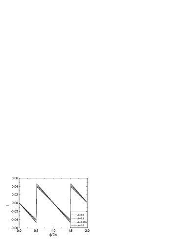
Figure 2: The persistent current in anisotropic Heisenberg spin ring versus flux for different anisotropic parameters $\Delta=0,1/2,\sqrt{3}/2,1$.

In the presence of external magnetic field, the hamiltonian changes into $H=H_{0}+h\sum{\overrightarrow{S_{z}}}$, in which $H_{0}$ is the origin hamiltonian [Eq. (1)] without the magnetic field. The magnetization $\sum{\overrightarrow{S_{z}}}=\frac{1}{2}(N-2M)$, $H=H_{0}+\frac{h}{2}(N-2M)$. For $h=0$, the ground state of this system is spin singlet(N=2M), while for $h\neq 0$, the ground state is no longer spin singlet, the magnetic field may flip some spins. For example, when $h=0.2$, the lowest energy state of the system with 42 spins is $M=20$ rather than $M=21$. In Fig. (3), we plot the dependence of the ground-state magnetization as a function of the external field.

Figure 3: The magnetization M of of the lowest energy state as a function of external magnetic field when $\Delta=0.5$.

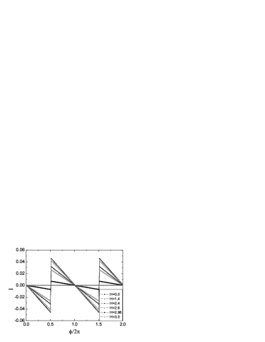
Figure 4: The persistent current as a function of the flux under the different external magnetic fields when $\Delta=0.5$.

We can then calculate the spin current. In Fig. (4), we plot the persistent current at different magnetic fields for anisotropy $\Delta=0.5$. We find that the shape of the current as a function of flux is unchanged, but the amplitude of the spin current decreases when the external magnetic field increases. And when $h$ is small the amplitude decreasing velocity is slower than it when h is much larger. After $h\geq 3.0$, the persistent current decreases to zero because all the spins are polarized by the external magnetic field.

IV the pair entanglement

We now turn to the calculation of the ground state concurrence $C$ as a function of the total magnetic flux $\phi$. Because the hamiltonian is invariant under translation, the entanglement between any two nearest neighboring sites is independent of site index. When $\Delta\neq 1$, Eq. (1) becomes q-deformed SU(2) algebra with $\Delta=(q+q^{-1})/2$. Together with the $Z^{2}$ symmetry, we have $[H,S^{z}]=0$, which simplifies the reduced density matrix $\rho_{l(l+1)}$ of two neighbor sites as

$$\rho_{l(l+1)}=\left({\begin{array}[]{*{20}c}{u^{+}}&0&0&0\\ 0&{w_{1}}&z&0\\ 0&{z^{*}}&{w_{2}}&0\\ 0&0&0&{u^{-}}\\ \end{array}}\right)$$

in the standard basis $|\uparrow\uparrow>,|\uparrow\downarrow>,|\downarrow\uparrow>$, and $|\downarrow\downarrow>$. The energy of a single pair in the system is $E/N=Tr[\rho_{l(l+1)}H_{l}]$, where $H_{l}$ is the part of the Hamiltonian between site $l$ and $l+1$, due to the translational invariance. From the definition of entanglement, we can easily find that the concurrence of anisotropic Heisenberg ring can be calculated as wang2002 :

$$C=\frac{1}{2}\max(0,|E_{gs}/N-\Delta G_{l(l+1)}^{zz}|-G_{l(l+1)}^{zz}-1),$$ (8)

where $G_{l(l+1)}^{zz}$ is the two-site correlation function defined by $G_{l(l+1)}=Tr[\exp(-\beta H)\sigma_{lz}\sigma_{l+1z}]/Z=-\frac{2}{N\beta}\frac{\partial lnZ}{\partial\Delta}$, where $\beta=1/T$, and $Z$ is the partition function. $E_{gs}$ is the ground-state energy. In order to obtain the concurrence, we calculate the correlation first. From the definition of the two-site correlation function, we know that once the $\Delta$-dependent eigenenergy $E(\Delta)$ is obtained, the correlation function is simply the first derivative of $E(\Delta)/N$ with respect to $\Delta$. Then we obtain the concurrence as a function of $\Delta$ as plotted in Fig. (5).

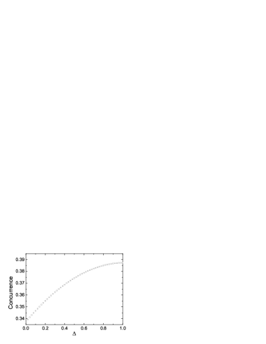
Figure 5: The concurrence of XXZ spin ring as a function of $\Delta$ for a system with 42 spins.

This result was also noticed in the Gu et al ’s work  Gu . They obtained an approximative function around the critical point $\Delta=1$ as $C_{0}-C_{1}(\Delta-1)^{2}$ where $C_{0}=2\ln 2-1\simeq 0.386$, $C_{1}=2\ln 2-\frac{1}{2}-\frac{2}{\pi}-\frac{2}{\pi^{2}}\simeq 0.047$. The largest value of concurrence at $\Delta=1$ is the result of competition between quantum fluctuation and ordering. This seems to be independent of the system size: five qubits were considered in Ref. wang , while 1280 sites were considered in Ref. Gu .

Further more, we study the influence of the magnetic flux. The concurrence as a function of the flux is plotted in Fig. (6) and in Fig. (7) for two different anisotropics $\Delta$.

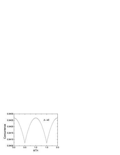
Figure 6: The concurrence as a function of flux when $\Delta\rightarrow 0$.

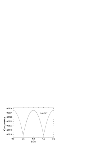
Figure 7: The concurrence as a function of flux when $\Delta\simeq 0.707$.

We find that the ground-state concurrence is also a periodic function of the flux. The locations of maximum concurrence are those of minimum energy. When the ground-state energy increases from the minimum to the maximum value, the corresponding concurrence reduces from the maximum value to the minimum. The minima of the concurrence also correspond to the energy level crossings of the ground state and the first excited state.

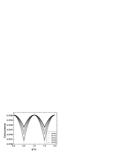
Figure 8: The concurrence as a function of flux at different magnetic fields when $\Delta=0.5$. The lines with $h\neq 0$ are shifted along $y$ axis in order to make the maximal value be the same.

In the presence of the external magnetic field, the ground state in the same fashion as Fig.(1). We calculate the ground state concurrence as a function of flux at different magnetic fields, and find that when the magnetic field increases, the value of the concurrence also increases. However, the amplitude change of the concurrence decreases as the magnetic field increases as we can see in Fig.(8), after we shift these different lines along $y$ axis so that the maximum coincide. When the spins are all fully polarized, the concurrence is independent of the flux.

V SUMMARY and discussion

In summary, we have studied the properties of the ground state persistent current and the entanglement defined by concurrence in the anisotropic Heisenberg ring pierced by a magnetic flux $\phi$. By solving the BAE numerically, we obtain the ground state energy, the persistent current, and the concurrence, which are all periodic functions of the magnetic flux. The increasing anisotropy $\Delta$ reduces the amplitude of the persistent current. The locations of minimum concurrence are those of maximum persistent current where an energy level crossing occurs. In the presence of an external magnetic field, we find that when the value of the magnetic field increased, the amplitude of the persistent current decreases. When the magnetic field is larger than a certain value ($h=3.0$ for $\Delta=0.5$, when the spins are fully polarized), the persistent current vanishes, and the concurrence is unchanged. The value of concurrence also increases as the magnetic field increased, but the amplitude change of the concurrence decreases.

VI ACKNOWLEDGEMENTS

We would like to thank Prof. X. Wan a critical reading of the manuscript, and thank Prof. X. G. Wang some useful advices. This work was supported by NSFC grant No.10225419.

References

- (1) L. P. Lvy, G. Dolan, J. Dunsmuir, and H. Bouchiat, Phys. Rev. Lett. 64, 2074 (1990).
- (2) V. Chandrasekhar, R. A. Webb, M. J. Brady, M. B. Ketchen, W. J. Gallagher, and A. Kleinsasser, Phys. Rev. Lett. 67, 3578 (1991).
- (3) D. Mailly, C. Chapelier, and A. Benoit, Phys. Rev. Lett. 70, 2020 (1993).
- (4) B. Reulet, M. Ramin, H. Bouchiat, and D. Mailly, Phys. Rev. Lett. 75, 124 (1995).
- (5) E. M. Q. Jariwala, P. Mohanty, M. B. Ketchen, and R. A. Webb, Phys. Rev. Lett. 86, 1594 (2001).
- (6) W. Rabaud, L. Saminadayar, D. Mailly, K. Hasselbach1, A. Benot, and B. Etienne, Phys. Rev. Lett. 86, 3124 (2001).
- (7) F. Schtz, M. Kollar, and P. Kopietz, Phys. Rev. Lett. 91, 017205 (2003).
- (8) Z. L. Cao, X. P. Yu, and R. S. Han, Phys. Rev. B 56, 5077 (1997).
- (9) Y. Aharonov, A. Casher, Phys. Rev. Lett. 53, 319 (1984).
- (10) F. Schtz, M. Kollar, P. Kopietz, Phys. Rev. B 69, 035313 (2004).
- (11) G. Bouzerar, D. Poilblanc, and G. Montambaux, Phys. Rev. B. 49, 8258 (1994).
- (12) C. H. Bennett, D. P. DiVincenzo, J. A. Smolin, and W. K. Wootters, Phys. Rev. A 54, 3824 (1996).
- (13) S. Hill and W. K. Wootters, Phys. Rev. Lett. 78, 5022 (1997).
- (14) W. K. Wootters, Phys. Rev. Lett. 80, 2245 (1998).
- (15) V. Coffman, J. Kundu, and W. K. Wootters, Phys. Rev. A 61, 052306 (2000).
- (16) S. Ghose, T. F. Rosenbaum, G. Aeppli and S. N. Coppersmith, Nature 425, 48 (2003).
- (17) M. C. Arnesen, S. Bose, and V. Vedral, Phys. Rev. Lett. 87, 017901 (2001).
- (18) X. Wang, Phys. Rev. A 64, 012313 (2001).
- (19) D. Gunlycke, V. M. Kendon, and V. Vedral, Phys. Rev. A 64, 042302 (2001).
- (20) G. L. Kamta and A. F. Starace, Phys. Rev. Lett. 88, 107901 (2002).
- (21) Y. Sun, Y. G. Chen, and H. Chen, Phys. Rev. A 68, 044301 (2003).
- (22) L. F. Santos, Phys. Rev. A 67, 062306 (2003).
- (23) T. J. Osborne and M. A. Nielsen, Phys. Rev. A 66, 032110 (2002).
- (24) K. M. O ’Connor and W. K. Wootters, Phys. Rev. A 63, 052302 (2001).
- (25) V. Buzek, M. Orszag, and M. Rosko, Phys. Rev. Lett. 94, 163601 (2005).
- (26) S. J. Gu, G. S. Tian, and H. Q. Lin, Phys. Rev. A 71, 052322 (2005).
- (27) C. Dunning, J. Links, and H. Q. Zhou, Phys. Rev. Lett. 94, 227002 (2005).
- (28) A. Osterloh, L. Amico, G. Falci, and R. Fazio, Nature 416, 608 (2002).
- (29) G. Vidal, J. I. Latorre, E. Rico, and A. Kitaev, Phys. Rev. Lett. 90, 227902 (2003).
- (30) J. F. Ralph, T. D. Clark, T. P. Spiller, and W. J. Munro, Phys. Rev. B 70, 144527 (2004).
- (31) P. Jordan and E. Wigner, Z. Phys. 47, 631 (1928).
- (32) Y. Q. Li and Z. S. Ma, J. Phys. Soc. Jpn. 65 1519 (1995).
- (33) H. A. Bethe, Z. Phys. 71, 205 (1931)
- (34) M. Takahashi, Thermodynamics of One-dimensional Solvable Models (Cambridge University Press, Cambridge, 1999).
- (35) X. Wang and P. Zanardi, Phys. Lett. A 301, 1 (2002).
- (36) S. J. Gu, H. Q. Lin, and Y. Q. Li, Phys. Rev. A 68, 042330 (2003).
- (37) X. G. Wang, Phys. Lett. A, 329, 439 (2004).