Nonequilibrium and Nonlinear Dynamics in Geomaterials I : The Low Strain Regime

Abstract

Members of a wide class of geomaterials are known to display complex and fascinating nonlinear and nonequilibrium dynamical behaviors over a wide range of bulk strains, down to surprisingly low values, e.g., $10^{-7}$. In this paper we investigate two sandstones, Berea and Fontainebleau, and characterize their behavior under the influence of very small external forces via carefully controlled resonant bar experiments. By reducing environmental effects due to temperature and humidity variations, we are able to systematically and reproducibly study dynamical behavior at strains as low as $10^{-9}$. Our study establishes the existence of two strain thresholds, the first, $\epsilon_{L}$, below which the material is essentially linear, and the second, $\epsilon_{M}$, below which the material is nonlinear but where quasiequilibrium thermodynamics still applies as evidenced by the success of Landau theory and a simple macroscopic description based on the Duffing oscillator. At strains above $\epsilon_{M}$ the behavior becomes truly nonequilibrium – as demonstrated by the existence of material conditioning – and Landau theory no longer applies. The main focus of this paper is the study of the region below the second threshold, but we also comment on how our work clarifies and resolves previous experimental conflicts, as well as suggest new directions of research.

PASQUALINI ET AL. Nonequilibrium and Nonlinear Dynamics in Geomaterials D. Pasqualini, EES-9, University of California, Los Alamos National Laboratory, Los Alamos, New Mexico 87545, USA. (dondy@lanl.gov)

1 Introduction

Geomaterials display very interesting nonlinear features, diverse aspects of which have been investigated over a long period of time for a recent overview see, e.g., Ostrovksy and Johnson, 2001 and references therein]. A standard technique used to study these nonlinear features is the resonant bar experiment [Clark, 1966; Jaeger and Cook, 1979; Carmichael, 1984; Bourbie et al., 1987]. In these experiments a long rod of the material under test is driven longitudinally and its amplitude and frequency response monitored. For a linear material the resonance frequency of the rod is invariant over a very wide range of dynamical strain. An example of this behavior is shown in the results from one of our experiments on Acrylic in the top panel of Figure 1: increasing the strain up to $2\cdot 10^{-6}$ leaves the resonance frequency unchanged (note that the $x$-axis shows the change in the resonance frequency, $\Delta f$, and not the resonance frequency itself.) The resonance frequency of a rod made from a nonlinear material such as Berea sandstone behaves quite differently: When a driving force is applied to the rod, the frequency either increases or decreases (the modulus either hardens or softens) depending on the precise properties of the material. This phenomenon is well-known and a theoretical description based on quasiequilibrium thermodynamics and nonlinear elasticity has existed for a long time [see e.g., Landau and Lifshitz, 1998]; we will refer to this as the classical theory of nonlinear elasticity or simply as Landau theory.

Figure 1: Resonance curves for Acrylic, Berea, and Fontainebleau at different drives. Acrylic is a linear material used as a control in the experiments. Nonlinearity is evidenced in Berea and Fontainebleau samples by the shift in the peak of the resonance curves.

Many geomaterials, such as sandstones, belong to the general class of nonlinear materials. The second and third panel in Figure 1 display resonant bar results for two representative samples, Berea and Fontainebleau. In both cases the shift in the resonance frequency is very large and the resonance frequency decreases with drive amplitude. The strength of the nonlinear response in these materials is very large, orders of magnitude more than for metals. Consequently, it is important to check whether Landau theory still applies to these materials, and, if so, over what range of strains.

It is widely believed that geomaterials behave differently than weakly nonlinear materials because of their complex internal structure. They are formed by an assembly of more or less rigid “grains” connected via a much softer “bond” network of varying porosity. The grains make up a large fraction of the volume, between 80 and 99%. Individual grains can be very pure (as in the case of Fontainebleau, $\sim 99+\%$ quartz) or made up from several different components (as in the case of Berea: 85% quartz, 8% feldspar, plus small quantities of other minerals). Most of these materials are quite porous and their behavior changes dramatically under the influence of environmental effects, such as temperature [see e.g. Sheriff, 1978] or humidity [see e.g., Gordon and Davis, 1968; O’Hara, 1985; Zinszner et al., 1997; Van den Abeele et al., 2002]. This sensitivity to the environment makes controlled studies difficult, as the experiments must be carried out in such a way that these effects are demonstrably under control.

Another difficulty in measuring the frequency response of sandstones arises from the brittleness of rocks. If the samples are driven too hard, microcracks can be induced and the resulting behavior of the material can change dramatically. In addition, driving can also induce long-lived nonequilibrium macrostates that relax back over a long period of time ($\sim$ hours). Thus, it is important to ensure – by repeating a given drive protocol on the same sample and verifying that the material response does not change from one experiment to the next – that the samples have not been altered from their original condition and the environment is unchanged over the set of observations. The experiments described in this paper were carried out in this way. Furthermore, the very low strain values ensured that sample damage rarely occurred.

One goal of this work is to clarify, using new and existing data, conflicting observations in the literature, and to present a description of the “state of the art” at low strain amplitudes. Here we restrict ourselves mainly to the question of dynamic nonlinearity and do not take up the equally important question of the nature of loss mechanisms and their connection and interaction with the nonlinear (compliant) behavior underlying the frequency shift.

In the past, several different groups have carried out resonant bar experiments. Gordon and Davis [1968] investigated a large suite of crystalline rocks, including Quartzite, Granite, and Olivine basalt, at strains between $10^{-9}<\epsilon<10^{-3}$. Their main objective was to measure the loss factor $Q^{-1}$ (or the internal friction $\phi$ in their terminology) as a function of strain and the ratio of stress and strain. In order to cover the large strain range they divided their experiments in two components: for $10^{-9}<\epsilon<10^{-5}$ they used the driven frequency method, driving the rocks at very high frequencies, and for $10^{-5}<\epsilon<10^{-3}$ they made direct measurements of the stress-strain curve. Their main findings are the following. (i) The loss factor is quite insensitive to the strain amplitude, diverging from a constant value only at high strains. At these high strains they conclude that this increase in $Q^{-1}$ is the result of internal damage. (ii) $Q^{-1}$ is highly structure sensitive, i.e., it is sensitive to the details of the microstructure of the rock. (iii) $Q^{-1}$ increases as the temperature increases. They conclude that this increase is due to grain-interface displacement, and therefore alteration of the internal structure of the rock. (iv) At large strains they find static hysteresis with end-point memory.

Following up on Gordon and Davis [1968], McKavanagh and Stacey [1974] and Brennan and Stacey [1977] performed another set of stress-strain loop measurements on granite, basalt, sandstone, and concrete. Their main objective was the measurement of stress-strain loops below strain amplitudes of $\epsilon=10^{-5}$, since Gordon and Davis [1968] had reported that $Q^{-1}$ above this limit was no longer a linear function of the applied strain. McKavanagh and Stacey [1974] were able to go down to strains of $10^{-6}$. (Note that this level is still above the strain at which we found nonequilibrium effects to be important, TenCate et al. [2004].) At these strains they found that the hysteresis loops for sandstone were always cusped at the ends. Another interesting result was that below a certain strain amplitude the shape of the loop became independent of the applied strain amplitude. From this they concluded that even at the very smallest strain amplitudes, cusps should continue to be present in stress-strain loops. (However, Brennan and Stacey [1977] noted that for granite and basalt, the stress-strain loops do become elliptical for strains lower than $10^{-6}$.) In view of our recent results [TenCate et al., 2004] this conclusion might have been drawn without having enough evidence at low enough strain amplitudes. We return to this point later in Section 4.4.

Winkler et al. [1979] conducted experiments with Massilon and Berea sandstone at strain amplitudes between 10^-8 and 10^-6. The main goal was to determine the strains at which seismic energy losses caused by grain boundary friction become important but softening of the resonance frequency with strain amplitude was also investigated. They concluded that the losses are only important at strains larger than were investigated. Additionally, they found that the two sandstones investigated displayed nonlinear features dependent on several external parameters, such as water content or confining pressure. They find that the loss factor is independent of strain below strains of $5\cdot 10^{-7}$ while at relative large strain ( $>10^{-6}$) there is a clear increase, in agreement with Gordon and Davis [1968]. The main drawback of the experiments by Winkler et al. [1979] is the relative lack of data points, especially in the very low strain regime; the quality of the repeatability of their measurements on the same sample is also not shown. In this respect, our work significantly improves on previous results; we increase the number of measurement points in the low strain regime by a factor of five in comparison to Winkler et al. [1979], allowing a more robust analysis of the data.

More recently, Guyer et al. [1999] and Smith and TenCate [2000] analyzed a set of resonant bar experiments with Berea sandstone samples also at low strains. The conclusions they reached, however, were in strong disagreement with the older results of, e.g., Winkler et al. [1979]. Instead of the expected quadratic behavior of the frequency shift with drive at very low strains – an essential prediction of Landau theory – they reported an ostensibly linear dependence, claimed to hold down to the smallest strains. We note that such a linear softening in several material samples was also reported in Johnson and Rasolofosaon [1996] (see also references therein), albeit at significantly higher strains.

This surprising behavior was claimed to be consistent with predictions of a phenomenological model originally developed to explain (static) hysteretic behavior in geomaterials at very high strains [the Preisach-Mayergoyz space (PM space) model]. In this model a rock sample is described in terms of an ensemble of mesoscale hysteretic units [McCall and Guyer, 1994; Guyer et al., 1997]. By applying the PM space model to low-strain regimes, a linear dependence of the frequency shift with drive can be obtained. By its very nature, the model also predicts the existence of cusps in low-amplitude stress-strain loops. As discussed in Section 4.4, however, we do not detect cusps in stress-strain loops at low strains.

Motivated partly by these very different findings on similar sandstones and with similar experimental set-ups, we embarked on a set of well-characterized resonant-bar experiments using Fontainebleau and Berea sandstone samples TenCate et al. [2004]. Broadly speaking, our findings for the resonance frequency shift confirm the original results of Winkler et al. [1979]; below a certain strain threshold $\epsilon_{M}$ both sandstones displayed the expected quadratic behavior. In addition, we were able to show that previous claims of a linear shift at high strains are actually an artifact due to the material conditioning mentioned above at strains higher than $\epsilon_{M}$, and that a simple macroscopic Duffing model provides an excellent mathematical description of the experimental data without going beyond Landau theory (as PM-space models explicitly do, by adding nonanalytic terms to the internal energy expansion). Thus, we established that, to the extent macro-reversibility holds, the predictions of classical theory are in fact correct.

In this paper we extend our previous analysis by adding an investigation of energy loss (via the resonator quality factor $Q$), dynamical stress-strain loops, and harmonic generation. We carry out the same experiment several times with the same sample to demonstrate environmental control and repeatability. The data analysis is based on a Gaussian process model to avoid biasing from nonoptimal fitting procedures applied to experimental data. The Duffing model introduced in our previous work is shown to be nicely consistent with the newer results. The predictions of this model for the quality factor, the frequency shift, and hysteresis cusps (null prediction) all hold within experimental error at strains below $\epsilon_{M}$. At higher strains, this simple model breaks down – as it must – due to the (deliberate) exclusion of nonequilibrium effects. Finally, we have reanalyzed a subset of the data which were taken in 1999 [Smith and TenCate, 2000] and had led to very different conclusions for Berea samples. We show that the interpretation of the data in the earlier papers was incorrect and demonstrate that the experimental data are actually in good agreement with our present findings [this paper and TenCate et al., 2004].

The paper is organized as follows. First, in Section 2 we describe the experimental set-up in some detail. Next, in Section 3 we explain how we analyze the data, especially how we determine the peaks of the resonance curves and how our procedure allows us to determine realistic error bars. In Section 4 we discuss the results from the experiments. A simple theoretical model that describes the experimental results is presented in Section 5. We confront previous findings in very similar experiments with our new results in Section 6 and conclude in Section 7.

2 Experiments

The samples used in the experiments are thin cores of Fontainebleau and Berea sandstone, 2.5 cm in diameter and 35 cm long. As established by X-ray diffraction measurements, the Fontainebleau sandstone is almost pure quartz ($>$99% with trace amounts of other materials); Berea sandstone is less pure having only 85$\pm$8% quartz with 8$\pm$1% feldspar and 5$\pm$1% kaolinite and approximately 2% other constituents. Fontainebleau sandstone has grain sizes of around 150 $\mu$ and a porosity of $\approx$ 24%. Berea sandstone samples have grain sizes which are somewhat smaller, $\approx$ 100 $\mu$, with a porosity of about 20%.

A small Bruel&Kjær 4374 accelerometer is carefully bonded to one end of each core sample with a cyanoacrylate glue (SuperGlue gel, Duro). The accelerometers are an industry standard, and are well characterized. With perfect bonding between accelerometer and rock, the accelerometer – and the associated B&K 2635 Charge Amp – has a flat frequency and phase response to 25 kHz. With poor bonds, the upper frequency limit of the flat response drops. Thus, great care is taken to establish a good bond between accelerometer and sample. Each accelerometer is first qualitatively tested (i.e., finger pressure) to be sure of a strong bond. Furthermore, before the samples are placed in the environmental isolation chamber (discussed below) for measurements, a comparison of the accelerometer response with a laser vibrometer (Polytec) is made and accelerometers are rebonded if the frequency responses differed noticeably. In any case, it is important to point out that for the samples used in this study, all of the resonance frequencies are below 3 kHz, nearly an order of magnitude below the upper frequency flat response limit for the accelerometer/charge amp combination.

The source excitation is provided by a 0.75 cm thick piezoelectric disk epoxied (Stycast 1266) to the other end of the sample core and backed with an epoxied high impedance backload (brass) to ensure that most of the acoustic energy couples into the rock sample instead of the surrounding environment. Resonances in the backload ($>~{}$50 kHz) are much higher than the frequencies and resonances of the sample and thus are not excited in our experiments.

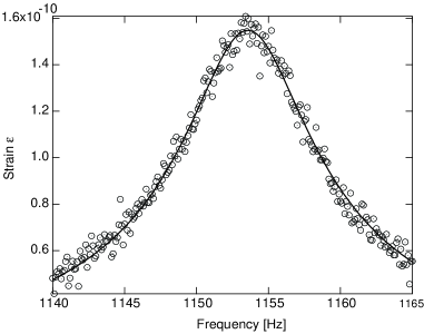
Figure 2: Low-amplitude drive resonance curve for Fontainebleau sandstone. The solid curve is a Lorentzian fit to the data points.

For all the experiments described here, the lowest order longitudinal mode (the first Pochhammer mode) is excited. (We note that the mass of the brass backload lowers the center frequencies of the Pochhammer mode resonances somewhat but does not affect the shape of a resonance curve.) Resonance curves are easy to measure and analyze and fairly high strains can be attained without requiring a high-power amplifier (with its frequently accompanying nonlinearities). For the Fontainebleau sandstone the lowest resonance frequency is around 1.1 kHz; for the Berea sandstone the lowest resonance frequency is around 2.8 kHz. Measured values for the quality factor $Q$ of these resonances are about 130 for the Fontainebleau sandstone sample and about 65 for the Berea sandstone sample. The lowest order Pochhammer mode has both compressional and shear components but the motion is nevertheless quasi-one-dimensional and the bulk of the sample participates in the wave motion associated with the resonance. As higher-order Pochhammer modes begin to resemble surface waves, only the very lowest frequency modes are examined here.

The samples are suspended at two points with loops of synthetic fiber (dental floss) or thin O-rings. Different suspension points slightly alter the lowest Pochhammer mode resonance frequencies but these differences are much smaller than differences caused by even slight changes of temperature; moreover, and perhaps more importantly, once the bar is mounted, the resonance frequencies do not change with increasing drive levels when tested with a standard (an acrylic bar). Suspended in this way (stress-free ends) the sample’s lowest Pochhammer resonance frequency corresponds to roughly a half-wavelength in the sample.

Since most rocks are extremely sensitive to temperature and temperature changes [Ide, 1937] – with relaxation times of several hours – we have built a sample chamber for effective environmental isolation. An inner 3/4-inch-wall plexiglass box with caulked seams holds both the samples which are suspended from the top of the box. Air-tight electrical feedthroughs are available for driver and accelerometer connections. The entire chamber is flushed with N₂ gas and then placed inside another (larger) plexiglass box and surrounded with fiberglass insulation and sealed. The inner sample chamber also sits on top of gel pads for vibration isolation. The complete isolation chamber is placed in a room whose temperature is controlled with a thermostat and typically varies by no more than 3 degrees C. Measured resonance frequencies of samples in this box have been stable to within 0.1 Hz.

To get the most precise measurements possible, we use an HP 3325B Frequency synthesizer with a crystal oven for frequency stability as the signal source. The signal from the HP 3325B is fed into the reference input of an EG&G 5301A Lock-In amplifier which compares that reference signal with the measured signal from the accelerometer via a B&K 2635 charge amplifier. The whole experiment, including data acquisition, is computer controlled via LabVIEW and a GPIB bus. To drive the source, the signal from the HP frequency synthesizer is fed into a Crown Studio Reference I amplifier and matched to the (purely capacitive) piezoelectric transducer via a carefully constructed and tested linear matching transformer.

To test all the electronics for linearity, we have constructed several known linear sample standards of nearly identical geometry to the rock samples. The density, sound speed, and $Q$’s of the samples are chosen such that the mechanical impedances $\rho\cdot c$ are similar to those of the rock samples. These “standard” samples are driven with identical source/backloads and at levels similar to those experienced by the rock samples. No nonlinearities have been seen; results for an acrylic rod are shown in Figure 1.

With the present isolation system, we have verified long-term frequency stability of the samples to $\pm$ 0.1 Hz (corresponding to a long-term thermal stability inside the chamber of 10 mK), which is close to how well the peak of the frequency response curve can be determined at the lowest levels of strain shown in this paper. To test the sensitivity of the Lock-In amplifier and assembled apparatus, we have measured a resonance curve on the Fontainebleau sample at an extremely low drive level. The result is shown in Figure 2. The acceleration measured by the accelerometer has been converted to strain (the open circles) using the driving frequency $f$ via $\epsilon=\ddot{u}/(4\pi Lf^{2})$ following the convention in TenCate et al. [2004]. Even though the peak strain near the resonance frequency is only about 1.6 $\cdot 10^{-10}$, the shape of the resonance curve is clear with only minimal noise obscuration: a Lorentzian curve is an extremely good fit to the data as shown by the solid line. (Error bars are not shown for clarity.) With computer control and long-term temperature stability due to the isolation chamber, this experimental setup permits long enough times to take data over a large – and an order of magnitude lower – range of strains not studied previously.

3 Data Analysis

The basic quantities measured in a resonance experiment are the frequency $f$ and the accelerometer voltage $V$, which is automatically converted into acceleration $\ddot{u}$. It is convenient to translate the acceleration to a strain variable in order to make the comparison of different samples with different lengths easier. As stated earlier, we employ the convention $\epsilon=\ddot{u}/(4\pi Lf^{2})$, where $L$ is the length of the bar. These measurements lead to resonance curves as shown e.g., in Figure 1. The task now is to determine the peaks of the resonance curves, tracking the shift of the resonance frequency as a function of the strain as displayed in Figure 3.

Figure 3: Resonance frequency shift $\Delta f$ as a function of the effective strain $\epsilon$ for the three samples shown in Figure 1.

In the past, different methods have been suggested to analyze data from low-strain resonant bar experiments [earlier attempts include Guyer et al., 1999; Smith and TenCate, 2000]. In this paper we use a statistical analysis based on a nonparametric Gaussian process to model the strain $\epsilon$ as a function of the driving frequency $f$. The flexibility of the Gaussian process model for strain allows for estimation of the resonance frequency and resulting strain $(f^{*},\epsilon^{*})$ without assuming a parametric form for the dependence of strain on driving frequency. Drawbacks of using a parametric model can include understated uncertainties regarding resonance quantities $(f^{*},\epsilon^{*})$ and excessive sensitivity to measurements far away from the actual resonance frequency. The nonparametric modeling approach avoids both of these possible pitfalls.

For a given experiment, observations $(f_{i},\epsilon_{i}),\;i=1,\ldots,n$ are taken. The observed strain is modeled as a smooth function of frequency plus white noise $\delta$:

$$\epsilon_{i}=z(f_{i})+\delta_{i},\,i=1,\ldots,n,$$ (1)

where the smooth function $z(f)$ is modeled as a Gaussian process and each $\delta_{i}$ is modeled as an independent $N(0,\sigma^{2})$ deviate. The Gaussian process model for $z(f)$ is assumed to have an unknown constant mean $\mu$ and a covariance function of the form

$$C[z(f_{i}),z(f_{j})]=\sigma^{2}_{z}\rho^{-|f_{i}-f_{j}|^{2}}.$$ (2)

The model specification is completed by specifying prior distributions for the unknown parameters $\sigma^{2}$, $\mu$, $\sigma^{2}_{z}$, and $\rho$. After shifting and scaling the data so that the $f_{i}$’s are between 0 and 1, and the $\epsilon_{i}$’s have mean 0 and variance 1, we fix $\mu$ to be 0 and assign uniform priors over the positive real line to $\sigma^{-2}$ and $\sigma^{-2}_{z}$, and a uniform prior over [0,1] to $\rho$.

The resulting analysis gives a posterior distribution for the unknown function $z(f)$ which we take to be the resonance curve. This posterior distribution quantifies the updated uncertainty about $z(f)$ given the experimental observations. We use a Markov chain Monte Carlo (MCMC) approach to sample realizations from the posterior distribution of $z(f)$ over a dense grid of points in the neighborhood of the resonance frequency $f^{*}$ [Banerjee et al., 2004]. From each of these MCMC realizations of $z(f)$ the resonance frequency $f^{*}$ and the corresponding maximum strain $\epsilon^{*}=z(f^{*})$ are recorded. This creates a posterior sample of pairs $(f^{*},\epsilon^{*})$ which are given by the dots in Figure 4(a). Figures 4(b) and 4(c) show the posterior uncertainty for $f^{*}$ and $\epsilon^{*}$ separately with histograms of these posterior samples. We use the posterior mean as point estimates for $f^{*}$ and $\epsilon^{*}$. Later in the paper we use error bars that connect the 5th and the 95th percentiles of the posterior samples to quantify the uncertainty in our estimates.

4 Experimental Results

4.1 Memory Effects and Conditioning

We have recently established the existence of two strain regimes [TenCate et al., 2004]. As mentioned earlier, in the first regime (strains below $\epsilon_{M}$) the material displays a reversible softening of the resonance frequency with strain, while in the second regime, (nonequilibrium) memory and conditioning effects become apparent. The second regime is entered at the strain threshold $\epsilon_{M}$ which depends on the material and the environment (e.g., temperature, saturation etc.). To determine $\epsilon_{M}$ for these samples, the following experiments are performed.

A reference resonance curve is obtained at the lowest strain possible. The resonance frequency is determined and used as a reference frequency $f_{0}$ for the following procedure. The source excitation level is increased, a new resonance curve is obtained, and then followed immediately by dropping the excitation level back in an attempt to repeat the reference resonance curve. If there are no memory effects, the repeated curve’s resonance frequency should match the initial reference frequency. If memory effects are at play, they will persist and the repeated curve’s peak resonance frequency will be lower than the original. An example of this is shown in Figure 5. This procedure is repeated for incrementally increasing excitation levels until memory effects become measurable. The excitation level (and strain) where memory effects first become noticeable defines $\epsilon_{M}$ for that sample.

Figure 4: (a) Resonance curve for Fontainebleau at a strain $\sim$2$\cdot 10^{-9}$. The central cluster of dots is the MCMC posterior sample of pairs (f^∗, $\epsilon^{*}$) that define the resonance peak. Frequency peak distribution (b) and frequency peak strain distribution (c) from the MCMC analysis for the same resonance curve shown in (a).

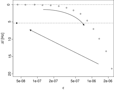
Figure 5: Example of resonance frequency shift showing the conditioning effect. The drive is increased up to a strain of $2\cdot$$10^{-6}$ and afterwards the rock is driven again at the lowest strain. The black dot shows the value of the resonance frequency peak after the last drive application. The difference between the two values for $\Delta f$ at the lowest strain demonstrates the effect of conditioning.

The existence of the two regimes delineated by $\epsilon_{M}$ is crucial to understanding and interpreting the dynamical behavior of geomaterials. Although it is possible to describe the nonlinearity of the material at strains below $\epsilon_{M}$ with classical theory [Landau and Lifshitz, 1998], above $\epsilon_{M}$ the experimental results are complicated by conditioning effects due to the nonequilibrium dynamics of the rock. Disentangling the intrinsic nonlinearity of the material and these nonequilibrium effects is very difficult and the frequency shifts in dynamical experiments at strains above $\epsilon_{M}$ do not have a simple interpretation. In particular, classical elasticity theory assumes thermodynamic reversibility and therefore cannot be applied in this essentially nonequilibrium situation. By the same token, classical theory cannot be tested by experiments carried out in this regime. As discussed in the Introduction, previous experimental data were interpretated without properly taking the existence of these different regimes into account [e.g., Guyer and Johnson, 1999]. This, along with incorrect analysis of the experimental data (see the discussion below), led to claiming evidence for nonclassical behavior where in fact none existed. Nevertheless, it is clear that a new theoretical framework for the second regime, one that combines nonlinearity with nonequilibrium dynamics, is definitely needed.

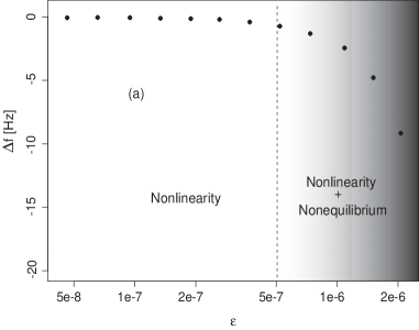
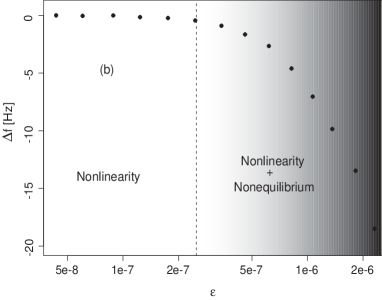
Figure 6: Resonance frequency shift versus strain. The first regime where the material displays only an intrinsic reversible nonlinearity is shown unshaded, and the second regime which combines nonlinear and nonequilibrium effects is shaded in gray. The threshold strain for Berea is $\epsilon_{M}\simeq$ 5$\cdot 10^{-7}$ (a) and for Fontainebleau is $\epsilon_{M}\simeq$ 2$\cdot 10^{-7}$ (b). Since $\epsilon_{M}$ is not only a material specific constant but can also depend on environmental variables, such as temperature and humidity, we show the regime in which nonlinearity and nonequilibrium are mixed, not as one solid block, but rather as a region in different shades of gray. It is important to note that the data points in the shaded regions depend on the (temporal) experimental protocol whereas the data points in the unshaded regions characterize an invariant behavior.

Figures 6 (a) and (b) show our data for the resonance frequency shifts versus strain for Berea and Fontainebleau samples respectively. The first regime, where the material displays only the intrinsic reversible nonlinearity is shown in the unshaded area, whereas the regime which combines nonlinear and nonequilibrium dynamical effects is shaded in gray. The strain threshold for Berea is $\epsilon_{M}\simeq$ 5$\cdot 10^{-7}$ and 2$\cdot 10^{-7}$ for Fontainebleau under the present experimental conditions. The data points in the gray region are history-dependent, and change depending on the way the experimental protocol is implemented, whereas the data points in the unshaded region are insensitive to such changes, provided one begins with the rock in an unconditioned state. For the remaining part of the paper we will focus only on the intrinsic nonlinear regime which is uncontaminated by conditioning effects and allows for a simple interpretation of the experimental data.

4.2 Intrinsic Nonlinearity

In this section we describe experimental results for strains below $\epsilon_{M}$. In this regime, the data are free from memory and conditioning effects and the samples display a reversible softening of the resonance frequency with strain. For this reason it is possible to speak of – and analyze – the intrinsic nonlinearity of the material. As discussed in some detail in the Introduction, the previous history of resonance measurements and the analysis of the associated results is somewhat confusing. On the one hand, there are claims that geomaterials display essentially nonclassical nonlinear elastic behavior down to very low strains ($10^{-8}$) [Guyer and Johnson, 1999] with no evidence for a crossover to elastic behavior. On the other hand, earlier findings [Winkler et al., 1979], albeit with generous error bars, are inconsistent with these claims.

In order to investigate this issue in a systematic and controlled fashion, we carried out repeatable resonance bar experiments at strains as low as $10^{-9}$ following the experimental protocols discussed above; these strains are an order of magnitude lower than those previously investigated.

The results for the resonance frequency shift $\Delta f$, $\Delta f=f_{0}-{\Omega}/{2\pi}$ where $\Omega$ is the (linear) resonance radian frequency, as a function of the effective strain $\epsilon$ for Fontainebleau and Berea sandstone samples are shown in Figure 7. The measured strain for Fontainebleau ranges from $2\cdot 10^{-9}$ to $\epsilon_{M}\simeq 2\cdot 10^{-7}$ and from $2\cdot 10^{-9}$ to $\epsilon_{M}\simeq 5\cdot 10^{-7}$ for Berea. We observe a resonance frequency shift of 0.45 Hz for Fontainebleau and 0.5 Hz for Berea in the regime below $\epsilon_{M}$. The error bars shown in Figure 7 are calculated using the MCMC analysis as described in Section 3. The strain error bars are smaller than the symbols used in the figures. The error bars for $\Delta f$ for Berea are larger than the ones for Fontainebleau because of the smaller $Q$ for the Berea sample: the Berea resonance curves are much wider, making the peak determination more uncertain. The solid lines in Figure 7 represent the prediction of a theoretical model with a Duffing nonlinearity described in detail in Section 5.

We find that the resonance frequency softens quadratically with increasing drive amplitude until the strain reaches $\epsilon_{M}$, beyond which value conditioning effects also enter. This behavior can be fully described by classical nonlinear theory. At very low strains, $\epsilon_{L}\sim 10^{-8}-10^{-7}$ (lower end for Fontainebleau, upper end for Berea) the samples are effectively in a linear elastic regime. At these low strains there is no discernible dependence of the resonance frequency on the strain – the materials behave linearly to better than 1 part in $10^{4}$. Our results are in qualitative agreement with previous work by Winkler [Winkler et al., 1979], but in contradiction with other results, Guyer et al. [1999]; Guyer and Johnson  [1999], and Smith and TenCate [2000]. We will study this contradiction in detail in Section 6.

4.3 Quality Factor

Energy loss in solids is mostly characterized by a frequency-independent loss factor (“solid friction”) in contrast to liquid friction. Nevertheless, rocks are known to display characteristics of liquid friction as a function of pore fluid loading [e.g., Born, 1941] with an associated dependence of the loss factor $1/Q$ ($Q$ is also termed the quality factor) on the frequency. It appears that the unusual nature of wave attenuation in geosolids remains to be fully studied and understood [Cf. Knopoff and McDonald, 1958]. As pointed out by Knopoff and McDonald, a frequency independent $Q$ cannot be explained by a linear theory of attenuation, however, it is unlikely that the nonlinearity should be associated with amplitude since even for very small strains, $Q$ remains finite.

In the present work we do not focus on the dependence of $Q$ on frequency at small strains, but investigate the dependence on strain amplitude as an alternative probe of dynamical nonlinearity for effective strains $\epsilon<\epsilon_{M}$. We measure the $Q$ from the amplitude resonance curves directly, using

$$Q=\frac{\omega_{0}}{\Gamma}[1+{\cal O}(1/Q^{2})]$$ (3)

where $\omega_{0}=2\pi f_{0}$ and $\Gamma$ is the width of the response curve measured at the points $a_{0}/\sqrt{2}$ where $a_{0}$ is the peak amplitude. This definition of $Q$ is strictly valid only for linear systems but, as will be discussed further below, at low strains the amplitude response curves are effectively those of a linear system, albeit with a peak frequency shift. At leading order, the $Q$ as defined in (3) is independent of the nature of the loss mechanism (solid or liquid friction).

The loss factor thus depends on two variables, the amplitude response peak frequency and the width $\Gamma$ of the response curve. We certainly expect it to change as a function of the strain simply because $\omega_{0}$ is a function of the strain amplitude. This is, however, a very small change, fractionally of order $10^{-4}$. Aside from this expected variation, what is of more interest is whether $\Gamma$ is also a function of the strain.

In Figure 8(a) we show measurements of the variation in the relative width $\Delta\Gamma/\Gamma_{0}$ for the Fountainebleau sample. As mentioned earlier, we restrict ourselves to the strain regime below $\epsilon_{M}$ to prevent contamination of the results by nonequilibrium effects. The width $\Gamma$ can only be measured to an accuracy of $\sim 1\%$, the error bars being obtained from MCMC analysis of the resonance curves. To this accuracy, the results of Figure 8(a) demonstrate that $\Delta\Gamma/\Gamma_{0}$ is essentially constant (except for the single highest strain point) as is the case for linear systems. This result is also consistent with the predictions of the Duffing model discussed below in Section 5.

The measurement of the relative change in quality factor is shown in Figure 8(b) and, given the smallness of the frequency peak shift, simply reflects the behavior of $\Delta\Gamma/\Gamma_{0}$. We note that except for the highest strain point, our results are in agreement with a strain-independent quality factor within the displayed errors. Our results therefore contradict Guyer et al. [1999] who found a linear dependence of $Q$ on strain amplitude (over a similar strain range as measured here). To summarize, to the extent that we have investigated the strain dependence of acoustic losses ($\epsilon<\epsilon_{M}$), no unexpected behavior has been found.

Figure 7: Resonance frequency shift $\Delta f$ as a function of the effective strain $\epsilon$ for Fontainebleau and Berea samples for $\epsilon<\epsilon_{M}$. The solid lines represent predictions of a theoretical model incorporating a Duffing nonlinearity, Eqn. (23). Two different sets of data points obtained from the same samples are shown to demonstrate the robustness of the measurements. Note the logarithmic scale on the $x$-axis.

Figure 8: Fontainebleau: (a) Variation of the width $\Gamma$ of the resonance curve peak. (b) Variation of the quality factor $Q$ with strain.

4.4 Stress-Strain Loops and Harmonic Generation

Figure 9: Acceleration versus drive amplitude for the (a) Berea and (b) Fontainebleau samples. The acceleration and the drive voltage are proportional to the strain and the stress respectively. Berea: strain amplitude $2.5\cdot 10^{-7}$ at a frequency of $2754.5$ Hz; Fontainebleau: strain amplitude $10^{-7}$ at a frequency of $1154$ Hz. Note the absence of cusps.

At very low strains and at the frequencies of interest here, one would expect the resonant bar system to be essentially a damped, driven harmonic oscillator and the hysteresis curve to be an ellipse. This is in contrast to the situation in (quasi)static hysteresis where “pointed” or “cusped” loops are observed due to sources of inelasticity that do not fit in to the simple viscoelastic model. Whether low strain loops at some point become elliptical was investigated by MacKavanagh and Stacey [1974] who came to the conclusion that this was not the case at strains $\sim 10^{-5}$ for sandstone and indeed that, “– cusped loops extend to indefinitely small strain amplitudes”. On the other hand, Brennan and Stacey [1977] found that for granite and basalt, loops became elliptical at strain values lower than $10^{-6}$. These statements were made with data taken at low frequencies, less than $0.1$ Hz, thus do not directly apply to our experiment unless the underlying sources of inelasticity continue to be relevant at high frequencies.

Experimental evidence for cusped stress-strain loops led to the theoretical description of nonequilibrium dynamics in geomaterials via PM space models which are based on static-hysteretic building blocks. In previous work, it has been argued that these models provide a correct description of the dynamics of rock even at small strains [McCall and Guyer, 1994]) and at high frequencies [Cf. Guyer et al., 1999]. Our dynamical experiments allow us to analyze stress-strain loops at very low strains in the kHz frequency range and to detect the existence of pointed or cusped loops. As evident in Figure 9 below, the loops are elliptical with no evidence for cuspy behavior. Thus, we find no evidence to support the existence of “nonlinear” dissipation mechanisms – as invoked in PM space models – at kHz frequencies. In contrast, predictions of the simple Duffing model introduced in TenCate et al. [2004] and described in detail in Section 5, are completely consistent with the data.

Our experimental results are shown in Figure 9. We plot the acceleration versus the amplitude of the drive applied to the bar for both the (a) Berea and (b) Fontainebleau samples. In the case of Fontainebleau, the strain is $1\cdot 10^{-7}$ at a frequency of $1154$ Hz while for Berea the strain is $2.5\cdot 10^{-7}$ at a frequency of $2754.5$ Hz. The acceleration and the drive amplitude are proportional to the strain and the stress respectively. The acceleration and the drive voltage are measured as functions of time and the time series is stored once steady state was attained. In Figure 9, a piece of the time series is displayed and the acceleration shifted to obtain it 180^∘ out of phase with the drive voltage. For both samples, there is no evidence for cusps in the stress-strain loops.

Another important question is whether the nonlinearity evidenced by the peak frequency shift can also be detected by searching for harmonic generation in resonant bar and wave propagation experiments. The interpretation of results from wave propagation experiments is somewhat ambiguous [Meegan et al., 1993, TenCate et al., 1996] due to experimental complications (e.g., reflective losses). However, harmonic detection in (potentially much cleaner) resonant bar experiments has been previously reported (Cf. Johnson et al. [1996]). These authors found substantial harmonic generation in rock samples – including Berea and Fontainebleau – at strains as low as $10^{-7}$.

In this paper, we present our results in a search for harmonics at strains $\epsilon<\epsilon_{M}$. Figure 10 shows spectral measurements for a linear material (acrylic) and the two rock samples. The dashed lines indicate where the first, second, and third harmonics of the fundamental are expected to appear (these are not the higher Pochhammer modes). In all three cases we observe no evidence for the existence of higher order harmonics. The two small spikes which occur in the data for Plexiglass (acrylic) and Berea are due to the residual nonlinearity of the experimental apparatus.

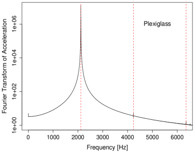
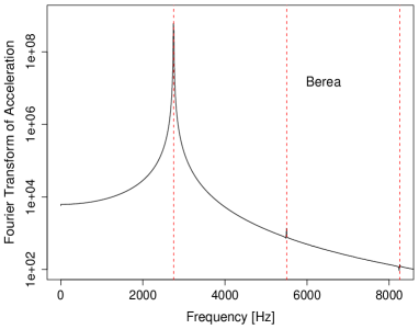
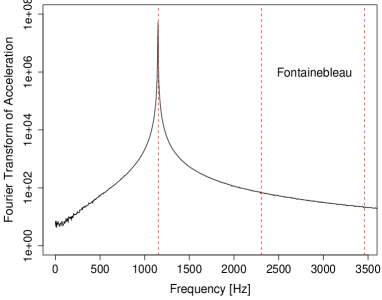
Figure 10: Fourier transform of the acceleration taken at the resonance frequency for Acrylic, Berea and Fontainebleau (semilog plot). Acrylic: nominal strain of $2.6\cdot 10^{-6}$ at frequency $2120$Hz; Berea, $2.5\cdot 10^{-7}$ at $2754.5$ Hz; Fontainebleau, $10^{-7}$ at frequency $1154$ Hz. The dashed lines show the positions of the first, second and third harmonics. Harmonic generation is not detected. The two spikes which occur in Plexiglass and Berea are due to the residual nonlinearity of the experimental apparatus.

5 The Model

In this section we introduce a simple phenomenological model which describes the nonlinear behavior of the rock samples under consideration. This model does not include a treatment of memory and nonequilibrium effects and is therefore not meant to apply in the regime where these effects become important, i.e. for strains greater than $\epsilon_{M}$. A more complex model which applies also to the higher strain regimes will be described elsewhere. As shown by us previously (TenCate et al., [2004]), a quartic (Duffing) potential nonlinearity augmenting a damped harmonic oscillator yields results that accurately describe the data in the low strain regime. This model predicts a quadratic softening of the resonance frequency as a function of drive amplitude, as expected from the theory of classical nonlinear elasticity.

The equation of motion for the displacement is taken to be:

$$\ddot{u}+\Omega^{2}u+2\mu\dot{u}+\gamma u^{3}=F\sin(\omega t),$$ (4)

where $\gamma<0$ leads to a softening nonlinearity as observed in the experiment (e.g., Figure 1). The driving force on the right hand side represents the drive applied to the rods in the experiment. The frequency $\Omega$ is the (unshifted) harmonic oscillator frequency (for $\gamma,\mu=0$) and $\mu$ is the linear damping coefficient. In the following we briefly discuss a convenient analytic approximation for the solution of Eqn. (4).

5.1 Multiscale Analysis

Since the displacement $u$ is small we can solve the equation of motion (4) analytically and predict the softening of the frequency with the drive amplitude. We employ multiscale perturbation theory to obtain a useful closed-form solution to Eqn. (4). In the following we describe how this approach works and how to extract model parameters from experimental data. [For a complete derivation of multiscale perturbation theory see Nayfeh, 1981.] While one can of course solve Eqn. (4) numerically, the analytic approach yields simple formulae which provide much better physical intuition.

A naive approach to solving Eqn. (4) would be a straightforward expansion of the displacement in the form

$$u(t,\alpha)=u_{0}(t)+\alpha u_{1}(t)+\cdots.$$ (5)

This ansatz is justified for small displacements. Inserting the expansion of $u$ in the equation of motion and keeping only terms of ${\cal O}(\alpha)$ leads to two differential equations for $u_{0}$ and $u_{1}$:

$$\ddot{u}_{0}+\Omega^{2}u_{0}=F\sin(\omega t),$$ (6)

$$\ddot{u}_{1}+\Omega^{2}u_{1}=-2\mu\dot{u}_{0}-\gamma u_{0}^{3},$$ (7)

which are simply harmonic oscillators with an inhomogeneity on the right hand side. The equation for $u_{0}$ (6) can be solved immediately and the solution inserted into the right hand side of the equation of motion for $u_{1}$ (7) specifying the inhomogeneity for $u_{1}$ completely. The solution for $u_{1}$ can now be determined and a perturbative solution for $u$ itself can be obtained by inserting $u_{0}$ and $u_{1}$ into Eqn. (5). A detailed analysis of this solution for $u(t)$ leads to the following result: for specific values of $\omega$ resonances occur, the case $\omega\sim\Omega$ leading to a primary resonance causing the solution for $u$ to diverge. To determine a solution for Eqn. (4) free from this problem, the method of multiple scales can be used [Nayfeh, 1981]. The idea is the following: besides assuming that the displacement is small, we also assume that the nonlinearity is small. In addition we assume that the excitation, the damping, and the nonlinearity are all of the same order in $\alpha$. This leads to a modified equation of motion for $u$:

$$\ddot{u}+\Omega^{2}u+2\alpha\mu\dot{u}+\alpha\gamma u^{3}=\alpha F\sin(\omega t).$$ (8)

Further we introduce two time scales, a slow scale $T_{1}=\alpha t$ and a fast time scale $T_{0}=t$ which leads to a transformation of the derivatives of the form

$$\frac{d}{dt} = D_{0}+\alpha D_{1},$$ (9)

$$\frac{d^{2}}{dt^{2}} = D_{0}^{2}+2\alpha D_{0}D_{1}+\cdots,$$ (10)

with $D_{i}=\partial/\partial T_{i}$. Expanding $u$ in the form

$$u=u_{0}(T_{0},T_{1})+\alpha u_{1}(T_{0},T_{1})$$ (11)

and keeping again only terms of order $\alpha$ leads to the following set of differential equation for $u_{0}$ and $u_{1}$:

$$D_{0}^{2}u_{0}+\Omega^{2}u_{0} = 0,$$ (12)

$$D_{0}^{2}u_{1}+\Omega^{2}u_{1} = -2D_{0}D_{1}u_{0}$$

$$-2\mu D_{0}u_{0}-\gamma u_{0}^{3}+F\sin(\omega T_{0}).$$

The difference with the previous naive expansion becomes clear immediately: While earlier the driving force was part of the differential equation for $u_{0}$, it is now part of the inhomogeneity of $u_{1}$. A general solution for $u_{0}$ is given by

$$u_{0}=A(T_{1})e^{iT_{0}}+\bar{A}(T_{1})e^{-iT_{0}}.$$ (14)

Inserting Eqn. (14) into the differential equation for $u_{1}$ (5.1) yields

$$D_{0}^{2}u_{1}+\Omega^{2}u_{1} = -(2iA^{\prime}\Omega+2i\mu A\Omega+3A^{2}\bar{A}\gamma)e^{i\Omega T_{0}}$$ (15)

$$-A^{3}\gamma e^{3i\Omega T_{0}}+\frac{1}{2}Fe^{i\omega T_{0}}+\mbox{c.c.}$$

Since we are only interested in the case $\omega\sim\Omega$, i.e., driving near to the resonance frequency we introduce a detuning parameter

$$\omega=\Omega+\alpha\sigma~{}~{}\Rightarrow~{}~{}\omega T_{0}=\Omega T_{0}+\sigma T_{1}.$$ (16)

Inserting this expression into the differential equation (15), expressing $A$ in the polar form $A=1/2a\exp{i\beta}$, defining a new parameter $\phi=\sigma T_{1}-\Omega\beta$ and $\phi^{\prime}=\sigma-\Omega\beta^{\prime}$, and eliminating the secular terms from the resulting equation, we arrive at the following solution for $u(t)$:

$$u = a\cos(\omega t-\phi)+{\cal O}(\alpha),$$ (17)

$$a^{\prime} = -a\mu+\frac{1}{2}\frac{F}{\Omega}\sin{\phi},$$ (18)

$$a\phi^{\prime} = a\sigma-\frac{3}{8}\frac{\gamma a^{3}}{\Omega}+\frac{1}{2}\frac{F}{\Omega}\cos(\phi).$$ (19)

After a sufficiently long time, $a$ and $\phi$ will reach a steady-state hence their derivatives will vanish and the left hand sides of Eqns. (18) and (19) will be zero. Squaring the equations and adding them leads to the so-called frequency-response equation

$$\Omega^{2}\mu^{2}a^{2}+a^{2}\left(\sigma\Omega-\frac{3}{8}a^{2}\gamma\right)^{2}=\frac{1}{4}F^{2}.$$ (20)

This equation can be solved with respect to $\sigma$

$$\sigma=\frac{3}{8}a^{2}\frac{\gamma}{\Omega}\pm\frac{1}{2a\Omega}\sqrt{F^{2}-4\mu^{2}a^{2}\Omega^{2}}.$$ (21)

As $\sigma$ has to be real, the maximum value for $a$ (which we label $a_{0}$) and therefore the peak of the response curve can be immediately determined:

$$F^{2}=4\mu^{2}a_{0}^{2}\Omega_{0}^{2}~{}~{}\Rightarrow~{}~{}a_{0}=\frac{F}{2\mu\Omega},$$ (22)

and therefore

$$\sigma_{0}=\frac{3F^{2}\gamma}{32\mu^{2}\Omega^{3}}.$$ (23)

Thus, the model predicts a quadratic softening of the frequency with the drive amplitude $F$. The model also predicts the invariance of the resonance curve width $\Gamma$ for any strain. Solving Eqn. (20) for $\sigma$ and substituting $a=a_{0}/\sqrt{2}$ we obtain

$$\Gamma=2\mu.$$ (24)

Note that the approximation ignores corrections of ${{\cal O}(1/Q^{2})}$. These are numerically small on the scale of the experimental errors. At this leading order of the approximation, the effect of the nonlinearity is simply to produce an effective harmonic oscillator response, with a frequency shift and peak height dependent on the drive amplitude.

5.2 Constraints on the Model Parameters from the Experimental Data

The Duffing model predicts an invariant resonance curve width $\Gamma$, therefore we first measure this quantity from the experimental resonance curves. Consistent with the above expectation, we find that $\Gamma$ is constant within $1\%$ for both samples over the applicable strain range; using relation (24) we then immediately determine the damping coefficients $\mu=27.5$ s^-1 for the Fontainebleau and $\mu=131.6$ s^-1 Berea sample, respectively. Using the definition of $\sigma_{0}=2\pi f_{0}-\Omega$ and the relation $F=2\mu\Omega L\epsilon/\pi$ we can rewrite Eqn. (23) in terms of the effective strain $\epsilon$ and the resonance frequency $f_{0}$ as:

$$f_{0}=\frac{3L^{2}\gamma}{16\pi^{3}\Omega}\epsilon^{2}+\frac{\Omega}{2\pi}.$$ (25)

The linear resonance frequency $\Omega$ and the nonlinearity parameter $\gamma$ now follow by fitting the experimental data for $f_{0}$ as a function of the effective strain using the previous equation. We obtain the following values: the nonlinearity parameter, $\gamma=-7.6\cdot 10^{19}$ m^-2s^-2 for the Fontainebleau sample, and $\gamma=-5.3\cdot 10^{19}$ m^-2s^-2 for the Berea sample, whereas the corresponding linear resonance frequencies are $7262.8$ rad/s and $17375.7$ rad/s.

5.3 Comparison of the Experimental Results with the Model

After determining model parameters as above, we compare the Duffing model predictions with the experimental results described in Section 4.

We begin by investigating the predictions for the resonance curves themselves, as given in Eqn. (20). In Figure 11 we show the results from the experiments as circles and the results from the Duffing model as solid lines for (a) Fontainebleau and (b) Berea, where (c) shows a single Berea resonance curve on a smaller range in $\Delta f$ to demonstrate more clearly how well the model works. In addition, it was shown earlier (Figure 7) how the resonance frequency shifts as a function of strain for Fontainebleau and Berea from both the experiment and the model. Figure 7 and Figure 11 clearly demonstrate the excellent agreement between the experimental data and the model predictions.

In Figure 12 we show the stress-strain loop obtained from the Duffing model: no cusps are present in agreement with the experimental results. Moreover our model indicates that the response of the bar to the external drive is dominated by the fundamental mode and there is no excitation due to mode-coupling of any higher harmonics as shown in Figure 13. This prediction is in contradiction with previous work [Johnson et al., 1996] where it was claimed that the absence of frequency softening is not sufficient to rule out nonlinearity in rocks as harmonic generation may exist even in the absence of a discernible frequency shift. Our model predictions are again in very good agreement with the experimental results.

Figure 11: Average strain amplitude $\epsilon$ as a function of drive frequency for Fontainebleau (a) and Berea (b) and (c). The reference center frequency is 1155.98 Hz for Fontainebleau and 2765.179 Hz for Berea. The open circles are the experimental data; the filled circles mark the peak positions. The solid lines are theoretical predictions from Eqn. (20). Figure (c) shows in detail the resonance curve at the highest strain for Berea.

Figure 12: Hysteresis loop as predicted by the Duffing model using Berea parameters, strain $2.7\cdot 10^{-7}$, frequency = 2765.3 Hz.

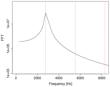
Figure 13: Spectral response from the Duffing model using Berea parameters, strain $2.7\cdot 10^{-7}$, frequency = 2765.3 Hz.

6 Comparison with Previous Results

As already discussed in the Introduction, experiments similar to the one described in this paper have been carried out in the past with somewhat confusing results. Some of them, e.g., those of Winkler et al. [1979], are in qualitative agreement with our findings though with less control over errors, while other papers claim quite different results. Among this second set of papers, two papers are experimentally very close to the present work (two of the authors of the current paper were involved in these experiments): the papers by Guyer et al. [1999] (referred to as GTJ below) and Smith and TenCate [2000] (referred to as S&T below). We now address the question why such differing conclusions were arrived at earlier: was it the experimental data themselves or were they analyzed and interpreted incorrectly? In order to provide the answer we reanalyze a subset of the older data sets investigated in GTJ and S&T.

The experiment underlying the two papers was carried out over a long span of time. The data set analyzed in GTJ is in fact a small subset of the data investigated in S&T, as stated in the second paper explictly. The sample under consideration was a Berea sandstone rod, 35 cm long and 2.4 cm in diameter (the numbers quoted in GTJ are slightly different: 30 cm length and 6 cm diameter, we verified that S&T were correct), therefore very similar to the sample used in this paper. In order to reduce effects from moisture contained in the sandstone the sample was kept under vacuum for an extended period. This increased the quality factor of the rod to $Q\sim 300$ making the analysis of the experiment easier, since the resonance curves are less broad than for lower $Q$. (In GTJ the quality factor is incorrectly quoted to be $Q=170$, the discrepancy arising due to measuring $Q$ from the width of the resonance curve at half-maximum of the amplitude rather than at $1/\sqrt{2}$ of the maximum.) The quality factor in the old experiment was therefore roughly five times higher than in the current one. The resonance frequency in the old experiment was $f\sim 2880$ Hz, which is close the resonance frequency of the sample we investigated, $f\sim 2755$ Hz. In the old experiments, different measurements were made at different temperatures, ranging from 35^∘C to 65^∘C, but for each separate measurement the temperature was controlled to approximately 0.1^∘C. The experiments were carried out in three different strain ranges: at very low strain, at medium strain, and at high strain. We will be more specific about the strain ranges below. The main result found by GTJ was a linear fall-off of the resonance frequency peak with increasing strain while S&T concluded from the same experimental data that the resonance frequency peak fell off first linearly and then quadratically with increasing strain.

Before we turn to discuss the analysis strategies followed in GTJ and S&T we first investigate a subset of the old data set in exactly the same way as in the new experiments. The results are shown in Figure 14. We randomly chose one data set taken at a constant temperature of 35^∘C. Figure 14(a) shows three sets of resonance curves at different strain ranges. The peaks of the resonance curves are determined with our MCMC analysis method as described in Section 3 and marked by the filled circles. In Figure 14(b) the peaks of the resonance curves are plotted versus the strain. From this figure the strain ranges can be read off: the low strain regime ranges from 3.1$\cdot$10^-8 to 5.8$\cdot 10^{-7}$, the medium strain regime from 1.64$\cdot 10^{-7}$ to 1.3$\cdot 10^{-6}$, and the high strain regime from 8.1$\cdot 10^{-7}$ to 2.5$\cdot 10^{-6}$. The solid lines in the low and medium strain regime represent the predictions from our model. In these two regimes the predictions from the Duffing model are excellent, and no unexpected behavior, such as a linear fall-off is observed. Note, that the model in this case works even at higher strains than the threshold found in the new experiment, although of course $\epsilon_{M}$ in the old experimental samples could have been different. The measurements in the high strain regime are contaminated by nonequilibrium effects and therefore our simple model is not applicable. To reiterate: the old data set reanalyzed by us is in complete agreement with the results from our new experiments. A threshold where the Berea sample behaves as a linear material exists, for low strains the sample behaves like a classical nonlinear material, and at very high strain, due to nonequilibrium effects, the interpretation of the data becomes very involved and does not allow for deciding between classical or nonclassical behavior.

After verifying that the old experimental data in no way contradict the results from our new experiments we now turn to the analysis strategies used in GTJ and S&T and the interpretations of their findings.

In contrast to our analysis, in which we determine the peak of every single resonant curve, GTJ analyze the data at constant strain. While this method should work in general, it has several shortcomings. First, the resonance curves analyzed in GTJ were only sparsely sampled with data points. In order to carry out the constant strain analysis, the resonance curves had to be interpolated to obtain the values at one constant strain. This fitting procedure might lead to a bias in the results with respect to the functional form of the fit applied. Second, the number of data points available for the application of the constant strain analysis decreases rapidly with strain amplitude. Third, the constant strain analysis leads to correlated error bars. (Our MCMC-based method is free from these problems.)

The results for the dependence of the resonance frequency versus strain are shown in Figure 3(a) in GTJ. The strain range shown on the $x$-axis in this plot is $10^{-8}$ to 5$\cdot 10^{-7}$ as explained in the text. The three different curves GTJ show are from different measurements and in all cases the dynamic range is very small. Consider now the lowest – and longest – of these curves, the strain range here is only 10^-7 to $3\cdot 10^{-7}$. A linear fit for this data set might naively appear to be justified, even though the data points at the higher strains are already falling off a linear fit.

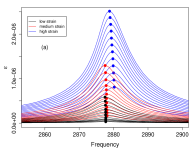
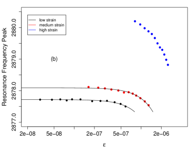
Figure 14: Comparison with previous experiments on Berea: (a) resonance frequency curves for three sets of experiments at three different strain ranges. (b) The corresponding resonance frequency peaks. Note the logarithmic scale on the $x$-axis. The solid lines represent predictions of the theoretical model, see Eqn. (23).

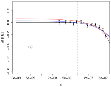
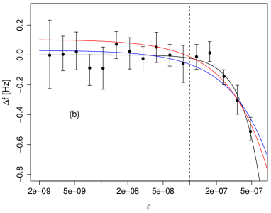
Figure 15: Comparison of different fits for (a) the old Berea data set and (b) the new Berea data set. Note the logarithmic scale on the $x$-axis. The black line shows the quadratic fit obtained from the Duffing model, the red line shows the best linear fit including data points only to the right of the dashed line. Inclusion of all data points for the linear fit makes the fit much worse.

To emphasize the importance of having sufficient dynamic range, we return to Figure 14(b) and consider only the lowest strain measurement data set, shown in detail in Figure 15(a). The dashed line marks the strain corresponding to the lowest strain in GTJ in their longest strain range measurement. We show in red the best linear fit to all the data points on the right of this line. The highest strain in GTJ was $3\cdot 10^{-7}$ so would only include 4 of the data points in Figure 15(a). If we only concentrate on the strain regime to the right of the dashed line, both fits, linear and quadratic are acceptable. But if we consider all the available data points down to the lowest strain, the linear fit fails by being too high. Therefore, in order to make a definite statement about the best fit to the data it is clearly important to have a sufficient range in strain.

It is not possible to obtain uncontaminated measurements at higher strains as discussed in detail earlier, hence extension of dynamic range requires measurements at low strains, as carried out in the present work. We demonstrate the usefulness of this in Figure 15(b) where we show once again the new Berea measurements with the quadratic fit shown in black, and the best linear fit – again only for the data points on the right side of the dashed line – in red. Inclusion of more points for the linear fit again makes the agreement much worse. It is apparent that without sufficient dynamic range it is easy to be misled in fitting a linear curve to the data. Including all the data points down to a strain of 10^-9 demonstrates the correctness of the quadratic fit. To summarize: the experimental data in GTJ is apparently correct, but the dynamic range of the data points analyzed is not sufficient to draw any conclusion regarding the nonlinear behavior of the material.

Finally we are unable to understand the remark in GTJ that the traditional theory of nonlinear elasticity predicts a value of $\Delta f/f_{0}\sim 10^{-10}$ at a strain of roughly $3\cdot 10^{-7}$. All that traditional theory predicts is a quadratic frequency shift which we do observe; the magnitude is set by a certain dynamic nonlinearity coefficient which, in effect, is measured in the experiment. No contradiction with classical nonlinear theory is observed in our experiment or indeed in the data of GTJ.

Next, we turn to the results found in S&T. One of the main objectives in that work was to investigate the dependence of the frequency shift (hence, the shift in the Young’s modulus) as a function of temperature changes. The idea was that static hysteresis mechanisms (if present at very low strains) could be due to thermal activation instead of mechanical stick-slip processes as in quasi-static experiments at much higher strain. (However, the authors did not directly investigate if the system showed cuspy hysteretic behavior in the first place.)

Experiments at temperatures ranging from 35^∘ to 65^∘ were carried out. In addition different strain regimes were investigated at different times, as shown in the previous Figure 14(a). The condition of the rock might have changed in between these different times, which could have led to a contamination of the results. Data-fitting was carried out by fitting to a simple pole response characteristic, however, the possible systematic errors in this procedure were not discussed. In addition, for each temperature, the three different sets of measurements at low, medium, and high strain were shifted in order to obtain a single measurement over a wide strain range. This approach is likely to lead to a bias in the result since the rock might have been in different metastable conditioned states for each data set.

In the final step, the relative shift in the Young’s modulus was determined and fitted by a single function for all resonance frequency shift curves, independent of the temperature at which they were taken or the resonance frequency $\omega_{0}$ (recall the different strain ranges of the data shown in Figure 14). The result of this analysis is shown in Figure 6 of S&T. It is immediately clear that a single fit to all the curves is rather dangerous and the single fit (solid line in Figure 6) does not work particularly well. The functional form of the fit – first linear and then quadratic – is therefore also not very meaningful, since no error bars are shown, any other functional form, such as pure quadratic, would have probably worked as well.

The authors’ contention that the temperature-insensitivity of the coefficients determining the frequency shift is directly related to the underlying loss mechanism – and hence rules out thermal activation mechanisms – is incorrect. The relationship between the frequency shift and the loss mechanism is yet to be elucidated: as shown in the present work for example, nonlinear frequency shifts and linear losses can easily coexist and it is well-known that the loss factor is temperature-dependent.

In summary, the measurements used in GTJ and S&T are in fact in very good agreement with our current measurements and understanding of the nonlinearities in rocks below a certain strain threshold – it is the interpretation of the data in these two papers that must be corrected. In GTJ the strain range over which the analysis was carried out was insufficient to reach any conclusive result about the fall-off of the resonance frequency peak with strain. In S&T the fitting procedure applied to the data sets seems to have led to erroneous conclusions about the behavior of $\Delta f$ versus strain.

7 Summary and Outlook

In this paper we have described a set of resonant bar experiments carried out for Berea, Fontainebleau, and Acrylic (as a linear control material) in order to investigate the dynamic compliance and loss mechanisms at low strains, between $5\cdot 10^{-8}$ and $2\cdot 10^{-6}$. To ensure isolation from environmental influences, such as temperature and humidity, an isolation chamber was employed to obtain controlled and repeatable results.

The main conclusion of our work is the demarcation of two strain regimes: in the first regime the material displays reversible softening of the resonance frequency, while in the second regime, which occurs after a material and environment-dependent threshold $\epsilon_{M}$, nonequilibrium and conditioning effects become important. Some of these results were previously reported in a short communication [TenCate et al. 2004]. Here we report the results of a detailed study for the first strain regime – below $\epsilon_{M}$ – for both Berea and Fontainebleau samples measuring quantities such as the quality factor, stress-strain loops, and amplitudes of higher harmonics. By repeating measurements on the same samples we have demonstrated the robustness of the results. At strains characteristic of reversible nonlinear behavior, the quality factor is essentially constant, but it is possible that it reduces at higher strain values. It is not unreasonable to speculate that – unlike the resonance frequency shift – the amplitude dependence of the quality factor is connected to the onset of nonequilibrium behavior, but this aspect requires further investigation.

The data analysis was carried using a statistical method based on a Gaussian process model. This parameter-free method avoids any biasing of the analysis due to fitting of the resonance curves with specific functional forms. It also determines reliable error bars for the resonance frequency shift $\Delta f$ as a function of the applied drive strength. The vast majority of previous papers analyzing similar experiments do not provide a detailed error analysis.

A theoretical framework for the experimental results is provided by a simple damped Duffing model for which closed-form results can be obtained. The Duffing model predictions are in excellent agreement with the entire set of experimental measurements over the strain regime $\epsilon<\epsilon_{M}$.

Our results are in disagreement with some of the previous work carried out with the resonant bar technique as has been pointed out at the relevant places in the main body of the paper. In two cases – Smith and TenCate, [2000] and Guyer et al., [1999] – we have reanalyzed a subset of the older experimental data and have demonstrated that the disagreement is not due to fundamental differences in the data but due to mistakes in the theoretical interpretation and analysis in these papers. Thus, one goal of this paper is simply to clarify the present state of knowledge in the low-strain regime.

While in this paper, we have focused on the reversible nonlinear regime ($\epsilon<\epsilon_{M}$), future work will target the understanding of the nonequilibrium behavior of geomaterials. The investigation of this second regime is at the same time fascinating and very challenging. It is difficult, but essential, to disentangle conditioning/nonequilibrium and nonlinear effects. New experimental strategies have to be developed for this endeavor. At the same time a theoretical framework which encompasses and explains all known physical effects needs to be developed.

- [1] Meegan, G.D., Johnson, P.A., Guyer, R.A., and McCall, K.R. (1993), Observations of nonlinear elastic wave behavior in sandstone, J. Acoust. Soc. Am., 94, 3387.
- [] McKavanagh, B. and Stacey, F.D. (1974), Mechanical Hysteresis in Rocks at Low Strain Amplitudes and Seismic Frequencies, Physics of the Earth and Planetary Interiors, 8, 246–250.
- [] Nayfeh, A.H. (1981), Introduction to Perturbation Techniques (Wiley, New York).
- [] O’Hara, S.G. (1985), Influence of pressure, temperature, and pore fluid on the frequency-dependent attenuation of elastic waves in Berea sandstone, Phys. Rev. A, 32, 472–488.
- [] Ostrovsky, L.A. and Johnson, P.A. (2001), Dynamic Nonlinear Elasticity in Geomaterials, Nuovo Cimento, 24, 1–46.
- [] Sheriff, R.E. (1973) Encyclopedic Dictionary of Exploration Geophysics (Tulsa, Okla., Society of Exploration Geophysicists).
- [] Smith, E. and TenCate, J. (2000), Sensitive determination of the nonlinear properties of Berea sandstone at low strains, Geophys. Res. Lett.,27, 1985–1988.
- [] TenCate, J.A., Van den Abeele, K.E.A., Shankland, T.J., and Johnson, P.A. (1996), Laboratory Study of Linear and Nonlinear Elastic Pulse Propagation in Sandstone, J. Acoust. Soc. Am., 100, 1383-1391.
- [] TenCate, J.A., Pasqualini, D., Habib, S., Heitmann, K., Higdon, D., and Johnson, P.A. (2004), Nonlinear and Nonequilibrium Dynamics in Geomaterials, Phys. Rev. Lett., 93, 065501–1–065501–4.
- [] Van den Abeele, K.E.A., Carmeliet, J., Johnson, P.A., and Zinszner, B. (2002), Influence of Water on the Nonlinear Elastic Mesoscopic Response in Earth Materials and the Implications to the mechanism of Nonlinearity, J. of Geophys. Res. 107, ECV4-1-11.
- [] Winkler, K., Nur, A. and Gladwin, M. (1979), Friction and seismic attenuation in rocks, Nature, 277, 528–531.
- [] Zinszner, B., Johnson, P.A., Rasolofosaon, P.N.J. (1997), Influence of change in physical state on elastic nonlinear response in rock: significance of effective pressure and water saturation J. of Geophys. Res. 102, 8105–8120.