Pomeranchuk and Topological Fermi Surface Instabilities from Central Interactions

Abstract

We address at the mean field level the emergence of a Pomeranchuk instability in a uniform Fermi liquid with central particle-particle interactions. We find that Pomeranchuk instabilities with all symmetries except $l=1$ can take place if the interaction is repulsive and has a finite range $r_{0}$ of the order of the inter-particle distance. We demonstrate this by solving the mean field equations analytically for an explicit model interaction, as well as numerical results for more realistic potentials. We find in addition to the Pomeranchuk instability other, subtler phase transitions in which the Fermi surface changes topology without rotational symmetry-breaking. We argue that such interaction-driven topological transitions may be as generic to such systems as the Pomeranchuk instability.

I Introduction

Experimental evidence of “hidden” phases of itinerant electron systems tallon_99 ; kim_03 ; grigera_04 and the prospect of realizing novel conditions in layered heterostructures and ultra-cold gases have led to increased efforts to identify unconventional phase transitions and predict their manifestations. To give three examples: the Fulde-Ferrell-Larkin-Ovchinnikov state has been proposed in organic superconductors balicas_01 , superconductor-ferromagnet heterostructures annett_05 and in imbalanced mixtures of ultracold atoms FFLO_in_atoms ; FFLO_in_atoms-2 ; a supersolid phase is a possibility in Bose gases loaded on optical lattices goral_02 ; and a “$d$-density wave” may be realized in ladder compounds DDW-2 ; DDW-3 and possibly “hide” in the phase diagram of cuprate superconductors DDW , where other hidden order parameters have been proposed varma1 ; varma2 .

In this context there has been a surge of interest in the Pomeranchuk Instability (PI) pomeranchuk_58 . Through it a Fermi liquid may enter a “nematic” state characterized by a deformed Fermi surface. It has been argued that such an instability may take place in quantum Hall systems QH ; QH-2 and in the metamagnets Sr₃Ru₂O₇ grigera_04 and URu₂Si₂ 2005-Varma-Zhu . Moreover there is evidence that the Hubbard model has a phase with a distorted Fermi surface HM ; HM-2 ; HM-3 ; HM-4 ; HM-5 ; HM-6 and the Emery model of a CuO₂ plane has been shown to have a nematic ground state in the strong coupling limit 2004-Kivelson-Fradkin-Geballe .

More generally the PI is an interesting candidate unconventional phase transition on account of its subtlety. Thus, considerable effort is going into characterizing it theoretically phase_diagram ; phase_diagram-2 ; phase_diagram-3 ; collective ; collective-2 ; collective-3 ; collective-4 ; collective-5 on the basis of phenomenological models featuring anisotropic effective interactions. This approach is proving very successful in establishing some generic features of the phase diagram phase_diagram ; phase_diagram-2 ; phase_diagram-3 and describing collective excitations and quantum critical fluctuations collective ; collective-2 ; collective-3 ; collective-4 ; collective-5 . On the other hand it sidelines the question of how the anisotropy emerges in the first place collective and what other varma_05 , perhaps even subtler instabilities may generically arise in such contexts. It is these questions that we address here.

In this paper we present a mean field (MF) theory of the PI in a three-dimensional, uniform fermion liquid with a central effective interaction potential $V(r)$. The authors of Ref. collective, have pointed out that such interaction may lead to a PI. Here we show that the emergence of the anisotropic state from a Galilean invariant fluid requires repulsion with an intermediate range of the order of the inter-particle distance. This is confirmed by explicit calculation for a model interaction potential for which the theory can be solved analytically. However we also find that the intermediate-range repulsion leads, quite generally, to a different instability in which there is no symmetry breaking but the topology of the Fermi surface changes. We discuss the nature of this subtler quantum phase transition. A few instances of the two distinct types of Fermi surface shape instabilities that we find are pictured in Fig. 1. These two types of instability compete and we show that this conclusion is robust when we consider more more realistic finite range interactions.

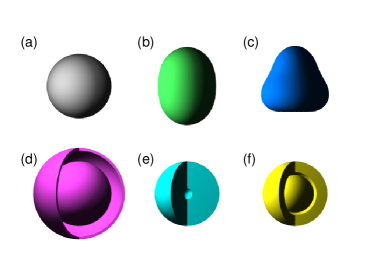
Figure 1: (color online) Different shapes and topologies of the Fermi surface. From left to right, in the first row: (a) unpolarized, undeformed Fermi sphere; (b) Fermi surface with an $l=2$ Pomeranchuk deformation; (c) $l=3$. In the second row: (d) Fermi sphere surrounded by an additional sheet of occupied states; (e) with a “hole” of vacated states at the center; and (f) with a shell of vacated states.

II Mean field theory

To motivate a microscopic theory of the PI we start by recalling the original, phenomenological theory due to Pomeranchuk pomeranchuk_58 . Like him, we start with an unpolarized Fermi sphere and consider an infinitesimal change of the occupation numbers, $N_{\mathbf{k},\sigma\sigma}\to N_{\mathbf{k},\sigma\sigma}+\delta N_{\mathbf{k},\sigma\sigma},$ arising from an angle-dependent modulation of the Fermi vector, $k_{F}\to k_{F}+\delta k_{F}\left(\theta\right)$, $k_{F}\to k_{F}+\sigma\delta k_{F}\left(\theta\right)$ in the symmetric or antisymmetric spin channel, respectively . We then use Landau’s expression for the corresponding change in the ground state energy: $E\to E+\delta E,$ with

$$\delta E = \sum_{\mathbf{k}}\varepsilon\left(\mathbf{k}\right)\delta N_{\mathbf{k}}$$

$$+\frac{1}{2}\sum_{\mathbf{k},\mathbf{k}^{\prime}}\left\{f^{s}\left(\mathbf{k},\mathbf{k}^{\prime}\right)\delta N_{\mathbf{k}}\delta N_{\mathbf{k}^{\prime}}+f^{a}\left(\mathbf{k},\mathbf{k}^{\prime}\right)\delta\mathbf{S}_{\mathbf{k}}\cdot\delta\mathbf{S}_{\mathbf{k}^{\prime}}\right\}.$$

Here $\delta N_{\mathbf{k}}=\sum_{\sigma}\delta N_{\mathbf{k},\sigma\sigma}$ and $\delta S_{\mathbf{k}}^{i}=\frac{1}{2}\sum_{\sigma,\gamma}\sigma_{\sigma\gamma}^{i}\delta N_{\mathbf{k},\gamma\sigma}.$ Requiring $\delta E<0$ leads to the PI conditions

$$1+F_{l}^{a,s}/\left(2l+1\right)<0,$$ (2)

in terms of the Landau parameters, defined by

$$f^{s,a}\left(k_{F}\hat{\mathbf{k}},k_{F}\hat{\mathbf{k}}^{\prime}\right)=\frac{\pi^{2}\hbar v_{F}}{\Omega k_{F}^{2}}\sum_{l=0}^{\infty}F_{l}^{s,a}P_{l}\left(\hat{\mathbf{k}}.\hat{\mathbf{k}}^{\prime}\right),$$ (3)

where $k_{F}$ is the radius of the Fermi sphere, $v_{F}$ is the Fermi velocity and $P_{l}\left(x\right)$ is the $l^{{\rm th}}$ Legendre polynomial. For $l=0,$ Eq. (2) describes a quantum gas-liquid transition (in the symmetric spin channel, $s$) or a Stoner instability (in the antisymmetric channel, $a$). For $l>0$ it describes a Pomeranchuk instability.

One crucial aspect of Pomeranchuk’s theory is that it describes the instability in terms of the phenomenological Landau parameters, $F_{l}^{s,a}$. Here we want to establish the mechanism whereby the PI could take place in a system with a given microscopic Hamiltonian of the form

$$H = \int d^{3}\mathbf{r}\sum_{\sigma}\hat{c}_{\mathbf{r},\sigma}^{+}\left[\frac{1}{2m}\left(\frac{\hbar}{i}\nabla\right)^{2}-\mu\right]\hat{c}_{\mathbf{r},\sigma}$$

$$+\frac{1}{2}\sum_{\sigma,\sigma^{\prime}}\int d^{3}\mathbf{r}\int d^{3}\mathbf{r}^{\prime}\hat{c}_{\mathbf{r},\sigma}^{+}\hat{c}_{\mathbf{r}^{\prime},\sigma^{\prime}}^{+}V\left(\left|\mathbf{r}-\mathbf{r}^{\prime}\right|\right)\hat{c}_{\mathbf{r}^{\prime},\sigma^{\prime}}\hat{c}_{\mathbf{r},\sigma},$$

where $V\left(\left|\mathbf{r}-\mathbf{r}^{\prime}\right|\right)$ is a local, non-retarded, spin-independent and central interaction potential. We address this question using MF theory. Our MF Hamiltonian is

$$H_{0}=\sum_{\mathbf{k},\sigma}\varepsilon_{\sigma}\left(\mathbf{k}\right)\hat{c}_{\mathbf{k},\sigma}^{\dagger}\hat{c}_{\mathbf{k},\sigma},$$ (5)

where $\hat{c}_{\mathbf{k},\sigma}^{+}\equiv\Omega^{-1/2}\int d^{D}\mathbf{r}e^{-i\mathbf{k}.\mathbf{r}}\hat{c}_{\mathbf{r},\sigma}^{+}.$ This describes independent electrons with an arbitrary dispersion relation $\varepsilon_{\sigma}\left(\mathbf{k}\right),$ which we treat as our variational parameter. Note that this MF couples only to the occupation number in $\mathbf{k}$-space, $\hat{N}_{\mathbf{k},\sigma\sigma}=\hat{c}_{\mathbf{k},\sigma}^{\dagger}\hat{c}_{\mathbf{k},\sigma}$. Our theory thus preserves translational and gauge symmetry, but it can nevertheless break rotational symmetry if the dispersion relation becomes anisotropic. For example, a nematic Fermi liquid state may be entered through a PI. It is an example of an “electronic liquid crystal state” liquid_crystal .

Although our main results refer to the ground state, the derivation of the basic equations of the theory is much simpler at finite temperature. We thus approximate the free energy by $F\approx\left\langle H-H_{0}\right\rangle_{0}+F_{0}$, where $\left\langle\ldots\right\rangle_{0}=Z_{0}^{-1}{\rm Tr}\left\{e^{-\beta H_{0}}\ldots\right\}$ with $Z_{0}={\rm Tr}\left\{e^{-\beta H_{0}}\right\}$ and $F_{0}=-\beta^{-1}\ln Z_{0}$. It takes the form

$$F = \sum_{\mathbf{k},\sigma}\left\{\begin{array}[]{c}\\ \\ \\ \end{array}\right.N_{\mathbf{k},\sigma}\left[\begin{array}[]{c}\\ \\ \end{array}\right.-\frac{1}{2\Omega}\sum_{\mathbf{k}^{\prime}}V\left(\left|\mathbf{k}-\mathbf{k}^{\prime}\right|\right)N_{\mathbf{k}^{\prime},\sigma}$$ (18)

$$+\frac{\bar{V}}{2\Omega}\sum_{\mathbf{k}^{\prime},\sigma^{\prime}}N_{\mathbf{k}^{\prime},\sigma^{\prime}}+\frac{\hbar^{2}\left|\mathbf{k}\right|^{2}}{2m}-\mu-\varepsilon_{\sigma}\left(\mathbf{k}\right)\left.\begin{array}[]{c}\\ \\ \end{array}\right]$$

$$-\frac{1}{\beta}\ln\left[1+e^{-\beta\varepsilon_{\sigma}\left(\mathbf{k}\right)}\right]\left.\begin{array}[]{c}\\ \\ \\ \end{array}\right\}$$

where $\bar{V}=\int d^{3}\mathbf{R}V\left(\left|\mathbf{R}\right|\right)$ is the uniform component of the interaction potential and $V\left(\mathbf{K}\right)=\int d^{3}\mathbf{R}e^{-i\mathbf{K}.\mathbf{R}}V\left(\left|\mathbf{R}\right|\right)$ its Fourier transform. The occupation numbers in $\mathbf{k}$-space are given by

$$N_{\mathbf{k},s}=\left[1+e^{\beta\varepsilon_{\sigma}\left(\mathbf{k}\right)}\right]^{-1}.$$ (19)

Requiring that $F$ be stationary yields

$$\varepsilon_{\sigma}\left(\mathbf{k}\right)=\frac{\hbar^{2}\left|\mathbf{k}\right|^{2}}{2m}-\mu+\frac{1}{\Omega}\sum_{\mathbf{k}^{\prime}\sigma^{\prime}}\left\{\bar{V}-\delta_{\sigma,\sigma^{\prime}}V\left(\left|\mathbf{k}-\mathbf{k}^{\prime}\right|\right)\right\}N_{\mathbf{k}^{\prime},\sigma^{\prime}}.$$ (20)

In the low-temperature limit, $\beta\to\infty,$ Eqs. (18,19) become

$$E = \sum_{\mathbf{k},\sigma}N_{\mathbf{k},\sigma}\left[\begin{array}[]{c}\\ \\ \end{array}\right.-\frac{1}{2\Omega}\sum_{\mathbf{k}^{\prime}}V\left(\left|\mathbf{k}-\mathbf{k}^{\prime}\right|\right)N_{\mathbf{k}^{\prime},\sigma}$$ (26)

$$+\frac{\bar{V}}{2\Omega}\sum_{\mathbf{k}^{\prime},\sigma^{\prime}}N_{\mathbf{k}^{\prime},\sigma^{\prime}}+\frac{\hbar^{2}\left|\mathbf{k}\right|^{2}}{2m}-\mu\left.\begin{array}[]{c}\\ \\ \end{array}\right];$$

$$N_{\mathbf{k},\sigma} = \Theta\left[-\varepsilon_{\sigma}\left(\mathbf{k}\right)\right];$$ (27)

and our MF theory is equivalent to trying variationally the following ground state:

$$\left|\Psi\right\rangle=\prod_{\varepsilon_{\sigma}\left(\mathbf{k}\right)<0}\hat{c}_{\mathbf{k},\sigma}^{\dagger}\left|0\right\rangle.$$ (28)

Eq. (26) is our MF approximation to the ground state energy. Variation with respect to the occupation numbers yields an expression identical to Eq. (II), except that the phenomenological functions $\varepsilon_{\sigma}\left(\mathbf{k}\right)$ (which here may depend on the spin) and $f^{s,a}\left(\mathbf{k},\mathbf{k}^{\prime}\right)$ are now derived from our microscopic parameters via Eq. (20) and

$$f^{s,a}\left(\mathbf{k},\mathbf{k}^{\prime}\right)=\frac{1}{\Omega}\left\{\eta\bar{V}-\frac{1}{2}V\left(|\mathbf{k}-\mathbf{k}^{\prime}|\right)\right\},$$ (29)

where $\eta=1,0$ in the $s,\,a$ channels, respectively.

Let us pause briefly to note the following subtlety. Eqs. (26,27), from which all the subsequent results follow, could have been derived by minimizing the energy of the trial state given in Eq. (28). However note this only determines the Fermi surface, but it under-determines the dispersion relation $\varepsilon_{\sigma}({\bf k})$. The justification of the particular form given in Eq. (20) thus relies on the assumption that the low-lying excitations correspond to re-arrangements of the electrons in momentum space, whose energy is given by Eq. (II) [or, equivalently, that the equilibrium state at finite temperatures can be adequately described by the mean field Hamiltonian of Eq. (5).] This is necessary to justify the language we use below, e.g. in defining the Fermi velocity in terms of $\varepsilon_{\sigma}({\bf k})$. We stress, however, that the results themselves refer only to the equilibrium shape of the Fermi surface in the ! ground state and are therefore more general, and independent of the meaning assigned to $\varepsilon_{\sigma}({\bf k})$.

To study the PI in our microscopic model we postulate an unpolarized, spherical Fermi surface

$$N_{\mathbf{k},\sigma}=\Theta\left(k_{F}-\left|\mathbf{k}\right|\right),$$ (30)

completely described by the Fermi vector $k_{F}>0$ [Fig. 1 (a)], and use the above equations to determine whether the system has a PI. In the state described by Eq. (30), the electron dispersion relation of Eq. (20) is given by

$$\varepsilon\left(\left|\mathbf{k}\right|\right) = \frac{\hbar^{2}}{2m}\left(\left|\mathbf{k}\right|^{2}-k_{F}^{2}\right)-\frac{2k_{F}^{2}}{\pi}\int_{0}^{\infty}dr\,r\,V\left(r\right)$$

$$j_{1}\left(k_{F}r\right)\left[j_{0}\left(\left|\mathbf{k}\right|r\right)-j_{0}\left(k_{F}r\right)\right].$$

This yields the following expression for the Fermi velocity:

$$v_{F} = \frac{\hbar}{m}k_{F}+\frac{2k_{F}^{2}}{\hbar\pi}\int_{0}^{\infty}dr\,r^{2}\,V\left(r\right)\,j_{1}\left(k_{F}r\right)^{2}$$

$$= \frac{\hbar}{m}k_{F}+\frac{p_{F}^{2}}{\left(2\pi\hbar\right)^{3}}V_{1},$$

where in the second line we have expressed $v_{F}$ in terms of one of the couping constants defined by Eq. (35), below. Note that the state described by Eq. (30) requires $v_{F}>0$. Together Eqs. (29) and (II) give the Landau parameters in Eq. (3),

$$F_{l}^{a,s}=\frac{2l+1}{(2\pi)^{3}}\frac{k_{F}^{2}}{\hbar v_{F}}\left(\eta\delta_{l,0}8\pi\bar{V}-V_{l}\right),$$ (33)

in terms of the microscopic parameters of the model. This, in turn, allows us to express the PI equations as

$$V_{l}-\eta\delta_{l,0}8\pi\bar{V}>\frac{\left(2\pi\hbar\right)^{3}}{p_{F}^{2}}v_{F},\,\,\left[=\frac{\left(2\pi\hbar\right)^{3}}{mp_{F}}+V_{1}\right]$$ (34)

where the strength of the interaction potential in a given angular momentum channel $l=0,1,2,\ldots$ is given by

$$V_{l}=\left(4\pi\right)^{2}\int_{0}^{\infty}dr\,r^{2}\,V\left(r\right)\,j_{l}\left(k_{F}r\right)^{2}.$$ (35)

For antisymmetric instabilities, $\eta=0$, Eq. (34) takes the following, explicit form:

$$\int_{0}^{\infty}dr\,4\pi r^{2}V\left(r\right)\left[j_{l}\left(k_{F}r\right)^{2}-j_{1}\left(k_{F}r\right)^{2}\right]>\frac{2\pi^{2}\hbar^{2}}{mk_{F}}.$$ (36)

Eq. (34) is our microscopic expression of the PI condition of Eq. (2). It is valid, within our MF ansatz of Eq. (5), for any system whose Hamiltonian has the form given by Eq. (II). From it we can derive a series of conclusions concerning a Pomeranchuk instability in an isotropic system with central interactions:

1. Purely attractive interactions can only lead to the gas-liquid transition ($l=0,\eta=1$) ; conversely, purely repulsive interactions can only lead to the Stoner or PI.

2. There are no $l=1$ Pomeranchuk instabilities. This is the type of PI varma_05 ; 2005-Varma-Zhu ; 2004-Wu-Zhang where rotational symmetry-breaking is achieved by displacing the Fermi surface so as to set up a charge ($s$) or spin ($a$) current. This is quite a general consequence of the well known relation between the effective mass and the Landau parameter, $F_{1}^{s}$, in a Galilean invariant system, which is captured by Eqs. (II) and (33). On the other hand for spin-dependent interactions (or in lattice systems), not considered here, we may have $F_{1}^{s}\neq F_{1}^{a}$ and then the instabilities considered in Refs. varma_05 ; 2005-Varma-Zhu ; 2004-Wu-Zhang could be realized.

3. The PI for $l\geq 2$ is degenerate in the spin channel. These instabilities break rotational symmetry by changing the shape of the Fermi surface, without generating any currents of charge or spin —see Fig. 1(b,c). Our result implies that, at the instability, it does not matter whether the lobes of the spin-up and spin-down Fermi surface point in the same direction . Note this is quite different from the situation at $l=0$ (see point 1, above).

4. Finally, from Eq. (35) we can also deduce that $V_{l}-V_{1}$ cannot be large and positive, as required by Eq. (34), if the repulsive part of the interaction is of very short range $r_{0}\ll k_{F}^{-1}.$ In effect, $r^{2}j_{l}\left(k_{F}r\right)^{2}\sim r^{2\left(1+l\right)}$ for $r\ll k_{F}^{-1}$ so for such short-ranged interactions Eq. (35) gives $V_{l}\sim\int_{0}^{r_{0}}drr^{2(l+1)}\sim r_{0}^{2l+3}$ whence for small $r_{0}$ Eq. (34) can only be satisfied for $l=0$. The extreme case of this is the repulsive contact potential $V\left(\left|\mathbf{r}\right|\right)=\left|u\right|\delta^{\left(3\right)}\left(\mathbf{r}\right),$ for which $r_{0}=0$ and $V_{l}=4\pi\left|u\right|\delta_{l,0}$. For this potential, our theory leads only to the Stoner instability.

III Delta-shell model

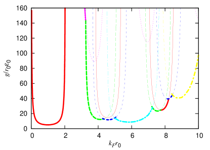
Figure 2: (color online) Phase diagram showing zero-temperature instabilities of the types depicted in Fig. 1 for the repulsive delta-shell model. The Stoner instability occurs above the solid line. The other instabilities described in Fig. 1 occur above the long dash line (b), medium dash line (c), short dash line (d), long dash-dot line (e) and short dash-dot line (f). The colors correspond with Fig.1

From point 4 we conclude that repulsive interactions with range at least of the order of the Fermi wavelength, $r_{0}\gtrsim k_{F}^{-1},$ are necessary for the PI in an isotropic system with isotropic interactions. We investigate this further by choosing a specific form of the central interaction potential, namely the “delta-shell” potential:

$$V\left(\left|\mathbf{r}\right|\right)=g\delta^{\left(1\right)}\left(\left|\mathbf{r}\right|-r_{0}\right).$$ (37)

This is an idealization of an interaction with a very sharp peak at a particular inter-particle distance, $\left|\mathbf{r}\right|=r_{0}.$ The “coupling constant” $g$ has dimensions of energy $\times$ length and represents the product of the height and width of the potential barrier.

For $g<0,$ this interaction potential can lead to superconductivity with unconventional pairing 2000-Quintanilla-Gyorffy ; quintanilla_02 . Likewise, we expect that for $g>0$ it will lead to a PI. Indeed Eq. (35) gives

$$V_{l}=\left(4\pi\right)^{2}gr_{0}^{2}j_{l}\left(k_{F}r_{0}\right)^{2}$$ (38)

so, depending on the value of $k_{F}r_{0},$ any value of $l$ may become dominant.

The particularly simple form of the interaction potential in Eq. (37) allows us to write the key expressions in our theory of the PI analytically. In particular Eq. (II) giving the Fermi velocity on the Fermi sphere reads

$$v_{F}=\frac{\hbar}{m}k_{F}+g\frac{2\left(k_{F}r_{0}\right)^{2}}{\hbar\pi}j_{1}\left(k_{F}r_{0}\right)^{2}.$$ (39)

Together with Eq. (38) and $\bar{V}=g4\pi r_{0}^{2}$ these equations allow us to write the following, simple form of the Stoner and PI equations:

$$j_{l}\left(k_{F}r_{0}\right)^{2}-j_{1}\left(k_{F}r_{0}\right)^{2}>\frac{\hbar^{2}}{2mr_{0}^{2}}\frac{\pi}{gk_{F}},\,l=0,1,2,\;\ldots$$ (40)

If the interaction is very strong, $gk_{F}\gg\hbar^{2}/2mr_{0}^{2},$ this gives a sequence of fixed phase boundaries at $j_{l}\left(k_{F}r_{0}\right)=\pm j_{1}\left(k_{F}r_{0}\right).$ In the opposite limit of very weak interaction the unpolarized Fermi sphere is, as expected, stable.

The solid, long dash and medium dash lines of Fig. 2 are the phase diagram obtained by solving Eq. (40) for $l\leq 3$. Note that there are effectively only two, dimensionless parameters in the theory 2000-Quintanilla-Gyorffy ; quintanilla_02 : the “effective range” $k_{F}r_{0}$ and “coupling constant” $g/r_{0}\varepsilon_{0}$ (where $\varepsilon_{0}=\hbar^{2}/2mr_{0}^{2}$). The first of these parameters is the range of the interaction measured in units of $1/k_{F}$. The second is the product of the width of the potential barrier measured in units of that range and its height measured in units of the corresponding “localization energy” $\varepsilon_{0}$. As expected, for small range, $k_{F}r_{0}\lesssim 3,$ we only find the Stoner instability. For longer ranges or, equivalently, higher densities, and sufficiently large values of the dimensionless coupling constant (which we note that depends not only on $g$ but also on $m$ and $r_{0}$), the PI can take place.

Figure 3: Electron dispersion relation for the “delta-shell” model in the state with an unpolarized Fermi sphere: (a) $k_{F}r_{0}=4$, $g/r_{0}\varepsilon_{0}=0\,(\textrm{solid}),\,20\,\textrm{(long dash)},\,97.66\,\textrm{(short dash)},\,150\,\textrm{(dotted)}$; (b) $k_{F}r_{0}=6$, $g/r_{0}\varepsilon_{0}=0,\,2,\,8.84,\,16$ (same order); (c) $k_{F}r_{0}=9$, $g/r_{0}\varepsilon_{0}=0,\,20,\,41.40,\,60$.

IV Topological transitions

In addition to the anticipated PI, our analytic treatment of the delta-shell model also reveals a competing class of Fermi surface instabilities which, unlike the PI, occur without symmetry breaking. Consider the electron dispersion relation in the isotropic state, Eq. (II). For the delta-shell potential it takes the form

$$\varepsilon\left(\left|\mathbf{k}\right|\right) = \frac{\hbar^{2}}{2m}\left(\left|\mathbf{k}\right|^{2}-k_{F}^{2}\right)-\frac{g}{r_{0}}\frac{2k_{F}^{2}r_{0}^{2}}{\pi}j_{1}\left(k_{F}r_{0}\right)$$

$$\left[j_{0}\left(\left|\mathbf{k}\right|r_{0}\right)-j_{0}\left(k_{F}r_{0}\right)\right].$$

This is plotted in Fig. 3 for three different values of $k_{F}r_{0}$. The free-electron dispersion relation is modified by an oscillatory term due to electron-electron interactions. The period of the oscillations is $\sim r_{0}^{-1}$. For small $g/r_{0}\varepsilon_{0}$ the effect of these is the usual renormalization of the effective mass $m^{*}=p_{F}/v_{F}$, which follows from Eq. (39). However at large $g/r_{0}\varepsilon_{0}$ the effect of interaction on this “bare” dispersion relation cannot be described simply as a renormalization of $m$. In fact it can lead to a dramatic change of the state of the system as the amplitude of the oscillations becomes large enough that either

1. the dispersion relation dips below the Fermi level somewhere outside the Fermi sphere [Fig. 3 (a)],

2. it goes above the Fermi level at the center of the Fermi sphere [Fig. 3 (b)] or

3. it peaks above the Fermi level at some intermediate $k$, $0<k<k_{F}$ [Fig. 3 (c)].

In either case, Eq. (27) no longer reduces to Eq. (30). Instead, either a thin shell of occupied states forms outside the Fermi sphere [Fig. 1 (d)], or states inside the Fermi sphere become vacated [Fig. 1 (e,f)]. The associated instabilities are quite distinct from the Stoner and PI, as the change $\delta N_{\mathbf{k},\sigma},$ although infinitesimal, takes place away from the Fermi surface. Instead, they are continuous phase transitions in which no symmetry is broken, but the topology of the Fermi surface changes. In that sense they are more reminiscent of the Lifshitz transition lifshitz ; lifshitz-2 . There is, however, a crucial difference, namely that the present phase transitions are driven by electron-electron interactions, which induce the fermions to “migrate” to other regions of reciprocal space, rather than by the band structure. On the basis of this one would expect the present instabilities to have a much stronger thermodynamic signature. For example, the transitions illustrated in Fig. 1(d) and (f), with their underlying dispersions of Fig. 3(a) and (c) respectively, result in the appearance of entire new Fermi surface sheets with finite $k_{F}$. This will lead in mean-field theory to a discontinuous jump in the density of states and hence in $C/T$.

Figure 4: Evolution of the Fermi vector as a function of the dimensionless coupling constant $g/r_{0}\varepsilon_{0}$ for fixed particle density $N/\Omega=9\leavevmode\nobreak\ r_{0}^{-3}$. The plot shows both the “original” Fermi vector $k_{F}$ and the “emerging” Fermi vector $k_{F}^{\prime}$, namely the radius of the sphere of empty states depicted in Fig. 1 (e), as the system enters from below the corresponding dome in the phase diagram (see Fig. 2).

A general framework to understand such topological quantum phase transitions has been put forward in Ref. 2006-Volovik, . In this formalism, the Fermi surface is a vortex “loop” in a four-dimensional space and the phase transitions we have just described correspond to the nucleation of new loops. One can also view these instabilities as generalizations to dimension larger than one of the phenomenon of “quantum Hall edge reconstruction”. The latter can be described as the emergence, due to interactions, of new Fermi points in the one-dimensional chiral Fermi liquid on the edge of a quantum Hall system 1993-MacDonald-Yang-Johnson ; 1994-Chamon-Wen ; 2002-Wan-Yang-Rezayi ; 2006-CastroNeto-Guinea-Peres . Indeed in the instabilities described here always one of the new Fermi surfaces has negative Fermi velocity - analogous to the creation of left-moving quasiparticles in a right-moving chiral Fermi liquid . Yang and Sachdev 2006-Yang-Sachdev have recently described the quantum critical fluctuations for a phase transition of type 1, above [Figs. 1 (d) and  3 (a)].

It is important to note that the plots in Fig. 3 correspond to evaluating Eq. (IV) at a fixed value of $k_{F}$. For a fixed number of particles, $N$, such solutions are valid only up to the instability, as beyond it they would violate Luttinger’s theorem. To describe the migration of electrons in reciprocal space mentioned above, which happens beyond the instability, it is necessary to determine $k_{F}$ self-consistently by requiring that the total number of particles be fixed. For example, for an instability of the type 2, above [Figs. 3 (b) and 1 (e)], this means that

$$\frac{N}{\Omega}=2\frac{1}{(2\pi)^{3}}\frac{4\pi}{3}\left(k_{F}^{3}-k_{F}^{\prime 3}\right),$$ (42)

where $k_{F}^{\prime}$ is the “emerging” Fermi vector at the centerer of the Fermi sphere, determined by $\varepsilon(k_{F}^{\prime})=0$. This is demonstrated in Fig. 4. Note that the way $k_{F}^{\prime}$ grows as a function of coupling suggests thinking of this quantity as a sort of topological “order parameter”.

It is evident from Fig. 3 that the new sheet of electron-like or hole-like Fermi surfaces are initially formed by localized states, with $v_{F}=0.$ As we progress into the new state, $v_{F}$ becomes finite. Conversely, if we run the process backward, the effective masses on the additional Fermi surfaces diverge (except for the hole-like Fermi surface in Fig. 1 (e), for which the Fermi vector goes to zero at the same time as the Fermi velocity).

The short dash, long dash-dot and short dash-dot lines on Fig. 2 show the boundaries of these “Fermi surface topology transitions”. Notably, except for a range of densities near where the $l=1$ PI would have been, the unpolarized Fermi sphere is only stable at small coupling

V Hard-core model

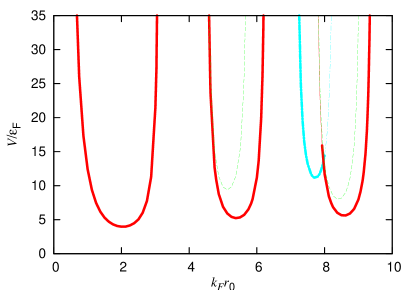
Figure 5: (color online) Phase diagram showing zero-temperature instabilities of the unpolarized, spherical Fermi surface for the “hard-core” model. The coupling constant is measured in units of the Fermi energy $\varepsilon_{F}=\hbar^{2}k_{F}^{2}/2m$. Key as in Fig.2.

Our results suggest that the essential ingredient of the PI in the present context, namely the finite range $r_{0}\sim k_{F}^{-1}$, also leads to the interaction-driven Lifshitz transition. To probe the generality of this observation, we have repeated the calculation (this time by evaluating the mean-field equations (II) and (34) numerically) for a repulsive “hard core” potential

$$V\left(\left|\mathbf{r}\right|\right)=V\Theta\left(r_{0}-\left|\mathbf{r}\right|\right).$$ (43)

We have again found that, for $r_{0}\gtrsim k_{F}^{-1},$ there are, in addition to the Stoner instability, PI with $l=2,4,6,\ldots$ Moreover we also find an interaction-driven Lifshitz transition which, for certain ranges of values of $k_{F}r_{0}$, takes place before the Stoner or PI set in. A phase diagram is presented in Fig. 5.

Unlike the delta-shell potential, for the hard core potential the PI domes are contained within the Stoner ones, i.e. the PI can only take place on a polarized Fermi surface, or for spinless fermions. However note that there are regions of the phase diagram where the boundary of the $l=2$ instability nearly overlaps with that for $l=0$, indicating that the two transitions happen almost simultaneously.

The plot does not show all the instabilities: the $l>2$ PI take place at higher values of $k_{F}r_{0}$ than those shown. The are also other domes of topological instability, though for this potential all of them are of the type in Fig.1 (e).

Our results for the hard-core potential not only support our identification of a sharp feature of $V\left(r\right)$ at $r_{0}\sim k_{F}^{-1}$ as the crucial ingredient for a PI, but suggest as well that, in such situations, the interaction-driven Lifshitz transition is at least as likely to occur as the Stoner or PI.

We conclude this section by noting that a similar analysis using the screened Coulomb interaction

$$V\left(\left|\mathbf{r}\right|\right)=\frac{e^{2}}{4\pi\epsilon_{0}^{2}}\frac{e^{-\left|\mathbf{r}\right|/r_{0}}}{\left|\mathbf{r}\right|}$$ (44)

does not reveal either PI or instabilities of the Fermi surface topology —only the Stoner instability is realized, and that only if we allow $r_{0}$ to deviate from its Thomas-Fermi value.

VI Conclusions

In summary we have studied, at the mean field level, PI of a uniform Fermi liquid with central fermion-fermion interactions. We find that PI of different symmetries may emerge from repulsive interactions of sufficiently long, but finite range $r_{0}\gtrsim k_{F}^{-1}$ (with the interesting exception of the $l=1$ PI which never takes place). We have confirmed this by solving the theory analytically for an explicit form of the interaction potential featuring repulsion at a particular distance $r_{0}$. Surprisingly we have found that, in addition to the PI, there is also a new type of Fermi surface instability: the interaction-driven Lifshitz transition. This topological phase transition is even subtler than the PI and seems to be generically associated with the class of models leading to the PI. Further support for this picture is provided by analysis of an additional model, featuring hard-core repulsion. On the other hand the screened Coulomb interaction does not lead to these effects suggesting that a sharp feature (either a spike of repulsion or a sudden drop) must be present at the distance $r_{0}$.

Unlike the Lifshitz transition, the new quantum phase transition that we have described is fundamentally driven by interactions. Thus one would expect it to have a stronger thermodynamic signature. It will be of great interest, in the near future, to establish this signature and the properties of the novel state of matter this phase transition may lead to.

- (1) J. L. Tallon et al., Phys. Stat. Sol. (b) 215, 531 (1999).
- (2) T. T. M Palstra et al., Phys. Rev. Lett. 55, 2727 (1985); M. B. Walker et al., Phys. Rev. Lett. 71, 002630 (1993); K. H. Kim et al., Phys. Rev. Lett. 91, 256401 (2003).
- (3) S. A. Grigera et al., Science 306, 1154 (2004).
- (4) L. Balicas et al., Phys. Rev. Lett. 87, 067002 (2001).
- (5) J. F. Annett, M. Krawiec and B. L. Gyorffy, cond-mat/0510591.
- (6) T. Mizushima et al., Phys. Rev. Lett. 94, 060404 (2005).
- (7) Kun Yang, Phys. Rev. Lett. 95, 218903 (2005).
- (8) K. Góral, L. Santos and M. Lewenstein, Phys. Rev. Lett. 88, 170406 (2002).
- (9) S. Chakravarty, R. B. Laughlin, D. K. Morr and C. Nayak, Phys. Rev. B 63, 094503 (2001).
- (10) U. Schollowöck et al., Phys. Rev. Lett. 90, 186401 (2003).
- (11) S. Lee, J. B. Marston and J. O. Fjaerestad, Phys. Rev. B 72, 075126 (2005).
- (12) I. Ia. Pomeranchuk, JETP 35, 524-525 (1958).
- (13) E. Fradkin and S. A. Kivelson, Phys. Rev. B 59, 8065 (1999).
- (14) E. Fradkin, S. A. Kivelson, E. Manousakis and K. Nho, Phys. Rev. Lett. 84, 1982 (2000).
- (15) C. M. Varma and Lijun Zhu, cond-mat/0502344.
- (16) C. J. Halbloth and W. Metzner, Phys. Rev. Lett. 85, 5162 (2000).
- (17) V. Hankevych, I. Grote and F. Wegner, Phys. Rev. B 66, 094516 (2002).
- (18) W. Metzner, D. Rohe and S. Andergassen, Phys. Rev. Lett. 91, 066402 (2003).
- (19) A. Neumayr and W. Metzner, Phys. Rev. B 67, 035112 (2003).
- (20) E. C. Carter and A. J. Schofield, Phys. Rev. B 70, 045107 (2004).
- (21) The PI may also be favored by non-linearities in the electron dispersion relation: D. G. Barci and L. E. Oxman, Phys. Rev. B 67, 205108 (2003).
- (22) S. A. Kivelson, E. Fradkin and T. H. Geballe, Phys. Rev. B 69, 144505 (2004).
- (23) Hae-Young Kee and Yong Baek Kim, Phys. Rev. B 71, 184402 (2005).
- (24) I. Khavkine, Chung-Hou Chung, V. Oganesyan and Hae-Young Kee, Phys. Rev. B 70, 155110 (2004).
- (25) H. Yamase, V. Oganesyan and W. Metzner, Phys. Rev. B 72, 35114 (2005).
- (26) V. Oganesyan, S. A. Kivelson and E. Fradkin, Phys. Rev. B 64, 195109 (2001).
- (27) Hae-Young Kee, Phys. Rev. B 67, 073105 (2003).
- (28) J. Nilsson and A. H. Castro Neto, Phys. Rev. B 72, 195104 (2005).
- (29) L. Dell’Anna and W. Metzner, cond-mat/0507532.
- (30) M. J. Lawler et al., cond-mat/0508747.
- (31) C. M. Varma, Phil. Mag. 85, 1657-1666 (2005).
- (32) A. J. Leggett, Rev. Mod. Phys. 47, 331 (1975).
- (33) S. A. Kivelson, E. Fradkin and V. J. Emery, Nature 393, 550 (1998).
- (34) P. Nozières and S. Schmitt-Rink, J. Low. Temp. Phys. 59, 195 (1985).
- (35) P. Nozieres, J. Phys. I France 2, 443-458 (1992).
- (36) Congjun Wu and Shou-Cheng Zhang, Phys. Rev. Lett. 93, 36403 (2004).
- (37) J. Quintanilla and B. L. Gyorffy, Physica B 284-288, 421-422 (2000).
- (38) J. Quintanilla, B. L. Gyorffy, J. F. Annett and J. P. Wallington, Phys. Rev. B 66, 214526 (2002).
- (39) I. M. Lifshitz, Zh. Eksp. Teor. Fiz. 38, 1569 (1960) [Sov. Phys. JETP 11, 1130 (1960)].
- (40) A. A. Abrikosov, “Fundamentals of the Theory of Metals” (Elsevier, New York, 1988).
- (41) G. Volovik, cond-mat/0601103.
- (42) A. H. MacDonald, S. R. Eric Yang and M. D. Johnson, Aust. J. Phys. 46, 345 (1993).
- (43) C. de C. Chamon and X. G. Wen, Phys. Rev. B 49, 8227 ( 1994).
- (44) Xin Wan, Kun Yang and E. H. Rezayi, Phys. Rev. Lett. 88, 056802 (2002).
- (45) A. H. Castro Neto, F. Guinea and N. M. R. Peres, Phys. Rev. B 73, 205408 (2006).
- (46) Kun Yang and Subir Sachdev, Phys. Rev. Lett. 96, 187001 (2006).
- (47) C.M. Varma, Phys. Rev. B 55, 14554 (1997); Phys. Rev. Lett. 83, 3538 (1999).
- (48) B. Fauque, Y. Sidis, V. Hinkov, S. Pailhes, C. T. Lin, X. Chaud, and P. Bourges, Phys. Rev. Lett. 96, 197001 (2006).