Electrical Detection of Self-Assembled Polyelectrolyte Multilayers by a Thin Film Resistor

Abstract

The build up of polyelectrolyte multilayers (PEMs) was observed by a silicon-on-insulator (SOI) based thin film resistor. Differently charged polyelectrolytes adsorbing to the sensor surface result in defined potential shifts, which decrease with the number of layers deposited. We model the response of the device assuming electrostatic screening of polyelectrolyte charges by mobile ions within the PEMs. The screening length $\kappa^{-1}$ inside the PEMs was found to be increased compared to the value corresponding to the bulk solution. Furthermore the partitioning of mobile ions between the bulk phase and the polyelectrolyte film was employed to calculate the dielectric constant of the PEMs and the concentration of mobile charges.

Introduction. Despite the broad potential applications of polyelectrolyte multilayers (PEMs) a detailed understanding of the build up process and the resulting basic physical properties is still elusive. While the multilayer thickness, the water content, the mechanical properties and the swelling behavior of different PEMs systems have been extensively studied, their electrostatic properties are still not fully determined. PEMs are prepared by the layer–by–layer deposition of polyanions and polycations from aqueous solutions [1, 2]. During the adsorption process polyanion/polycation complexes are formed with the previously adsorbed polyelectrolyte layer [3] leading to a charge reversal [4]. The exchange of counterions by the oppositely charged polyelectrolyte could be the reason for the counterion concentration inside the PEMs to be below the detection limit [5]. Thus, it seems that most of the charges within the PEMs are compensated intrinsically by the opposite polymer charges and not by the presence of small counterions. Related to the intrinsic charge compensation may be the strong interdigitation between adjacent layers found by neutron reflectometry [6, 7]. While the potential of the outer PEMs surface is well investigated by electrokinetic measurements [4], not much is known about the internal electrostatic properties like ion distribution and mobility. Using a pH-sensitive fluorescent dye the distribution of protons within the PEMs has been determined [8]. Assuming Debye screening and a constant mobility for all ions within the PEMs the potential drop within polyelectrolyte films composed of poly(allylamine hydrochloride) (PAH) and poly(sodium 4-styrenesulfonate) (PSS) has been calculated. From these measurements an independent determination of the ionic strength and the dielectric constant was not possible. Recent X–ray fluorescence measurements have been promising in estimating the ion density profile inside the PEMs giving the total amount of free and condensed ions [9].

Direct measurements of the potential drop inside the PEMs will be best suited for determining electrostatic properties such as the Debye length or the dielectric constant of the PEMs. The capacitance of the PEMs can be measured by electrochemical methods such as AC voltammetry [10]. Another approach is the use of field effect devices which allows the determination of the surface potential at the sensor/electrolyte interface. Obviously, the surface potential variations measured by such a device are strongly dependent on screening effects inside the adjacent phase. The deposition of PAH/PSS as well as poly(L-lysine)/DNA multilayers and even DNA hybridization have been detected by such devices [11, 12, 13]. However, a physical model is needed to relate the quantitative response of the sensors to the dielectric properties and ion mobility inside the PEMs.

Here we show that a silicon-on-insulator (SOI) based thin film resistor is suited to monitor in real time the build up of polyelectrolyte multilayers consisting of the strong polyelectrolyte PSS and the weak polyelectrolyte PAH. The sheet resistance of the field effect device is sensitive to variations of the potential $\psi_{\mathrm{S}}$ at the silicon oxide surface. The deposition of the differently charged polyelectrolytes results in defined potential shifts, which decrease with the number of layers deposited. Applying a capacitor model, the observed decrease can be quantitatively explained by assuming reduced electrostatic screening by mobile charges inside the PEMs compared to the bulk medium outside.

Experimental Section. All chemicals including PSS (MW 70,000) and PAH (MW 60,000) were purchased from Sigma-Aldrich. Buffers were prepared using ultrapure water (Millipore, France) with a resistivity $>18$ M$\Omega$ cm. 5 mg/ml polyelectrolyte solutions were prepared by direct dissolution in $10$ mM Tris buffer at pH 7.5 containing $50$ and $500$ mM NaCl, respectively.

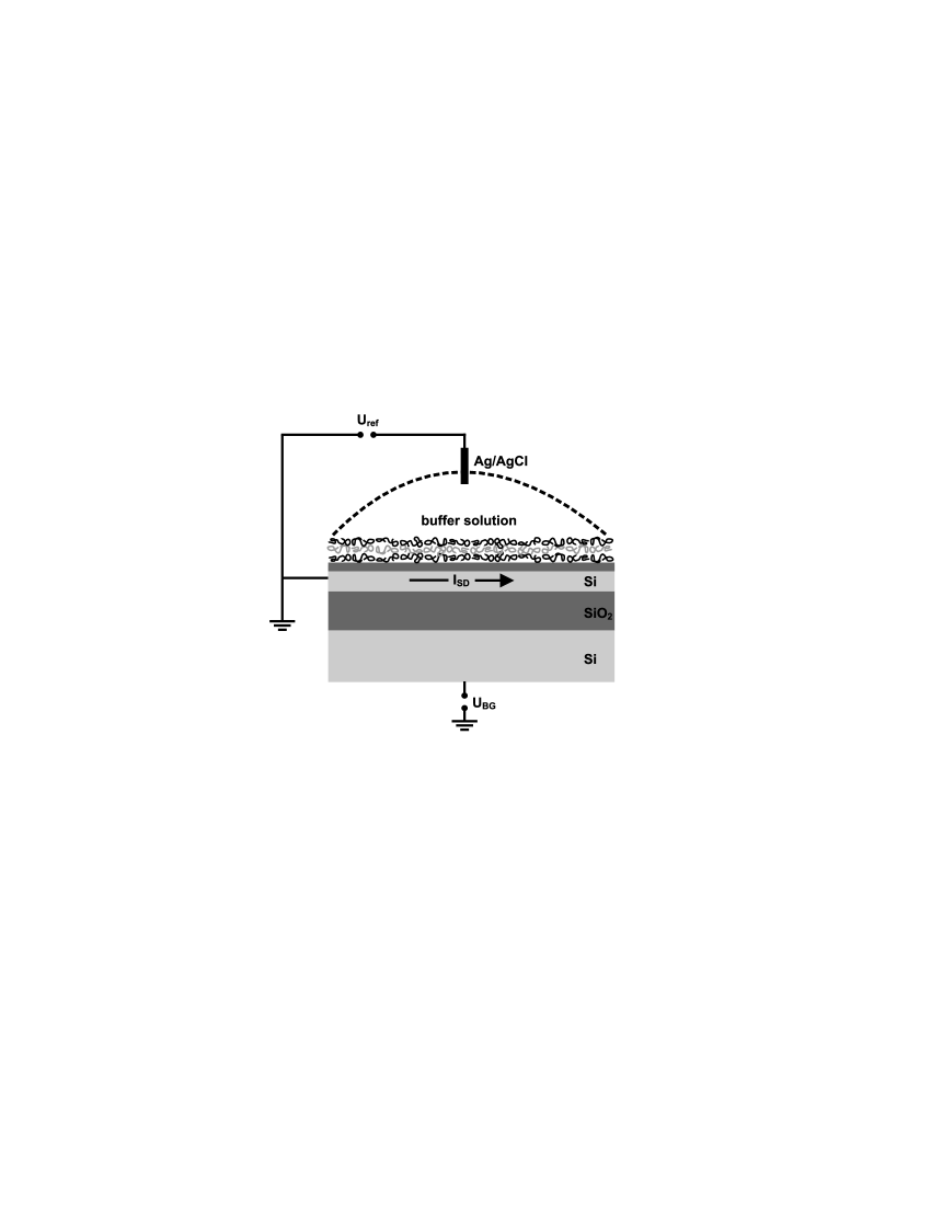
Figure 1: Sketch of the setup and the measurement geometry. Silicon is shown in light grey, silicon oxide in dark grey. From top to bottom: native oxide (1-2 nm), conducting top silicon (30 nm), buried oxide (200 nm), bulk silicon (675 $\mu$m). A voltage is applied between the source and the drain contacts and the resulting current $I_{\text{SD}}$ is measured yielding the sheet resistance of the device. The carrier concentration in the top silicon layer is tuned by the backgate voltage $U_{\text{BG}}$. The potential of the electrolyte solution is controlled by a Ag/AgCl reference electrode. A microfluidic device allows the rapid exchange of electrolyte solution.

The sensor chips were fabricated from commercially available silicon-on-insulator (SOI) wafers (ELTRAN, Canon) using standard lithographic methods and wet chemical etching as described in detail elsewhere [14]. The top silicon layer of these wafers was 30 nm thick and slightly doped with boron ($10^{16}$ cm^-3). Metal contacts were deposited in an electron beam evaporation chamber (20 nm Ti, 300 nm Au). After evaporation, the sensor chips were cleaned using acetone and isopropanol. The chips were glued into a chip carrier and the contacts were Au-wire bonded to the carrier. Afterwards the chips were encapsulated with a silicone rubber to insulate the contacts from the electrolyte solution. The sheet resistance of the device is dependent on the potential $\psi_{\mathrm{S}}$ of the SiO_x/PEMs interface and was measured as described elsewhere [15]. The potential $\psi_{\mathrm{S}}$ was then calculated from the sheet resistance by a calibration curve of the specific SOI wafer. A flow chamber was mounted on top of the sensor and a Ag/AgCl reference electrode was used to control the potential of the electrolyte solution and for calibration. The setup and the measurement geometry are shown schematically in Figure 1. First, the sensor was equilibrated in the buffer solution. Next, a calibration measurement was performed as shown elsewhere [15]. PAH and PSS solutions were injected twice into the flow chamber to insure full coverage of the sensor surface, starting with the positively charged PAH. After obtaining a stable sensor signal, the chamber was rinsed twice with buffer of the same salt concentration as the polyelectrolyte solutions. As soon as a stable signal was obtained, the next polyelectrolyte solution was injected and the procedure was repeated up to 20 times. The sheet resistance of the thin film resistor was monitored continuously during the multilayer deposition. In separate experiments the thickness of the deposited polyelectrolyte films was determined by an ellipsometer (Optrel, Multiscope, Berlin, Germany) in electrolyte solution. Care was taken to perform the preparation of multilayers as close as possible to the conditions employed for the deposition on the thin film resistors. The ellipsometry was carried out in the same buffer solutions used for the sample preparation.

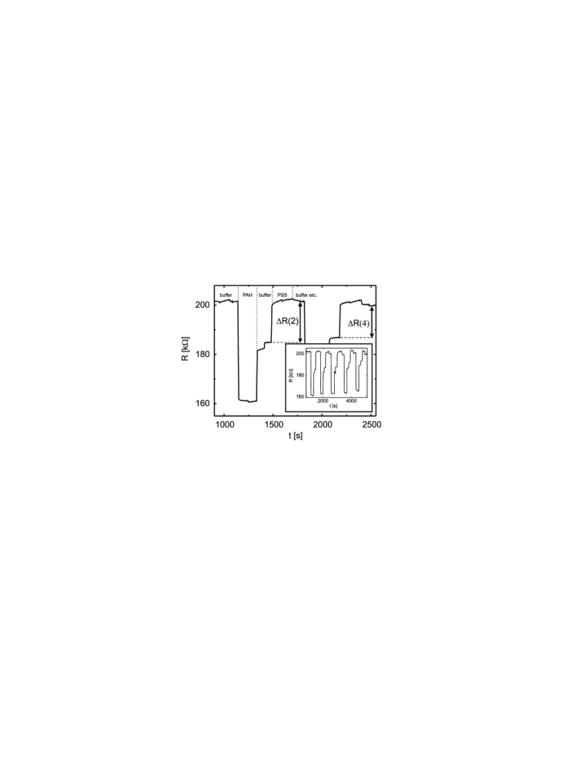
Figure 2: The deposition of four PEMs from 50 mM NaCl is shown in detail. The sheet resistance was monitored continuously during the build-up process. For each deposition step the polyelectrolyte solution was injected twice. When a stable signal was obtained the sensor was rinsed twice with buffer. The resistance change $\Delta R$ between adjacent deposition steps of PAH and PSS is indicated for two and four adsorbed layers. The potential change between adjacent deposition steps $\Delta\psi_{\mathrm{S}}$ was calculated from $\Delta R$ using the calibration data. The inset displays the subsequent adsorption of 10 layers.

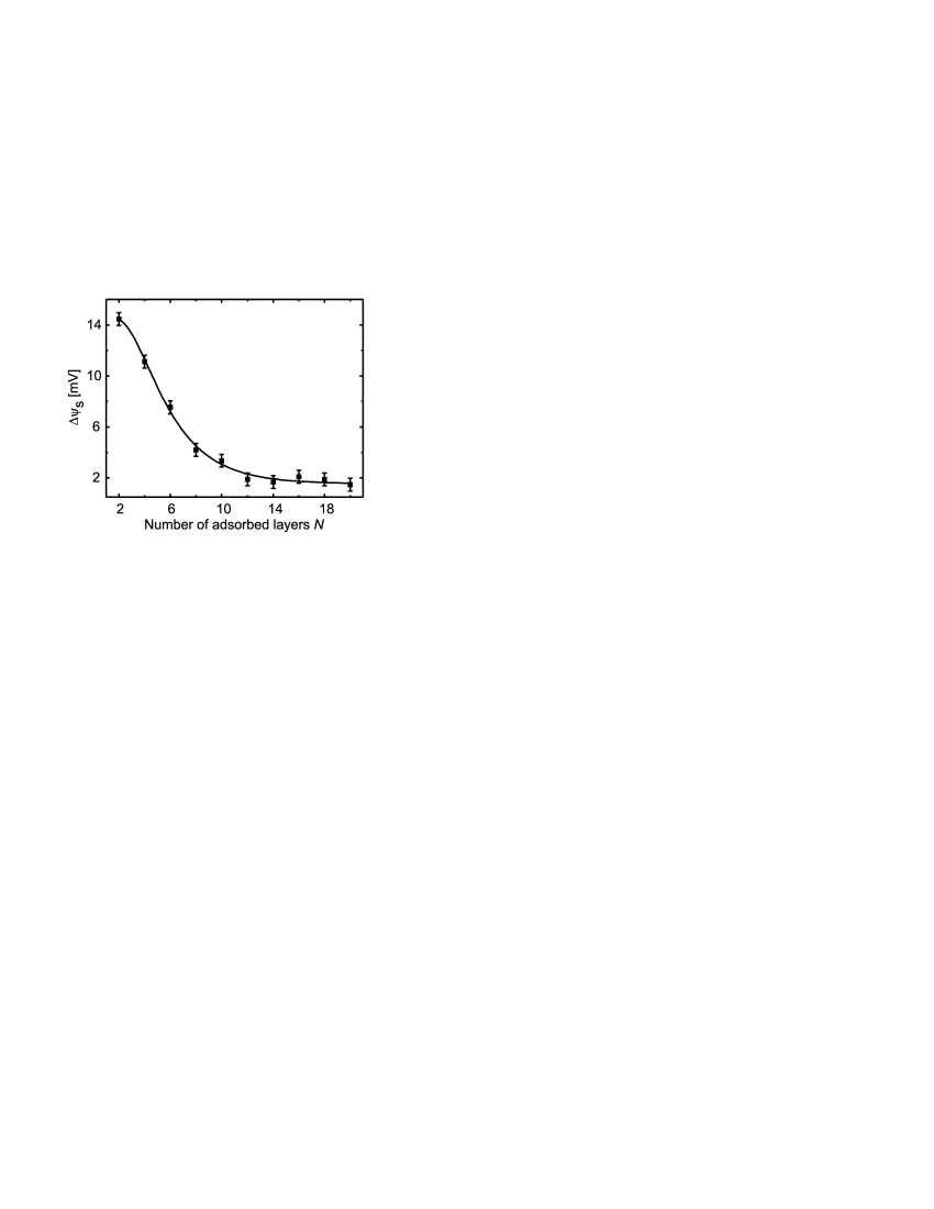
Figure 3: The potential change $\Delta\psi_{\text{S}}$ calculated from the measured change in sheet resistance is plotted as a function of the number of adsorbed monolayers $N$ for PEMs deposited from 500 mM NaCl. Error bars are determined from the peak to peak noise of the measurement. Applying the capacitor model the solid curve was obtained from the fit by Eq. (1).

Results and Discussion. During the layer-by-layer deposition of the polycation PAH and the polyanion PSS by alternating buffer exchange, the sheet resistance of the SOI sensor was continuously observed. The deposition of the alternately charged polyelectrolytes results in defined responses of the sensor (Figure 2). The adsorption of PAH decreases the sheet resistance corresponding to an increased $\psi_{\mathrm{S}}$ (the potential directly at the SiO_x/PEMs interface) as positive charges bind to the surface. The subsequent adsorption of the negatively charged PSS increases the resistance and thus decreases $\psi_{\mathrm{S}}$. As the SOI sensor exhibits also a pH sensitivity [15], the large potential shift between the PAH deposition and the subsequent washing step can be attributed to the pH of the PAH solution which is decreased to 6.4 by dissolution of the week polyelectrolyte in the buffer of pH 7.5. The deposition of up to 20 monolayers was observable by the field effect device. The potential change between adjacent deposition steps $\Delta\psi_{\mathrm{S}}$ was determined from the measured sheet resistance using the calibration data and is plotted against the number of adsorbed monolayers as shown in Figure 3. It can clearly be seen that the potential jumps $\Delta\psi_{\mathrm{S}}$ decrease with the number of layers deposited. This is in contrast to electrokinetic studies, where the surface potential at the outer PEMs/electrolyte interface is measured and the steps remain constant over a large number of deposited layers [4]. The observed decrease of $\Delta\psi_{\mathrm{S}}$ can be explained by adapting a capacitor model [10, 16]. The sensor device with the adsorbed PEMs is modelled assuming three separate domains: (i) The sensor device, which is modelled as a one dimensional silicon/silicon oxide structure characterized by its capacitance per area $C_{\mathrm{S}}$. (ii) The PEMs consisting of $N$ monolayers each of thickness $d$. (iii) The electrolyte solution outside the PEMs, where a diffuse electrical double layer is formed at the PEMs/electrolyte interface (Figure 4). In order to proceed we need to model the charge distribution within the PEMs. In general, the layers have a complex charge distribution due to, for example, interdigitation between polymers from adjacent layers. This overlapping of layers can even be of the same order as the layer thickness [7] suggesting charge neutralization within the PEMs [5]. Therefore, we consider two limiting cases (Figure 4): a) separate layers inside the PEMs with uniform volume charge density of $\rho=\pm\frac{\sigma}{d}$, where $\sigma$ may be regarded as the surface charge density of each layer, and b) overlapping layers such that polyelectrolyte charges are completely neutralized within the PEMs, and thus the only uncompensated charges occur at the sensor surface and the PEMs/electrolyte interface with the surface charge density of $\pm\frac{\sigma}{2}$. Electrostatic screening by mobile charges is accounted for using the linear Debye-Hückel (DH) theory both within the PEMs medium (which is characterized by the screening length $\kappa^{-1}$ and the dielectric constant $\varepsilon$) as well as in the diffuse electrical double layer of the electrolyte solution (which is characterized by the bulk screening length $\kappa_{0}^{-1}$ and the dielectric constant for water $\varepsilon_{\mathrm{w}}$). One can thus identify characteristic Debye capacitances per area of $C_{\mathrm{P}}=\varepsilon\varepsilon_{0}\kappa$ and $C_{\mathrm{D}}=\varepsilon_{\mathrm{w}}\varepsilon_{0}\kappa_{0}$ for the two media, respectively. The two models a and b considered for the limiting cases described above yield similar results for the behavior of $\psi_{\mathrm{S}}$. On the linear Debye-Hückel level even identical results are obtained, indicating that the precise charge distribution within the PEMs is not a critical factor in our model (see Supporting Information). To compare our measurements with the model predictions, we calculate $\Delta\psi_{\mathrm{S}}=\psi_{\mathrm{S}}(N-1)-\psi_{\mathrm{S}}(N)$ which can be simplified for $\kappa d\ll 1$ and even number of layers, $N$, yielding

$$\Delta\psi_{\mathrm{S}}(N)=\frac{\sigma\,C_{\mathrm{D}}^{-1}}{\left(C_{\mathrm{S}}/C_{\mathrm{P}}+C_{\mathrm{P}}/C_{\mathrm{D}}\right)\sinh\left(\kappa Nd\right)+\left(1+C_{\mathrm{S}}/C_{\mathrm{D}}\right)\cosh\left(\kappa Nd\right)}.$$ (1)

In Eq. (1) the number of layers, $N$, appears only in the hyperbolic functions. A value for the screening length $\kappa^{-1}$ inside the PEMs can be obtained from the measured potential change $\Delta\psi_{\mathrm{S}}(N)$ if the thickness $d$ of the polyelectrolyte layers at a given ionic strength is known. Therefore the monolayer thickness $d$ was independently measured by ellipsometry. We found an average thickness of $d=1.3\pm 0.1$ nm for deposition from 50 mM and $d=2.2\pm 0.1$ nm for deposition from 500 mM bulk electrolyte solution, respectively. Selected ellipsometry data have been crosschecked by X–ray synchrotron reflectivity experiments [18] confirming the obtained PEMs thicknesses. As can be seen in Figure 3, the measured $\Delta\psi_{\mathrm{S}}$ can be fitted for $\kappa d$ by Eq. (1), yielding $\kappa^{-1}=6.5\pm 1.0$ nm for 500 mM bulk solution. A similar fit results in $\kappa^{-1}=6.3\pm 1.0$ nm for the build up of the PEMs at 50 mM bulk solution. Eq. (1) also provides an estimate for the surface charge density $\sigma$ of the adsorbed polyelectrolyte layers, assuming that $C_{\mathrm{S}}$ is much smaller than $C_{\mathrm{D}}$ ($1+C_{\mathrm{S}}/C_{\mathrm{D}}\approx 1$). This leads to $\sigma=0.020\leavevmode\nobreak\ \frac{\mathrm{C}}{\mathrm{m}^{2}}$ for the adsorption from 50 mM and $\sigma=0.022\leavevmode\nobreak\ \frac{\mathrm{C}}{\mathrm{m}^{2}}$ from 500 mM bulk solution.

The relative dielectric constant $\varepsilon$ of the PEMs can be calculated from $\kappa$, given the definition $\kappa^{2}=2N_{\mathrm{A}}e^{2}c/(\varepsilon\varepsilon_{0}kT)$, where $N_{\mathrm{A}}$ is Avogadro’s number, $e$ is the elementary charge, $c$ is the ion concentration, and $k$ is the Boltzmann constant. For this, one has to determine the concentration $c$ of mobile ions inside the PEMs, which is set by the thermodynamic equilibrium between the ions in the bulk solution (of concentration $c_{0}$) and those in the PEMs (see Supporting Information for details). It turns out that the dominant factor governing the ion-partitioning in the PEMs/bulk electrolyte system is the Born energy change,

$$\Delta\mu=\frac{e^{2}}{8\pi\varepsilon_{0}a}\left[\frac{1}{\varepsilon}-\frac{1}{\varepsilon_{\mathrm{w}}}\right],$$ (2)

which arises because of the difference in self-energy of the ions (of radius $a$) in the PEMs and in the bulk leading to the well-known ion-partitioning law $c=c_{0}\exp(-\Delta\mu/kT)$ [19, 20]. Combining the preceding relations and the definition of $\kappa$, the relative dielectric constant $\varepsilon$ of the PEMs and the concentration of mobile ions can be calculated numerically from the values obtained for $\kappa$. We find $\varepsilon=30\pm 2$ and $\varepsilon=21\pm 1$ for the multilayers adsorbed from 50 mM NaCl and 500 mM NaCl, respectively. The corresponding concentration of mobile ions inside the PEMs is estimated to be of the order $0.9\pm 0.3$ mM and $0.6\pm 0.2$ mM, respectively.

A slightly higher value of $\varepsilon=50\pm 10$ for the relative dielectric constant of PAH/PSS films has been estimated by comparing pyrene fluorescence data of the films with that of various isotropic solvents of low molecular weight [21]. Durstock and Rubner [22] found dielectric constants by factor 20 higher for PAH/PSS multilayers in water vapor. The large deviation from the values of the present paper is not fully understood. A possible explanation could be differences in swelling behavior in water vapor and liquid water as shown by neutron reflectometry.

The different values for $\varepsilon$ obtained for PEMs deposited from different salt concentrations can be interpreted in terms of a different water content of the polyelectrolyte films. A water content of about 40% was estimated by neutron reflectometry for PAH/PSS films deposited from different salt concentrations [7, 23, 24, 25] suggesting that the ionic strength of the solution does not change the water content of the PEMs. Assuming an equal water content for both salt concentrations the observed variation of the dielectric constant could be ascribed to a different fraction of immobilized to free water within the polymer layers as oriented water molecules show a lower dielectric constant. Decreased water mobility inside PEMs has already been determined by NMR studies [26]. Comparing measurements at different conditions will be necessary to further determine the origin of the dielectric constants of PEMs.

Note that the DH approximation used in the present theoretical model is valid for relatively small electrostatic potentials. At room temperature, for symmetrical monovalent electrolytes this yields an upper limit of 50 mV, which is typically larger than the potentials measured in our experiments. In general a full non-linear Poisson-Boltzmann analysis would be necessary, which, however, is not analytically solvable for the present system. The main advantage of the DH approach lies in obtaining a simple analytical expression for the sensor device functionalized by PEMs enabling a direct comparison with the experimental data.

Conclusion. We were able to show that the recently introduced field effect device based on SOI is well suited for the quantitative determination of charge variations at complex interfaces. We apply a capacitor model including electrostatic screening by mobile charges within the PEMs to determine their dielectric constant as well as the concentration of mobile ions inside the polymer film. The origin of the dielectric constants found for PEMs deposited from different salt concentrations will need to be addressed further. The presented theoretical description, which is given here for the PEMs, may prove useful also for the quantitative analysis of differently functionalized field effect devices.

Acknowledgment. This work was funded by the Deutsche Forschungsgemeinschaft within the SFB 563 and partially by the French–German Network and by the Fonds der Chemischen Industrie. The authors thank Roland Netz for helpful scientific discussions.

Supporting Information Available: Details of the capacitor models and the thermodynamic equilibrium between the ions in the bulk solution and the PEMs are given. This material is available free of charge via the Internet at http://pubs.acs.org.

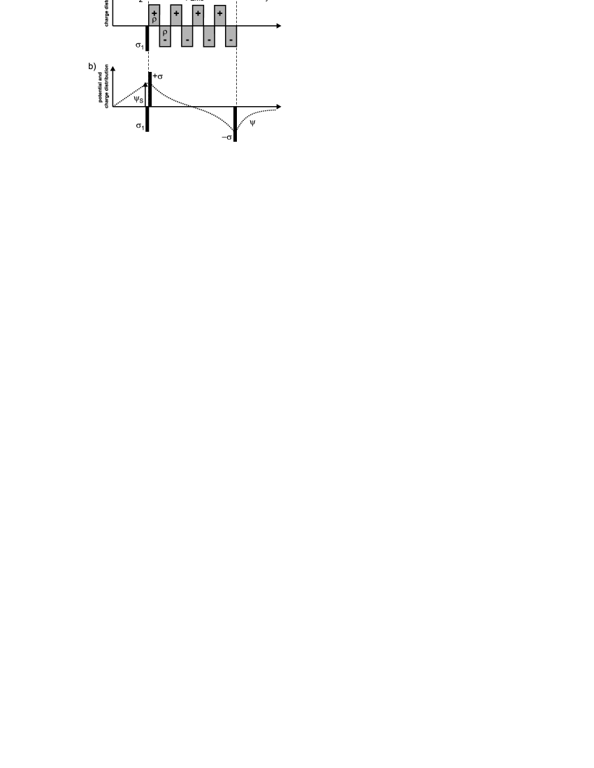
Figure 4: The system is modeled using three separate domains: (i) the Si/SiO₂ structure, (ii) the PEMs, and (iii) the electrolyte solution. The distribution of the immobile charges (the polyelectrolyte charges and the silicon oxide surface charge $\sigma_{1}$) is shown for two limiting cases: a) separate layers inside the PEMs with a volume charge density $\rho$ and b) overlapping layers inside the PEMs with neutralized charges except for the charges at the sensor surface and the PEMs/electrolyte interface with the surface charge density of $\pm\frac{\sigma}{2}$. Volume charges $\rho$ are displayed in grey whereas surface charges $\sigma$ are displayed in black. For case b) the dotted line schematically shows the potential within the system. The potential $\psi_{\text{S}}$ at the sensor surface is indicated.

Supporting Information

Theoretical models for the detection of polyelectrolyte multilayers by the SOI-based thin film resistor

Model a: Alternating layers with volume charges

We model the polyelectrolyte multilayers sensor system as a series of $N$ alternately positively and negatively charged layers with the volume charge distribution $\rho=\pm\frac{\sigma}{d}$ (Figure 4a, main text). The potential in the silicon/silicon oxide structure is assumed to be linear. It is determined by the capacitance per area of the device $C_{\mathrm{S}}=\frac{\varepsilon_{1}}{d_{1}}$ which is given by the effective dielectric constant $\varepsilon_{1}$ and the thickness $d_{1}$. The charge of the silicon oxide surface is given by $\sigma_{1}.$ In the PEMs, the Debye-Hückel (DH) equation

$$\frac{\mathrm{d}^{2}}{\mathrm{d}x^{2}}\psi\left(x\right)-\kappa^{2}\psi\left(x\right)=-\frac{1}{\varepsilon}\rho\left(x\right)$$

is solved for each single polyelectrolyte layer with $\rho\left(x\right)=\pm\frac{\sigma}{d}$. The screening length inside the PEMs is assumed to be $\kappa^{-1}$ and the dielectric constant is $\varepsilon$. The diffuse electrical double layer in the electrolyte is described by the dielectric constant for water $\varepsilon_{\mathrm{w}}$ and the screening length $\kappa_{0}^{-1}$ which is equal to the effective double layer thickness. The actual distribution of counterions at the charged surface is diffuse and reaches the unperturbed bulk value only at large distances from the surface, which is described by an exponential decay of the potential. However, a diffuse double layer behaves like a parallel plate capacitor in which the separation between the plates is given by the screening length $\kappa_{0}^{-1}$. Thus we can describe the potential within the electrolyte by a plate capacitor with the Debye capacitance per area $C_{\mathrm{D}}=\varepsilon_{\mathrm{w}}\varepsilon_{0}\kappa_{0}$. The surface charges $\sigma_{0}$ and $\sigma_{L}$ represent the space charges within the seminconductor and the electrical double layer of the electrolyte, respectively. The potential difference between the bulk semiconductor and the bulk electrolyte is $U_{\mathrm{tot}}$ and is set by the reference electrode. The potential $\psi$ within the $N+2$ domains (i), (ii)₁, …, (ii)${}_{N},$ and (iii) is given by

$$\psi_{\text{(i)}}\left(x\right) = A^{\prime}x+A,$$

$$\psi_{\text{(ii)}_{n}}\left(x\right) = C_{n}\exp\left(-\kappa x\right)+D_{n}\exp\left(\kappa x\right)+\psi_{n}\left(x\right),\qquad n=1,\ldots,N$$

$$\psi_{\text{(iii)}}\left(x\right) = B^{\prime}x+B,$$

where $C_{n}\exp\left(-\kappa x\right)+D_{n}\exp\left(\kappa x\right)$ is the general solution of the homogeneous DH equation and $\psi_{n}\left(x\right)$ is a particular solution of the inhomogeneous DH equation for $\rho\left(x\right)=-\frac{\sigma}{d}\left(-1\right)^{n}$. We apply the following boundary conditions

$$\psi_{\text{(i)}}\left(0\right) = 0,\qquad\psi_{\text{(i)}}^{\prime}\left(0\right)=-\frac{\sigma_{0}}{\varepsilon_{1}},$$

$$\psi_{\text{(iii)}}\left(x_{L}\right) = U_{\mathrm{tot}},\qquad\psi_{\text{(iii)}}^{\prime}\left(x_{L}\right)=\frac{\sigma_{L}}{\varepsilon_{\mathrm{w}}},$$

$$\psi_{\text{(ii)}_{1}}\left(x_{1}\right)-\psi_{\text{(i)}}\left(x_{1}\right) = 0,\qquad\varepsilon\psi_{\text{(ii)}_{1}}^{\prime}\left(x_{1}\right)-\varepsilon_{1}\psi_{\text{(i)}}^{\prime}\left(x_{1}\right)=-\sigma_{\mathrm{1}},$$

$$\psi_{\text{(iii)}}\left(x_{N+1}\right)-\psi_{\text{(ii)}_{N}}\left(x_{N+1}\right) = 0,\qquad\varepsilon_{\mathrm{w}}\psi_{\text{(iii)}}^{\prime}\left(x_{N+1}\right)-\varepsilon\psi_{\text{(ii)}_{N}}^{\prime}\left(x_{N+1}\right)=0,$$

$$\psi_{\text{(ii)}_{n}}\left(x_{n}\right)-\psi_{\text{(ii)}_{n-1}}\left(x_{n}\right) = 0,\qquad\varepsilon\psi_{\text{(ii)}_{n}}^{\prime}\left(x_{n}\right)-\varepsilon\psi_{\text{(ii)}_{n-1}}^{\prime}\left(x_{n}\right)=0,\qquad n=2,\ldots,N$$

with

$$x_{n} = d_{1}+\left(n-1\right)d,\qquad n=1,\ldots,N+1,$$

$$x_{L} = d_{1}+Nd+\kappa_{0}^{-1}.$$

These conditions allow us to calculate the potential $\psi_{\mathrm{S}}=\psi(x_{1})$ which determines the sheet resistance of the device. If we define the Debye capacitance per area $C_{\mathrm{P}}=\varepsilon\varepsilon_{0}\kappa$ within the polyelectrolyte medium we can write $\psi_{\mathrm{S}}$ as

$$\psi_{\mathrm{S}}(N)=\frac{\left(\sigma_{\mathrm{1}}+\sigma_{\mathrm{eff}}\right)\left[\frac{1}{C_{\mathrm{P}}}\sinh\left(\kappa Nd\right)+\frac{1}{C_{\mathrm{D}}}\cosh\left(\kappa Nd\right)\right]+\left(U_{\mathrm{tot}}-\frac{1}{C_{\mathrm{D}}}(-1)^{N}\sigma_{\mathrm{eff}}\right)}{\left(C_{\mathrm{S}}/C_{\mathrm{P}}+C_{\mathrm{P}}/C_{\mathrm{D}}\right)\sinh\left(\kappa Nd\right)+\left(1+C_{\mathrm{S}}/C_{\mathrm{D}}\right)\cosh\left(\kappa Nd\right)}$$

with the effective polyelectrolyte surface charge

$$\sigma_{\mathrm{eff}}=\frac{1}{\kappa d}\left[\frac{1-\exp\left(-\kappa d\right)}{1+\exp\left(-\kappa d\right)}\right]\sigma.$$

Model b: Charges overlapping within the PEMs

The polyelectrolyte multilayers are modeled as overlapping and charges are assumed to be completely neutralized within the PEMs. Thus the only uncompensated charges occur at the sensor surface and the PEMs/electrolyte interface (Figure 4b, main text). In this case the potential within the three domains is given by

$$\psi_{\text{(i)}}\left(x\right) = A^{\prime}x+A,$$

$$\psi_{\text{(ii)}}\left(x\right) = C\exp\left(-\kappa x\right)+D\exp\left(\kappa x\right),$$

$$\psi_{\text{(iii)}}\left(x\right) = B^{\prime}x+B.$$

We apply the following boundary conditions

$$\psi_{\text{(i)}}\left(0\right) = 0,\qquad\psi_{\text{(i)}}^{\prime}\left(0\right)=-\frac{\sigma_{0}}{\varepsilon_{1}},$$

$$\psi_{\text{(iii)}}\left(x_{L}\right) = U_{\mathrm{tot}},\qquad\psi_{\text{(iii)}}^{\prime}\left(x_{L}\right)=\frac{\sigma_{L}}{\varepsilon_{\mathrm{w}}},$$

$$\psi_{\text{(ii)}}\left(x_{1}\right)-\psi_{\text{(i)}}\left(x_{1}\right) = 0,\qquad\varepsilon\psi_{\text{(ii)}}^{\prime}\left(x_{1}\right)-\varepsilon_{1}\psi_{\text{(i)}}^{\prime}\left(x_{1}\right)=-\left(\sigma_{1}+\frac{\sigma}{2}\right),$$

$$\psi_{\text{(iii)}}\left(x_{2}\right)-\psi_{\text{(ii)}}\left(x_{2}\right) = 0,\qquad\varepsilon_{\mathrm{w}}\psi_{\text{(iii)}}^{\prime}\left(x_{2}\right)-\varepsilon\psi_{\text{(ii)}}^{\prime}\left(x_{2}\right)=\left(-1\right)^{N}\frac{\sigma}{2},$$

with

$$x_{1} = d_{1},$$

$$x_{2} = d_{1}+Nd,$$

$$x_{L} = d_{1}+Nd+\kappa_{0}^{-1}.$$

These conditions allow us to calculate the potential $\psi_{\mathrm{S}}=\psi(x_{1})$ and we can write $\psi_{\mathrm{S}}$ according to

$$\psi_{\mathrm{S}}(N)=\frac{\left(\sigma_{\mathrm{1}}+\frac{\sigma}{2}\right)\left[\frac{1}{C_{\mathrm{P}}}\sinh\left(\kappa Nd\right)+\frac{1}{C_{\mathrm{D}}}\cosh\left(\kappa Nd\right)\right]+\left(U_{\mathrm{tot}}-\frac{1}{C_{\mathrm{D}}}(-1)^{N}\frac{\sigma}{2}\right)}{\left(C_{\mathrm{S}}/C_{\mathrm{P}}+C_{\mathrm{P}}/C_{\mathrm{D}}\right)\sinh\left(\kappa Nd\right)+\left(1+C_{\mathrm{S}}/C_{\mathrm{D}}\right)\cosh\left(\kappa Nd\right)}.$$

This is the same result which was obtained for model a if $\sigma_{\mathrm{eff}}$ in that model is replaced by $\frac{\sigma}{2}$. The two models represent limiting cases of the charge distribution. Thus in our models the charge distribution within the PEMs is not crucial for the values obtained for $\kappa^{-1}$ and $\varepsilon$, respectively. For $\kappa d\ll 1$ and even numbers of $N$ the potential difference $\Delta\psi_{\mathrm{S}}=\psi_{\mathrm{S}}(N-1)-\psi_{\mathrm{S}}(N)$ simplifies to eq 1 (main text). The potential $\psi_{\mathrm{S}}$ can now be calculated within the present model as a function of the number $N$ of layers deposited as shown in Figure 5.

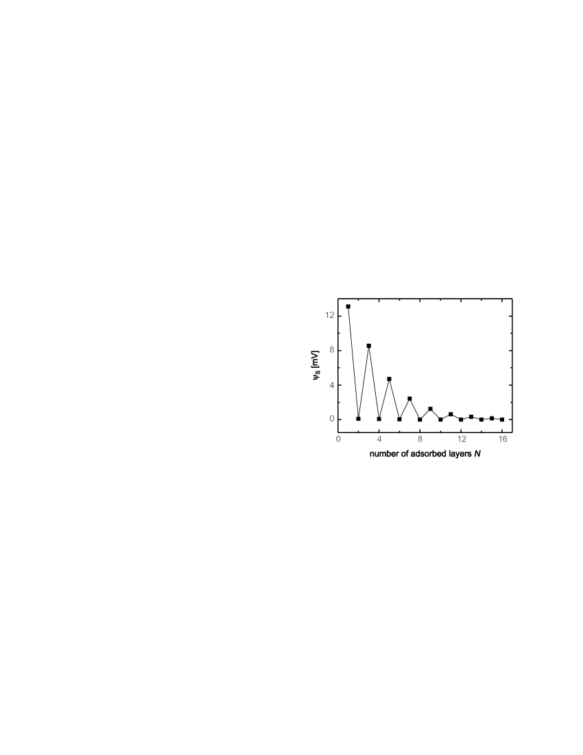
Figure 5: The potential $\psi_{\text{S}}$ was calculated within the model for the deposition from a salt concentration of 500 mM and plotted as a function of the number of adsorbed layers $N$. The solid lines are a guide to the eye. For the calculation the following parameters were assumed: $C_{\text{S}}=2\times 10^{-3}\leavevmode\nobreak\ \frac{\text{F}}{\text{m}^{2}}$, $d=2.2$ nm, $\kappa^{-1}=6.5$ nm, $\varepsilon=21$, $\sigma_{1}=-1.25\times 10^{-2}\leavevmode\nobreak\ \frac{\text{C}}{\text{m}^{2}}$ and $\sigma=2.5\times 10^{-2}\leavevmode\nobreak\ \frac{\text{C}}{\text{m}^{2}}$. In the calculation the voltage between the bulk semiconductor and the bulk electrolyte was set to $7$ mV.

Ion-partitioning between PEMs and the bulk solution

One can calculate the concentration of ions inside the PEMs from the thermodynamic equilibrium condition with the bulk solution by minimizing the total free energy density (that is free energy per unit volume) of the PEMs/bulk electrolyte system as follows.

The total free energy density consists of the free energy density of the electrical double layer outside the PEMs, ${\mathcal{F}}_{0}$, and the free energy density of the PEMs medium ${\mathcal{F}}_{\mathrm{P}}$. Within the Debye-Hückel description, the former contribution may be written as ${\mathcal{F}}_{0}={\mathcal{F}}_{0}^{\mathrm{MF}}+{\mathcal{F}}_{0}^{\mathrm{corr}}+{\mathcal{F}}_{0}^{\mathrm{self}}$ (in units of $kT$) comprising the mean-field electrostatic free energy density of the double-layer, ${\mathcal{F}}_{0}^{\mathrm{MF}}$, the Debye-Hückel correlation (or excess) free energy density, ${\mathcal{F}}_{0}^{\mathrm{corr}}$, and the self-energy density of the ions, ${\mathcal{F}}_{0}^{\mathrm{self}}$. Note that ${\mathcal{F}}_{0}^{\mathrm{corr}}$ takes into account the fact that each ion in the electrolyte is surrounded mostly by oppositely charged ions, which amounts to the standard correlation free energy expression ${\mathcal{F}}_{0}^{\mathrm{corr}}=-\kappa_{0}^{3}/12\pi$, where $\kappa_{0}=(8\pi\ell_{\mathrm{B}}^{0}c_{0})^{1/2}$ is the bulk inverse screening length with $\ell_{\mathrm{B}}^{0}=e^{2}/(4\pi\varepsilon_{\mathrm{w}}\varepsilon_{0}kT)$ being the bulk Bjerrum length . It follows that within the DH approximation, the mean-field free energy ${\mathcal{F}}_{0}^{\mathrm{MF}}$ is dominated by the entropy of the ions, which is well-approximated by that of an ideal gas of particles, i.e. ${\mathcal{F}}_{0}^{\mathrm{MF}}\simeq 2(c_{0}\ln c_{0}-c_{0})$ assuming the bulk 1-1 electrolyte concentration of $c_{0}$. Finally the self-energy contribution of ions reads ${\mathcal{F}}_{0}^{\mathrm{self}}=2c_{0}\ell_{\mathrm{B}}^{0}/2a$ (in units of $kT$).

Similar expressions may be written for the PEMs medium using the inverse screening length $\kappa=(8\pi\ell_{\mathrm{B}}c)^{1/2}$, the Bjerrum length $\ell_{\mathrm{B}}=e^{2}/(4\pi\varepsilon\varepsilon_{0}kT)$ and the ionic concentration $c$. In this case, the mean-field free energy is again approximated by that of an ideal gas since the net charge within the PEMs is assumed to be zero. One thus has ${\mathcal{F}}_{\mathrm{P}}(c)=2(c\ln c-c)-\kappa_{0}^{3}/(12\pi)+2c\ell_{\mathrm{B}}/2a$.

Thermodynamic equilibrium is imposed by minimizing ${\mathcal{F}}_{\mathrm{P}}(c)+{\mathcal{F}}_{0}(c_{0})$ with respect to the ion concentration $c$ inside the PEMs, assuming that $c+c_{0}$ is constant, which is equivalent to setting equal chemical potentials for the two media. One thus finds the ion-partitioning law $c=c_{0}\exp(-\Delta\mu/kT)$, where

$$\Delta\mu=\frac{\ell_{\mathrm{B}}}{2}\left(\frac{1}{a}-\frac{1}{\kappa^{-1}}\right)-\frac{\ell_{\mathrm{B}}^{0}}{2}\left(\frac{1}{a}-\frac{1}{\kappa_{0}^{-1}}\right).$$

The terms proportional to $1/a$ (with $a$ being the mean ion radius) are due to the self-energy (Born energy) difference of the ions in the two media, whereas the terms proportional to the Debye screening length come from the DH correlation free energy difference. Since $\kappa^{-1}$ and $\kappa_{0}^{-1}$ are typically much larger than $a$, one can neglect this latter contribution. In fact, an explicit estimate of the dielectric constant of the PEMs, $\varepsilon$, including the DH correlation free energy shows slightly larger values (up to a few percents) as compared with the results reported in the text (obtained based only on the Born energy). The difference is however within the experimental error bars.

References

- [1] Decher, G. Science 1997, 227, 1232-1237.
- [2] Bertrand, P.; Jonas, A.; Laschewsky, A.; Legras, R. Macromol. Rapid Commun. 2000, 21, 319-348.
- [3] Farhat, T.; Yassin, G.; Dubas, S. T.; Schlenoff, J. B. Langmuir 1999, 15, 6621-6623.
- [4] Sukhorukov, G. B.; Donath, E.; Lichtenfeld, H.; Knippel, E.; Knippel; M.; Budde, A.; Möhwald, H. Coll. Sufaces A 1998, 137, 253-266.
- [5] Schlenoff, J. B.; Ly, H.; Li, M. J. Am. Chem. Soc. 1998, 120, 7626-7634.
- [6] Schmitt, J.; Grünewald, T.; Decher, G.; Pershan, P. S.; Kjaer, K.; Lösche, M. Macromolecules 1993, 26 7058-7063.
- [7] Lösche, M.; Schmitt, J.; Decher, G.; Bouwman, W. G.; Kjaer, K. Macromolecules 198, 31, 8893-8906.
- [8] von Klitzing, R.; Möhwald, H. Langmuir 1995, 11, 3554-3559.
- [9] Schollmeyer, H.; Daillant, J.; Guenoun, P.; von Klitzing, R. unpublished results.
- [10] Slevin, C. J.; Malkia, A.; Liljeroth, P.; Toiminen, M.; Kontturi, K. Langmuir 2003, 19, 1287-1294.
- [11] Pouthas, F.; Gentil, C.; Cote, D.; Zeck, G.; Straub, B.; Bockelmann, U. Physical Review E 2004, 70, 031906.
- [12] Fritz, J.; Cooper, E. B.; Gaudet, S.; Sorger, P. K.; Manalis, S. R. PNAS 2002, 99 (22), 14142-14146.
- [13] Uslu, F.; Ingebrandt, S.; Mayer, D.; Böcker-Meffert, S.; Odenthal, M.; Offenhäusser, A. Biosensors and Bioelectronics 2004, 19, 1724-1731.
- [14] Nikolaides, M. G.; Rauschenbach, S.; Luber, S.; Buchholz, K.; Tornow, M.; Abstreiter, G.; Bausch, A. B. ChemPhysChem 2003, 4, 1104-1106.
- [15] Nikolaides, M. G.; Rauschenbach, S.; Bausch, A. B. Journal of Applied Physics 2004, 95 (7), 3811-3815.
- [16] Siu, W. M.; Cobbold, R. S. C. IEEE Transactions On Electron Devices 1979, ED-26 (11), 1805-1815.
- [17] Netz, R. R.; Joanny, J.-F. Macromolecules 1999, 32, 9013-9025.
- [18] Reich, C.; Hochrein, M.; Krause, B.; Nickel, B. Review of Scientific Instruments 2005, 76, 095103.
- [19] Israelachvili, J. N. Intermolecular and surface forces; Academic Press: London, 1991.
- [20] Netz, R. R. European Physical Journal E 2000, 3, 131-141.
- [21] Tedeschi, C.; Möhwald, H.; Kirstein, S. J. Am. Chem. Soc. 2001, 123, 954-960.
- [22] Durstock, M. F.; Rubner, M. F. Langmuir 2001, 17, 7865-7872.
- [23] Steitz, R.; Leiner, V.; Siebrecht, R.; von Klitzing, R. Coll. Sufaces A 2000, 163, 63-70.
- [24] Wong, J. E.; Rehfeldt, F.; Haenni, P.; Tanaka, M.; von Klitzing, R. Macromolecules 2004, 37, 7285-7289.
- [25] Carriere, D.; Krastev, R.; Schönhoff, M. Langmuir 2004, 20, 11465-11472.
- [26] Schwarz, B.; Schönhoff, M. Langmuir 2002, 18, 2964-2966.