Walks on weighted networks

Abstract

We investigate the dynamics of random walks on weighted networks. Assuming that the edge’s weight and the node’s strength are used as local information by a random walker, we study two kinds of walks, weight-dependent walk and strength-dependent walk. Exact expressions for stationary distribution and average return time are derived and confirmed by computer simulations. We calculate the distribution of average return time and the mean-square displacement for two walks on the BBV networks, and find that a weight-dependent walker can arrive at a new territory more easily than a strength-dependent one.

There has been a long history of studying random walks to model various dynamics in physical, biological, social, and economic systems Spitzer . A large body of theoretical results are available for random walks performed on regular lattices and on the Cayley (or regular) trees Barber ; Hughes , which are defined to be trees with homogeneous vertex degree. However, it has been suggested recently that more complex networks as opposed to regular graphs and conventional random graphs Erdos are concerned to real worlds. Particularly, important classes of random graphs such as small-world networks Watts and scale-free networks Barabasi were proposed and have been examined in the last several years. These networks share some important properties with real networks, such as the clustering property, short average path length, and the power-law of the vertex degree distributions. They have been applied to the analysis of various social, engineering, and biological networks including epidemic spreading, percolation, and synchronization, et al Watts_1 ; Dorogovtsev ; Newman ; Strogatz .

Recently, there have been several studies of random walks on small-world networks Pandit ; Lahtinen ; Almaas ; Parris and on scale-free networks Adamic ; Noh ; Gallos ; Yang . Most of studies of random walks focus on unweighted networks, however, the study of the dynamics of random walks on weighted networks is missing while most of real networks are weighted characterized by capacities or strengths instead of a binary state (present or absent) Yook ; Zheng ; Park ; Barrat ; Wu ; Guimera . In the weighted networks, a weight $w_{ij}$ is assigned to the edge connecting the vertices $i$ and $j$, and the strength of the vertex $i$ can be defined as

$$s_{i}=\sum_{j\in\nu(i)}w_{ij},$$ (1)

where the sum runs over the set $\nu(i)$ of neighbors of $i$. The strength of a node integrates the information about its connectivity and the weights of its links.

In this paper we study the dynamics of random walk processes on weighted networks by means of BBV model Barrat . The model starts from an initial number of completely connected vertices $m_{0}$ with a same assigned weight $w_{0}$ to each link. At each subsequent time step, addition of a new vertex $n$ with $m_{0}$ edges and corresponding modification in weights are implemented by the following two rules: (i) The new vertex $n$ is attached at random to a previously existing vertex $i$ with the probability that is proportional to the strength of node $i$, $s_{i}/\sum_{j}s_{j}$, implying new vertices connect more likely to vertices handling larger weights. (ii) The additional induced increase $\delta$ in strength $s_{i}$ of the $i$th vertex is distributed among its nearest neighbors $j\in{\cal V}(i)$ according to the rule

$$w_{ij}\rightarrow w_{ij}+\delta\frac{w_{ij}}{s_{i}},$$ (2)

which considers that the establishment of a new edge of weight $w_{0}$ with the vertex $i$ induces a total increase of traffic $\delta$ that is proportionally distributed among the edges departing from the vertex according to their weights. The BBV model suggests two ingredients of self-organization of weighted networks, strength preferential attachment and weight evolving dynamics Barrat . Considering an arbitrary finite weighted network which consists of nodes $i=1,\ldots,N$ and links connecting them. The connectivity is represented by the adjacency matrix A whose element $a_{ij}=1$ if there is a link from $i$ to $j$, and $a_{ij}=0$ otherwise. The information of edges weight is represented by matrix W whose element $w_{ij}$ is the weight of the edge between $i$ and $j$. We restrict ourselves to an undirected network $a_{ij}=a_{ji}$ and symmetrical edge’s weight $w_{ij}=w_{ji}$.

Assuming that edge’s weight and node’s strength are used as local information by a random walker, we define two kinds of walks, weight-dependent walk and strength-dependent walk. For weight-dependent walk, a walker chooses one of its nearest neighbors with the probability that is proportional to the weight of edge linked them. The transition probability from node $i$ to its neighbor $j$ is

$$p_{i\rightarrow j}^{w}=\frac{w_{ij}}{s_{i}}.$$ (3)

When time becomes infinite, one can find the walker staying at node $i$ with the probability $P_{i}^{w}$, which is defined as the stationary distribution. Following the ideas developed by Noh and Rieger Noh , we can write

$$P_{i}^{w}=\frac{s_{i}}{\sum_{j}s_{j}},$$ (4)

namely, the larger strength a node has, the more often it will be visited by a random walker.

For strength-dependent walk, a walker at node $i$ at time $t$ selects one of its neighbors with the probability which is proportional to the selected node’s strength to which it hops at time $t+1$. The transition probability from node $i$ to its neighbor $j$ is

$$P_{i\rightarrow j}^{s}=\frac{s_{j}a_{ij}}{s_{i}^{{}^{\prime}}},$$ (5)

where $s_{i}^{{}^{\prime}}=\sum_{l\in\nu(i)}s_{l}$ and $\nu(i)$ denotes the set of all neighboring vertices of node $i$. Supposing that a walker starts at node $i$, and the probability that the walker at node $k$ after $t$ time steps denoted by $P_{ik}^{s}(t)$, then the master equation for the probability $P_{i\rightarrow j}^{s}$ to find the walker at node $j$ at time $t+1$ is

$$P_{i\rightarrow j}^{s}(t+1)=\sum_{k}\frac{s_{j}a_{kj}}{s_{k}^{{}^{\prime}}}P_{ik}^{s}(t).$$ (6)

An explicit expression for the transition probability $P_{i\rightarrow j}^{s}(t)$ to go from node $i$ to node $j$ in $t$ steps follows by iterating Eq. (6)

$$P_{i\rightarrow j}^{s}(t)=\sum_{j_{1},\ldots,j_{t-1}}\frac{s_{j_{1}}a_{ij_{1}}}{s_{i}^{{}^{\prime}}}\cdot\frac{s_{j_{2}}a_{j_{1}j_{2}}}{s_{j_{1}}^{{}^{\prime}}}\cdots\frac{s_{j}a_{j_{t-1}j}}{s_{j_{t-1}}^{{}^{\prime}}}.$$ (7)

Comparing the expressions for $P_{i\rightarrow j}^{s}(t)$ and $P_{j\rightarrow i}^{s}(t)$, we get

$$s_{i}s_{i}^{{}^{\prime}}P_{i\rightarrow j}^{s}(t)=s_{j}s_{j}^{{}^{\prime}}P_{j\rightarrow i}^{s}(t).$$ (8)

This is a direct consequence of the undirectedness of the network. We can also define the probability $P^{s}_{i}$ as the stationary distribution when the evolving time becomes infinite. Eq. (8) implies that $s_{i}s_{i}^{{}^{\prime}}P_{j}^{s}=s_{j}s_{j}^{{}^{\prime}}P_{i}^{s}$, and therefore one can obtain Noh

$$P_{i}^{s}=\frac{s_{i}s_{i}^{{}^{\prime}}}{\sum_{l}s_{l}s_{l}^{{}^{\prime}}}.$$ (9)

Now we discuss the stationary distribution for edges, i.e., the probability that an edge is chosen by the walker to follow as the evolving time becomes infinite. In unweighted networks, all edges are equal and a random walker will choose one of its neighboring edges at the same probability. So each edge in the network has the same probability to be chosen by the walker when $t\rightarrow\infty$ for weight-dependent walk. In weighted networks, however, the walker will choose an edge according to the weight of it or the strength of the node connected by it. Then the relation between the stationary distribution for edges $P_{e_{ij}}$ and the stationary distribution for nodes $P_{i}$ can be written as

$$P_{e_{ij}}=P_{i}P_{i\rightarrow j}+P_{j}P_{j\rightarrow i},$$ (10)

where $P_{i\rightarrow j}$ is the transition probability from node i to node j. For weight-dependent walk, substituting Eqs. (3) and (4) into Eq. (10), we obtain the stationary distribution for edges

$$P_{e_{ij}}^{w}=\frac{2w_{ij}}{\sum_{k,l}w_{kl}}.$$ (11)

For strength-dependent walk, substituting Eqs. (5) and (9) into Eq. (10), we obtain the stationary distribution for edges

$$P^{s}_{e_{ij}}=\frac{2s_{i}s_{j}}{\sum_{k,l}s_{k}s_{l}a_{kl}}.$$ (12)

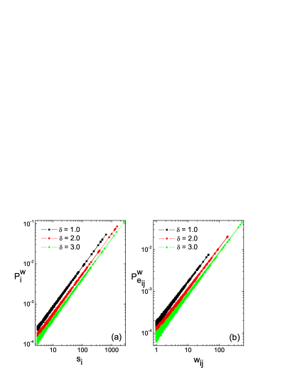
Figure 1: Log-log plots of $P_{i}^{w}$ vs. $s_{i}$ (a) and $P^{w}_{e_{ij}}$ vs. $w_{ij}$ (b) in the BBV network with $N=1000$, $m_{0}=3$ and different values of $\delta$. Slopes of all the curves are equal to $0.9999\pm 0.0006$. The data were obtained after walking $10^{8}$ steps on the network.

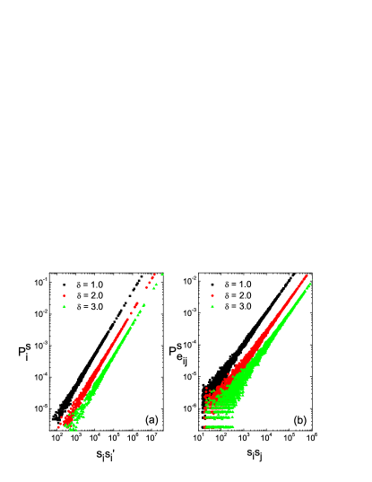
Figure 2: Log-log plots of $P_{i}^{s}$ vs. $s_{i}s_{i}^{{}^{\prime}}$ (a) and $P^{s}_{e_{ij}}$ vs. $s_{i}s_{j}$ (b) in the BBV network with $N=1000$, $m_{0}=3$ and different values of $\delta$. Slopes of all the curves are equal to $1.018\pm 0.003$. The data were obtained after walking $10^{8}$ steps on the network.

In Fig. 1 we plot $P_{i}^{w}$ vs. $s_{i}$ (Fig. 1(a)) and $P^{w}_{e_{ij}}$ vs. $w_{ij}$ (Fig. 1(b)) in log-log scale in the BBV network. The power-law property of Eqs. (4) and (11) is presented in excellent agreement with the numerical results. In Fig. 2 we show the log-log plots of $P_{i}^{s}$ vs. $s_{i}s_{i}^{{}^{\prime}}$ (Fig. 2(a)) and $P^{s}_{e_{ij}}$ vs. $s_{i}s_{j}$ (Fig. 2(b)) in the BBV model. The numerical results are also in good agreement with Eqs. (9) and (12).

Next we study average return time which is the average time spent by a walker to return to its origin. From its definition, we can easily obtain that the average return time is equal to the reciprocal of the stationary distribution. The average return time for node $i$ is

$$\langle T_{ii}^{w}\rangle=\frac{1}{P_{i}^{w}}=\frac{\sum_{j}{s_{j}}}{s_{i}},$$ (13)

for weight-dependent walk and

$$\langle T^{s}_{ii}\rangle=\frac{1}{P_{i}^{s}}=\frac{\sum_{j}s_{j}s_{j}^{{}^{\prime}}}{s_{i}s_{i}^{{}^{\prime}}}.$$ (14)

for strength-dependent walk, respectively.

Using the same methods, the average return time for edge $e_{ij}$ can also be obtained

$$\langle T^{w}_{e_{ij}}\rangle=\frac{\sum_{k,l}w_{kl}}{2w_{ij}},$$ (15)

for weight-dependent walk and

$$\langle T^{s}_{e_{ij}}\rangle=\frac{\sum_{k,l}s_{k}s_{l}a_{kl}}{2s_{i}s_{j}}.$$ (16)

for strength-dependent walk, respectively.

Figure 3: Numerical results for the average return time of node for the two different walks , weight-dependent walk (a) and strength-dependent walk (b), on the BBV network with $N=1000$, $m_{0}=3$ and $\delta=1.0$. The data were averaged on 1000 networks and obtained after walking $10^{6}$ steps in each network.

In Fig. 3 we show the log-log plots of $\langle T_{ii}^{w}\rangle$ vs. $s(i)$ and $\langle T_{ii}^{s}\rangle$ vs. $s(i)$ in the BBV networks. The slope of the curve in Fig. 3(a) is $-0.9903\pm 0.0007$, consistent with Eq. (13). The BBV networks have two properties in Barrat : (i) node’s strength is proportional to node’s degree, $s_{i}\sim k_{i}$; (ii) the average nearest neighbor degree is $k_{nn}(k)\sim k^{-2+1/\beta}$ with $\beta=(2\delta+1)/(2\delta+2)$. Considering these two ingredients, one can observe that $s_{i}s_{i}^{{}^{\prime}}\sim s_{i}^{1/\beta}$, and obtain $\langle T_{ii}^{s}\rangle\sim s^{-1/\beta}_{i}$. Fig. 3(b) gives that $-1/\beta=-1.355\pm 0.006$ which agrees with the theoretical value $-1/\beta=-(2\delta+2)/(2\delta+1)=-4/3$. In Fig. 3 the slope of the curve for strength-dependent walk is steeper than that for weight-dependent walk, giving rise to a broader distribution of average return time for strength-dependent walk. In order to confirm this point, we derive the expression for the distribution of average return time. In BBV network, we know that the strength distribution behaves as $P(S)\sim S^{-\gamma}$, where $\gamma=(3+4\delta)/(1+2\delta)$ Barrat . According to the above analysis, we can obtain that the distribution of average return time is $P(T^{w})\sim(T^{w})^{-1/(1+\delta)}$ for the weight-dependent walk, and $P(T^{s})\sim 1.0$ for the strength-dependent case. Thus, we can see, for those nodes with large strength the strength-dependent walker spends more time in visiting them than that the weight-dependent walker does. This point can be reflected by the difference of the mean-square displacement for two walks which is shown in the following.

The mean-square displacement $\langle R^{2}\rangle$ is a measure of the distance $R$ covered by a typical random walker after performing $t$ steps Almaas ; Gallos . To calculate this quantity we first, at each time step, find the minimal distance from the current position of the walker to the origin (i.e., the smallest number of steps needed for the walker to reach the origin ) using a breadth-first search method. Then we allow the walker to move through the network until $<R^{2}>$ has saturated. Finally, we average over different initial positions of the walker and realizations of the network. Fig. 4 shows the results of $\langle R^{2}\rangle$ as a function of time $t$. We note that $\langle R^{2}\rangle$ equilibrates after a few steps to a constant displacement value. This is a simple manifestation of the very small diameter of the BBV network. Note also that the value of plateau is higher for weight-dependent walk than that for strength-dependent walk. That is, a strength-dependent walker spends more time in visiting these nodes with large strength or large degree, i.e. a weight-dependent walker can arrive at a new territory more easily than a strength-dependent walker.

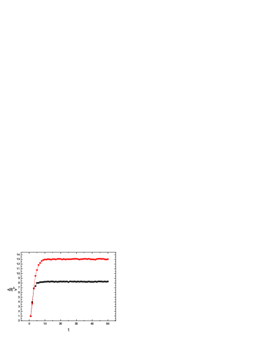
Figure 4: Mean-square displacement $\langle R^{2}\rangle$ as a function of time $t$ for two kinds of walks, weight-dependent walk (closed circles) and strength-dependent walk (closed squares), on the BBV network with $N=10^{5}$, $m_{0}=3$, and $\delta=1.0$. All the plots were averaged over $1000$ different initial positions of the walker and $20$ realizations of the network.

In summary, we have studied two different types of walks on weighted networks, weight-dependent walk and strength-dependent walk. We derived exact expressions for the stationary distribution and the average return time for the two walk processes, and confirmed them by simulations on BBV networks. Then we analysed the distribution of average time for two walks and found that it is broader for dependent-strength walk than that for dependent-weight walk on the BBV network. Finally we computed the mean-square displacement $\langle R^{2}\rangle$. For both walks, $\langle R^{2}\rangle$ was found to reach the saturation after a few time steps which is a result of the very small diameter of the underlying graph. Furthermore, the difference of average-square displacement for two walks implies that a weight-dependent walker can arrive at a new territory more easily than a strength-dependent walker on the BBV network.

References

- (1) F. Spitzer, Principles of Random Walk, 2nd ed. (Springer- Verlag, New York, 1976).
- (2) M.N. Barber and B.W. Ninham, Random and Restricted Walks (Gordon and Breach, New York, 1970).
- (3) R.D. Hughes, Random Walks and Random Environments (Clarendon, Oxford, 1996), Vols. 1 and 2.
- (4) P. Erdös and A. Rényi, Publ. Math. 6, 290 (1959); Publ. Math. Inst. Hung. Acad. Sci. 5, 17 (1960).
- (5) D.J. Watts and S.H. Strogatz, Nature 393, 440 (1998).
- (6) A.-L. Barabási and R. Albert, Science 286, 509 (1999); A.-L. Barabási, R. Albert, and H. Jeong, Physica A 272, 173 (1999).
- (7) D.J. Watts, Small Worlds: The Dynamics of Networks Between Order and Randomness (Princeton University Press, New Jersey, 1999).
- (8) S.N. Dorogovtsev and J.F.F. Mendes, Adv. Phys. 51, 1079 (2002).
- (9) M.E.J. Newman, SIAM Rev. 45, 167 (2003).
- (10) S.H. Strogatz, Nature (London) 410, 268 (2001).
- (11) S.A. Pandit and R.E. Amritkar, Phys. Rev. E 63, 041104 (2001).
- (12) J. Lahtinen, J. Kertész, and K. Kaski, Phys. Rev. E 64, 057105 (2001).
- (13) E. Almaas, R.V. Kulkarni, and D. Stroud, Phys. Rev. E 68, 056105 (2003).
- (14) P.E. Parris and V.M. kenkre, Phys. Rev. E 72, 056119 (2005).
- (15) L.A. Adamic, R.M. Lukose, A.R. Puniyani, and B.A. Huberman, Phys. Rev. E 64, 046135 (2001).
- (16) J.D. Noh and H. Rieger, Phys. Rev. Lett 92, 118701 (2004); Phys. Rev. E 69, 036111 (2004); cond-mat/0509564.
- (17) L.K. Gallos, Phys. Rev. E 70, 046116 (2004).
- (18) S.-J. Yang, Phys. Rev. E 71, 016107 (2005).
- (19) S.H. Yook, H. Jeong, and A.-L. Barabási, and Y. Tu, Phys. Rev. Lett. 86, 5835 (2001).
- (20) D. Zheng, S. Trimper, B. Zheng, and P.M. Hui, Phys. Rev. E 67, 040102(R) (2003).
- (21) K. Park, Y.-C. Lai, and N. Ye, Phys. Rev. E 70, 026109 (2004).
- (22) A. Barrat, M. Barthélemy, R. Pastor-Satorras, and A. Vespignai, Proc. Natl. Acad. Sci. USA 101, 3747 (2004); A. Barrat, M. Barthélemy, and A. Vespignani, Phys. Rev. Lett. 92, 228701 (2004); Phys. Rev. E 70, 066149 (2004); A. Barrat and R. Pastor-Satorras, Phys. Rev. E 71, 036127 (2005).
- (23) Z.-X. Wu, X.-J. Xu, and Y.-H. Wang, Phys. Rev. E 71, 066124 (2005).
- (24) R. Guimera, S. Mossa, A. Turtschi, and L.A.N. Amaral, Proc. Natl. Acad. Sci. USA 102, 7794 (2005).