Low-Temperature Quasi-Equilibrium States in the Hydrogen Atom

Abstract

The dynamics of the approach to equilibrium of the hydrogen atom is investigated numerically through a Monte Carlo procedure. We show that, before approaching ionization, the hydrogen atom may live in a quasi-equilibrium state, characterized by aging, whose duration increases exponentially as the temperatures decreases. By analyzing the quasi-equilibrium state, we compute averages of physical quantities for the hydrogen atom. We have introduced an analytic approach that fits satisfactorily the numerical estimates for low temperatures. Although the present analysis is expected to hold for energies typically up to $6\%$ of the ionization energy, it works well for temperatures as high as $10^{4}$ K.

Keywords: Hydrogen Atom; Metastability; Aging; Thermodynamic Properties.

1.  Introduction

Obtaining equilibrium properties for the hydrogen atom in free space, through standard Boltzmann-Gibbs (BG) statistical mechanics, is troublesome, since the partition function diverges for any finite temperature. This occurs mostly in systems of composite particles, which are characterized by upper bounds, preceded by a quasi-continuum of energy levels, in their energy spectra. Each of the levels in the quasi-continuum yields a small contribution for the partition function; the divergence arises since there are, in principle, an infinite number of such levels. Essentially, this reflects the fact that composite particles always ionize at any finite temperature. Due to these difficulties, such systems are never discussed in standard statistical-mechanics textbooks (for an exception of this, see Ref. fowler ).

However, the presence of long-living nonionized hydrogen atoms in galaxy peripheries and in intergalactic media, at low temperatures, is undeniable. Certainly, their density must be very low in such a media, in order to avoid combination (${\rm H}+{\rm H}\rightarrow{\rm H}_{2}$), and they should spend a long time in their nonionized state, before reaching ionization. These long-living quasi-equlibrium states represent the main point we explore, on theoretical grounds, in the present work.

The specific heat of the hydrogen atom has been calculated recently liacir through the generalized statistical-mechanics formalism tsallisbjp ; abeokamoto ; grigolini that emerged from Tsallis’s generalization of the BG entropy tsallis88 . Within this approach, the specific heat was computed for certain values of the entropic index $q<1$ (notice that $q=1$ corresponds to the standard BG formalism). Even within such a formalism, the hydrogen-atom specific heat presents several anomalies, like divergences, cusps, and discontinuities in its derivative liacir .

Herein, we choose a different approach for analyzing this problem, as described next.

(i) We investigate the dynamical behavior of the hydrogen atom by applying a standard Monte Carlo method, in which the probability for jumping between states is based on the BG weight. As expected, for any finite temperature, the simulation always carries the system towards ionization, after some time. However, it is shown that the system may live in a quasi-equilibrium state, characterized by a slowly varying value of the average energy, before approaching its maximum-energy state. The time that the system remains on such a quasi-equilibrium state increases for lowering temperatures.

(ii) We propose a modified dynamics that prevents the system from reaching ionization and whose results coincide, during some time (essentially when the system lies in its low-temperature quasi-equilibrium state), with those of the standard dynamics. Therefore, for low temperatures, depending on time scale of interest, the modified dynamics may reflect the correct dynamical behavior of the system. The advantage of the modified dynamics is that its corresponding partition function, associated to the statistical weight that generated it, is finite and may be calculated exactly.

(iii) Since the quasi-equilibrium state may present a long duration for low temperatures, herein we will consider it as an effective equilibrium. Therefore, if the results obtained from the standard and modified dynamics coincide within such a quasi-equilibrium state, one may use the later formalism in such a way to compute thermodynamic properties.

(iv) We introduce a modified regularized partition function, by extracting the divergence of the BG partition function, for a hydrogen atom, and compare the corresponding internal energy and specific heat with the results obtained from the numerical simulations.

(v) Obviously, the procedures described above may work as good approximations for low energies, but should fail for increasing energies. Since our energies are always measured with respect to the corresponding ionization energy, we show that our approximations work well for energies that correspond to temperatures much higher than room temperature.

In the next section we investigate the dynamical behavior of the hydrogen atom within a standard Monte Carlo framework. In section 3 we introduce a modified dynamics and apply it for the hydrogen atom. In section 4 we calculate a regularized partition function, related to the modified dynamics introduced in section 3, and compute some associated thermodynamic quantities for the hydrogen atom. In section 5 we propose two possible physical realizations for the quasi-equilibrium states presented herein. Finally, in section 6 we present our conclusions.

2.  The Hydrogen Atom within a Standard Monte Carlo Procedure

Let us consider a hydrogen atom with its well-known energy spectrum (see, e.g., ref. cohen , page 790),

$$E_{n}=R\left(1-{1\over n^{2}}\right)\qquad(n=1,2,\cdots),$$

where $R$ is the Rydberg constant [$R=13.6058$ eV, or $R=2.18\times 10^{-18}$ J, which corresponds to a temperature $(R/k_{B})=1.579\times 10^{5}$ K], and we have chosen the ground state to have zero energy. As $n$ increases, one has a quasi-continuum of energy levels, and in the limit $n\rightarrow\infty$ the atom ionizes (with an ionization energy $E^{*}=R$), in such a way that the gap separating the ground-state and ionization energies is $R$. A transition between the ground state and the first-excited state costs most of the energy of the gap, i.e., $3R/4$, whereas all further jumps occur in the range $R/4$. Therefore, for low temperatures, the hydrogen atom is expected to remain a long time in the lowest-energy states (mostly in the ground state). However, as the quantum number $n$ increases, the energy cost for jumps between nearest-neighbor levels decreases. Therefore, once the system has reached a state characterized by a large quantum number $n$, transitions to higher-energy levels cost very little energy, in such a way that after a long time, the hydrogen atom will ionize. The ionization will always occur for any finite temperature; one of the questions we address in the present work is how long does the system remains in the quasi-equilibrium state (characterized by an average energy close to the ground-state energy).

It is important to remind that the above energy spectrum is degenerate (see, e.g., ref. cohen , page 798), in such a way that a given energy level $E_{n}$ presents a total degeneracy $g_{n}=n^{2}$. Therefore, a precise analysis of this problem should take into account the degeneracy of the energy levels, as well as of the spins. However, in the present investigation, only the lowest energy levels will contribute most significantly, in such a way that the effects of the degeneracy will not change qualitatively our results. Consequently, we will consider herein, $g_{n}=1\ (\forall n)$, for simplicity.

We have investigated the dynamical behavior of the hydrogen atom through a Monte Carlo procedure garrod . The probabilities $P(n+1\rightarrow n)$ and $P(n\rightarrow n+1)$, for transitions between the states characterized by quantum numbers $n$ and $n+1$, satisfying the detailed-balance condition and constructed by using the standard BG weight, are given by

$$P(n+1\rightarrow n)=c~{},\qquad P(n\rightarrow n+1)=c\ \exp[-\beta(E_{n+1}-E_{n})]~{},$$

where $\beta=(k_{B}T)^{-1}$ and $c$ is an arbitrary constant ($0<c\leq 1/2$). In order to implement the dynamical evolution, a uniform random number $z$ ($z\in[0,1]$) must be generated at each Monte Carlo step (which will be adopted as our unit of time). For a system in a state characterized by the quantum number $n$ at time $t$, transitions between states are performed (or not), depending on the value of $z(t)$, according to the following rules:

(i) If $z(t)\leq P(n\rightarrow n+1)$, perform the jump $n\rightarrow n+1$;

(ii) If $P(n\rightarrow n+1)<z(t)\leq[P(n\rightarrow n+1)+P(n\rightarrow n-1)]$, perform the jump $n\rightarrow n-1$;

(iii) Else, remain on level $n$.

One may easily see that the constant $c$ is proportional to the probability for no jumps [rule (iii)]. In the following results we have used $c=1/2$, although we have verified that other choices for this constant ($0<c<1/2$) did not change qualitatively our results. Below, $\langle\ \rangle$ correspond to averages over $N_{s}$ distinct samples, i.e., different sequences of random numbers. We have considered two distinct initial conditions in our simulations, which will be reffered to, herein, as conditions 1 and 2, corresponding to all samples starting with the quantum number $n=1$ (condition 1), and all samples starting with $n=2$ (condition 2). Although, in some cases, the results obtained by using these two initial conditions seem to be different, they approach each other in the limit $N_{s}\rightarrow\infty$ (except, of course, in the transient regimes, before reaching the quasi-equilibrium state).

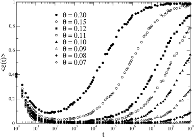
Figure 1: The time evolution of the average dimensionless energy (energy in units of the Rydberg constant), for the hydrogen atom, is represented for several relative temperatures ($\theta=k_{B}T/R$). Time is measured in Monte Carlo steps.

In Fig. 1 we present the time evolution of the average dimensionless energy, $\langle\varepsilon(t)\rangle$ [$\varepsilon_{n}=E_{n}/R$], for several values of the relative-temperature variable, $\theta=(k_{B}T)/R$, i.e., the ratio of the temperature with respect to the Rydberg constant. Our simulations were carried up to a maximum time $t_{\rm max}=10^{9}$, whereas for the averages we have considered $N_{s}=2000$ samples with the initial condition 2. Our plots exhibit a general tendency for increasing the average energy, towards the ionization energy, after some time. This reflects the fact that the hydrogen atom always ionize for any finite temperature. However, the interesting effect noticed herein is the presence of a quasi-equilibrium state, characterized by a slowly varying average energy, before the approach to ionization. Such a quasi-equilibrium state may present a long duration for low values of $\theta$, as shown in Fig. 1.

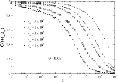
Figure 2: The two-time autocorrelation function $C(t+t_{w},t_{w})$, for the hydrogen atom, is represented against time, for a given value of the relative temperature and several waiting times $t_{w}$. Time is measured in Monte Carlo steps.

It is important to notice that such a state presents quite nontrivial behavior, e.g. it is characterized by aging, as observed on a similar system neto04 . In order to see this effect, let us define the two-time autocorrelation function cugliandolo ,

$$C(t+t_{w},t_{w})={\langle\varepsilon(t+t_{w})\varepsilon(t_{w})\rangle-\langle\varepsilon(t+t_{w})\rangle\langle\varepsilon(t_{w})\rangle\over\sigma(t+t_{w})\sigma(t_{w})},$$

where $t_{w}$ represents the well-known “waiting time”, and

$$\sigma(t)=\left[\langle(\varepsilon(t))^{2}\rangle-\langle\varepsilon(t)\rangle^{2}\right]^{1/2}.$$

In Fig. 2 we exhibit such a correlation function for a value of the relative temperature $\theta=0.08$ and several waiting times. The initial conditions are the same as in Fig. 1, but now, the averages that appear in Eqs. (3) were taken over $N_{s}=350000$ samples. The waiting times considered were chosen in such a way to ensure that the correlation function $C(t+t_{w},t_{w})$ was evaluated with the system on the quasi-equilibrium state (which is typically inside the time range $10^{2}\rightarrow 10^{8}$, as shown in Fig. 1). Clearly, there is a dependence on the waiting time typical of the aging effect cugliandolo .

3.  The Hydrogen Atom and the Modified Monte Carlo Procedure

We have also considered the evolution of the system under a modified dynamics, which satisfies detailed balance, but prevents the approach to ionization (the justification for that will become clear later on). The jumping probabilities are given by

$$P(n+1\rightarrow n)=c~{},\qquad P(n\rightarrow n+1)=c\ {\exp(-\beta E_{n+1})-\exp(-\beta R)\over\exp(-\beta E_{n})-\exp(-\beta R)}~{}.$$

In Fig. 3 we compare the results for the time evolution of the average dimensionless energy obtained by using the standard dynamics [Eq. (2)] with those obtained through the modified dynamics [Eq. (4)], for typical values of the relative temperature. The conditions for the simulations in Fig. 3 are the same as those of Fig. 1, which correspond to $t_{\rm max}=10^{9}$ and $N_{s}=2000$ (initial condition 2). One observes that the agreement between the two dynamical procedures persists during a given time (essentially within the quasi-equilibrium state), that increases for lowering values of the temperature. Within the modified dynamics, which was constructed in such a way to avoid the system from reaching ionization, the system remains on a quasi-equilibrium state forever.

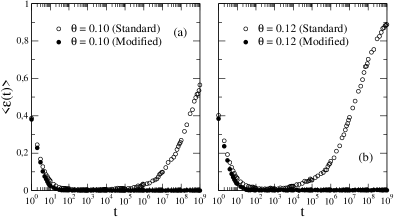
Figure 3: The time evolution (in Monte Carlo steps) of the average dimensionless energy (energy in units of the Rydberg constant), for the hydrogen atom, is represented for two relative temperatures ($\theta=k_{B}T/R$), in the case of the standard (empty symbols) and modified dynamics (full symbols).

Let us define the duration of the quasi-equilibrium state, $t_{\rm MS}(\theta)$, as the time during which the system remains on such a state, within the standard dynamics, by keeping the absolute value of the difference between the average dimensionless energies computed from the standard and modified dynamics less than a given value $\delta$. Although the choice of $\delta$ may be arbitrary, one expects the corresponding law followed by $t_{\rm MS}(\theta)$ to be independent of this particular choice. In the present analysis we estimated $t_{\rm MS}(\theta)$ by considering several values of $\theta$ from $0.08$ up to $0.12$, by imposing that $\delta$ does not exceed $0.05$. Our data fit well the exponential law,

$$t_{\rm MS}(\theta)\sim\exp(b/\theta)=\exp[bR/(k_{B}T)]\qquad(b=1.95\pm 0.06),$$

which implies $t_{\rm MS}(\theta)\rightarrow\infty$ when $T\rightarrow 0$. Essentially, the duration of the quasi-equilibrium state follows an Arrenhius law, typical of the Kramers’ escape problem in chemical reactions kramers ; hanggi , where the system may remain for a long time in a quasi-stationary state, before overcoming the potential barrier associated with the reaction. To our knowledge, this is the first time that such a behavior has been associated with the dynamics of the hydrogen atom.

Therefore, for very low temperatures and depending on time scale of interest, the modified dynamics may reflect the correct dynamical behavior of the system. The advantage of the modified approach is that the corresponding partition function, associated to the statistical weight that generated Eq. (4), is finite – contrary to the one associated with the standard dynamics – and may be calculated exactly. This will be done in the next section.

4.  The Regularized Partition Function and Associated Thermodynamic Functions

In the present section we shall calculate the partition function defined through the statistical weight related to the modified dynamics, introduced above. Let us address this point by considering in detail the divergence of the partition function associated with the energy spectrum of Eq. (1),

$$Z=\sum_{n=1}^{\infty}{\rm exp}(-\beta E_{n})={\rm exp}(-\beta R)\sum_{n=1}^{\infty}{\rm exp}[\beta R/(n^{2})]~{}.$$

The equation above may still be written as

$$Z={\rm exp}(-\beta R)\ \lim_{n^{*}\rightarrow\infty}\ \sum_{n=1}^{n^{*}}{\rm exp}[\beta R/(n^{2})]~{},$$

where $n^{*}$ is an appropriated cutoff in the quantum number, that will be taken to infinite later on. One has that

$${\rm exp}(\beta R)Z = \lim_{n^{*}\rightarrow\infty}\ \sum_{n=1}^{n^{*}}\sum_{m=0}^{\infty}{(\beta R)^{m}\over m!}{1\over n^{2m}}=\lim_{n^{*}\rightarrow\infty}\ \sum_{n=1}^{n^{*}}\left[1+\sum_{m=1}^{\infty}{(\beta R)^{m}\over m!}{1\over n^{2m}}\right]$$ (8)

$$= \lim_{n^{*}\rightarrow\infty}\ \left[n^{*}+\sum_{m=1}^{\infty}H_{n^{*},2m}\ {(\beta R)^{m}\over m!}\right]~{},$$

where $H_{n^{*},2m}=\sum_{n=1}^{n^{*}}1/(n^{2m})$ are the harmonic numbers of order $2m$ graham . The limits $n^{*}\rightarrow\infty$ of the harmonic numbers are well-defined, leading to finite coefficients, $B_{2m}=\lim_{n^{*}\rightarrow\infty}H_{n^{*},2m}$. One has that $B_{2}=\pi^{2}/6=1.64493...$, $B_{4}=\pi^{4}/90=1.08232...$, $B_{6}=\pi^{6}/945=1.01734...$, in such a way that $B_{2m}$ converges to unit for increasing values of $m$, e.g., $B_{16}=1.00002...$. Therefore, one gets

$$Z={\rm exp}(-\beta R)\left[\lim_{n^{*}\rightarrow\infty}(n^{*})+\sum_{m=1}^{\infty}B_{2m}\ {(\beta R)^{m}\over m!}\right]~{},$$

which shows a linear divergence with the quantum number. It should be stressed that the divergent contribution of the partition function comes from a single term in the sum over $m$ of Eq. (8) (term $m=0$). Let us now introduce a “modified regularized partition function”,

$$Z^{\prime}=Z-{\rm exp}(-\beta R)\lim_{n^{*}\rightarrow\infty}(n^{*})={\rm exp}(-\beta R)\sum_{m=1}^{\infty}B_{2m}\ {(\beta R)^{m}\over m!}~{},$$

which is finite. The regularized partition function defined above may be written also as

$$Z^{\prime}=\sum_{n=1}^{\infty}{\rm exp}(-\beta E_{n})-\sum_{n=1}^{\infty}{\rm exp}(-\beta R)=\sum_{n=1}^{\infty}\left[{\rm exp}(-\beta E_{n})-{\rm exp}(-\beta R)\right]~{},$$

where one identifies the statistical weight that leads to the jumping probabilities of Eq. (4).

Obviously, $Z$ and $Z^{\prime}$ are very distinct from one another (actually, the difference between them diverges). However, for low temperatures, the hydrogen atom remains for a long time in its low-energy states. Therefore, for a given low temperature, if one considers the corresponding quasi-equilibrium state as an effective equilibrium, for which the divergent term is not relevant, one may use $Z^{\prime}$ in order to calculate thermodynamic properties as approximations. Within this formalism, the quantities that would correspond to the internal energy and specific heat are given, respectively, by

$$u^{\prime}=-R\ {\partial\ln Z^{\prime}\over\partial(\beta R)} = -R\left\{-1+{\sum_{m=1}^{\infty}m(B_{2m}/m!)\ (\beta R)^{m-1}\over\sum_{m=1}^{\infty}(B_{2m}/m!)\ (\beta R)^{m}}\right\}~{},$$ (12a)

$${c^{\prime}\over k_{B}}=(\beta R)^{2}\ {\partial^{2}\ln Z^{\prime}\over\partial(\beta R)^{2}} = (\beta R)^{2}\ \left\{{\sum_{m=1}^{\infty}m(m-1)(B_{2m}/m!)\ (\beta R)^{m-2}\over\sum_{m=1}^{\infty}(B_{2m}/m!)\ (\beta R)^{m}}\right.$$ (12b)

$$- \left.{\left[\sum_{m=1}^{\infty}m(B_{2m}/m!)\ (\beta R)^{m-1}\right]^{2}\over\left[\sum_{m=1}^{\infty}(B_{2m}/m!)\ (\beta R)^{m}\right]^{2}}\right\}~{},$$

where we keep the prime notations to remind that such thermodynamic properties were calculated by using the regularized partition function $Z^{\prime}$.

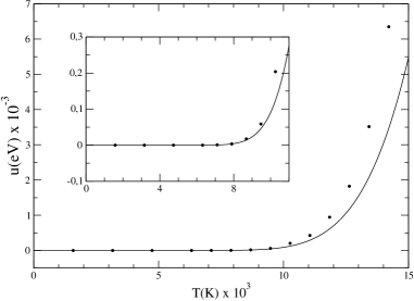
Figure 4: The internal energy of the hydrogen atom is calculated up to $T=15000$ K, by two different approximations: (i) The analytic modified regularized partition function formalism (full line); (ii) Standard Monte Carlo simulation (black dots). The inset shows an amplification of these results in the temperature range $T=0$ K $\rightarrow T=11000$ K.

In Fig. 4 we exhibit the internal energy of the hydrogen atom, as calculated from the above analytic expression [Eq. (12a)], and compare it with results of the numerical simulations. In the latter, we have computed time averages over a time interval ranging from $t_{1}=200$ up to $t_{2}=400$ Monte Carlo steps of the standard-dynamics quasi-equilibrium states, where the values at each time do already represent averages over $N_{s}=10^{6}$ samples, with the initial condition 1. Similar results may be obtained by starting the system with the initial condition 2, although a larger computational effort (i.e., higher values of $N_{s}$) may be necessary for a proper convergence towards the low-temperature quasi-equilibrium state in this case. One observes a very good agreement between the two approaches up to temperatures $10^{4}$ K. In fact, the relative discrepancy between these procedures gets larger for increasing temperatures, yielding the typical values of 0.004, for $\theta=0.05$ ($T\approx 7895$ K) and 0.282, for $\theta=0.06$ ($T\approx 9474$ K). A similar picture to the one shown in Fig. 4 holds for the specific heat of the hydrogen atom, with relative discrepancies of the same order of magnitude as those found for the internal energy. For the range of temperatures over which one finds a good agreement between the two approaches (typically from 0 K to $10^{4}$ K), the long-living low-temperature quasi-equilibrium state may be considered as an effective equilibrium state, for which the divergence of the partition function in Eq. (9) has been removed, and one may compute effective thermodynamic properties for the hydrogen atom from the regularized partition function of Eq. (10). It is important to mention that the range of temperatures over which the present regularized formalism should be applied safely for the hydrogen atom goes far beyond room temperature.

5.  Possible Physical Realizations

It seems difficult from the experimental point of view to perform measurements on a system of highly diluted nonionized hydrogen atoms, since one has to avoid the atoms from reaching ionization (which is favored at high temperatures), as well as from achieving combination, ${\rm H}+{\rm H}\rightarrow{\rm H}_{2}$ (which becomes enhanced at low temperatures). In the following discussion we propose two possible physical situations in which hydrogen atoms may be found in the above-mentioned long-living quasi-equilibrium state. In both cases, the duration of such a state is estimated in real time.

A. Gas of Hydrogen Atoms

Let us assume the viability, from the experimental point of view, for generating a gas of nonionized hydrogen atoms at low temperatures (as compared with the corresponding ionization temperature). We shall also assume that the following conditions are satisfied:

(i) The combinations, ${\rm H}+{\rm H}\rightarrow{\rm H}_{2}$, are negligible. In fact, there are experimental techniques for such a purpose, in which pairs of atoms in the so-called “spin-polarized state”, can not produce bound states silverawalraven ; silverareview ; walravenreview ;

(ii) The temperature $T$ is sufficiently low in such a way that most of the atoms that compose the gas are in the ground state;

(iii) A given hydrogen atom can only change its state through collisions with other atoms (we will assume that the linear dimension of the box enclosing the gas is much larger than its mean free path, in such a way that collisions with the walls may be neglected). An atom in its ground state may experience several collisions before excitation (actually, such an atom should undergo a collision with a sufficiently energetic atom in such a way to absorb an energy greater than $3R/4$ for a transition to occur).

Therefore, the mean time between two successive collisions, $\tau$, may be obtained from standard kinetic-theory calculations (see, e.g., ref. reif , chapter 12),

$$\tau\approx{1\over 16\sqrt{\pi}\ na^{2}}\left({m\over k_{B}T}\right)^{1/2}~{},$$

where $n$ represents the density of atoms in the gas, $m$ is the mass of the hydrogen atom, and $a$ stands for the Bohr’s radius. In the present physical system, a given atom can only change its energy through collisions with other atoms; this situation is mimicked in the Monte Carlo simulation, where at each step there is a finite probability for the occurence of a given energetic transition. In order to establish a connection between the duration of the quasi-equilibrium states of Fig. 1 (given in Monte Carlo steps) with real time, we shall propose the crude – but very suggestive – correspondence: $\tau\equiv 1$ Monte Carlo step. With this assumption, one gets that the duration (in real time) of a hydrogen atom quasi-equilibrium state, may be written as,

$$t_{\rm real}=t_{\rm MS}\ \tau\approx{1\over 16\sqrt{\pi}\ na^{2}}\left({m\over k_{B}T}\right)^{1/2}\exp[2R/(k_{B}T)]~{},$$

where we have considered the fitting parameter $b=2$ [cf. Eq. (5)]. It should be stressed that, at low temperatures, the exponential growth dominates completely, with the multiplicative factors in Eq. (14) becoming irrelevant. Therefore, the hypothesis above for the connection of Monte Carlo steps with real time may be softened in such a way that any linear relationship between a given number of successive collisions and another number of Monte Carlo steps would lead to the same exponential-growth behavior of Eq. (14).

One sees that the above duration time depends on two parameters, namely, the density of atoms and the temperature, i.e., $t_{\rm real}\equiv t_{\rm real}(n,T)$. We have estimated $t_{\rm real}(n,T)$ for the typical values $n=10^{23}{\rm atoms}/{\rm m}^{3}$ and $\theta=0.10$ ($T\approx 15797$ K), $\theta=0.05$ ($T\approx 7898$ K), $\theta=0.03$ ($T\approx 4739$ K), and $\theta=0.01$ ($T\approx 1580$ K), which yielded, respectively, the duration times, $t_{\rm real}=5.35$ seconds, $3.67\times 10^{9}$ seconds, $1.81\times 10^{21}$ seconds ($\approx 5.73\times 10^{13}$ years), and $2.52\times 10^{79}$ seconds ($\approx 8.0\times 10^{71}$ years). One notices tremendous duration times for the lowest temperatures.

It is important to remind that the above results have not taken into consideration the degeneracy of the energy spectrum, which should contribute to decrease the duration of the quasi-equilibrium states (since the degeneracy increases the number of possible transitions taking place in the Monte Carlo process). However, the enormous estimates found above, for low temperatures, should not be altered significantly due to the degeneracy of the energy spectrum.

B. Hydrogen Atoms in a Photon Bath

It is well known that long-living nonionized hydrogen atoms exist in very low concentrations and at very low temperatures (typically 3 K), in intergalactic media. These atoms are in direct contact with photons, in such a way that transitions between states occur through photon emission and absorption.

In what follows, we will present a crude estimate of a lower bound for the duration (in real time) of the above-mentioned quasi-equilibrium state for a hydrogen atom in a medium such as the intergalactic media. For that we will consider:

(i) A nonionized hydrogen atom in contact with a photon bath at a temperature $T$;

(ii) The temperature $T$ sufficiently low for the atom to be found initially in its ground state;

(iii) The velocity of the atom negligible with respect to the velocity of light.

Let us define $t_{1\rightarrow n}(\theta)$ as the average time that the atom takes to absorb a sufficiently energetic photon [with an angular frequency $\omega\geq\Lambda=(3R)/(4\hbar)$], in such a way as to perform a transition from the ground state to an excited state characterized by a quantum number $n$ ($n>1$), for a given value of $\theta$. Obviously, $t_{1\rightarrow n}(\theta)$ represents a lower-bound estimate for the duration of the quasi-equilibrium state, since the atom may return afterwards to its ground state (this may occur with a large probability, since we are assuming low temperatures). Let us then consider the average number of photons per unit volume (including both directions of polarization), with angular frequency $\omega\geq\Lambda$,

$$n_{\omega\geq\Lambda}(\theta)={8\pi\over(2\pi c)^{3}}\int_{\Lambda}^{\infty}{\omega^{2}d\omega\over\exp[(\hbar\omega)/(R\theta)]-1}~{},$$

where we have used the variable $\theta=k_{B}T/R$. For the temperature range of interest, one has that $\exp[(\hbar\omega)/(R\theta)]\gg 1$, in such a way that the above integral may be calculated easily,

$$n_{\omega\geq\Lambda}(\theta)\cong{8\pi\over(2\pi c)^{3}}\exp\left(-3\over 4\theta\right)\left[2\left({R\theta\over\hbar}\right)^{3}+2\Lambda\left({R\theta\over\hbar}\right)^{2}+\Lambda^{2}{R\theta\over\hbar}\right].$$

Using the result above one may estimate the number of photons with energy $\hbar\omega\geq 3R/4$ in the volume of the hydrogen atom (to be considered herein as $4\pi a^{3}/3$, where $a$ represents Bohr’s radius). The maximum time that these photons spend within the volume of the atom is given by $2a/c$. Therefore, the average number of such photons in the volume of the hydrogen atom, per unit time, may be written as

$$N_{\omega\geq\Lambda}(\theta)=n_{\omega\geq\Lambda}(\theta)\left({c\over 2a}\right)\left({4\over 3}\pi a^{3}\right)\cong{2a^{2}\over 3\pi c^{2}}\exp\left(-3\over 4\theta\right)\left[2\left({R\theta\over\hbar}\right)^{3}+2\Lambda\left({R\theta\over\hbar}\right)^{2}+\Lambda^{2}{R\theta\over\hbar}\right]$$

From this result one calculates the average time for the hydrogen atom to absorb a photon with sufficient energy to perform the transition $1\rightarrow n$, $t_{1\rightarrow n}(\theta)N_{\omega\geq\Lambda}(\theta)=1$, i.e., $t_{1\rightarrow n}(\theta)=[N_{\omega\geq\Lambda}(\theta)]^{-1}$. It is important to notice that, similarly to what happens for the duration of the quasi-equilibrium state – measured previously in Monte Carlo steps [cf. Eq. (5)] – the lower bound $t_{1\rightarrow n}(\theta)$ (in real time units) also follows an Arrenhius law,

$$t_{1\rightarrow n}(\theta)\sim\exp[3/(4\theta)]=\exp[3R/(4k_{B}T)].$$

However, as expected, the factor multiplying $(1/\theta)$ in Eq. (18) is smaller than the one found in Eq. (5). One should notice that there may be alternative ways to obtain $N_{\omega\geq\Lambda}(\theta)$ through the knowledge of $n_{\omega\geq\Lambda}(\theta)$, as done in Eq. (17), e.g., by introducing a different time dependence in Eq. (17). However, the most important behavior, i.e., the Arrenhius law of Eq. (18), remains unchanged by using a different calculation for $N_{\omega\geq\Lambda}(\theta)$. It is important to mention that, in the present example there was no need for a connection between real time and Monte Carlo steps, as done in the previous case. Even though, the low-temperature exponential-growth behavior appeared again; this result supports the hypothesis carried in the previous case for such a connection.

Lets us now consider two typical examples for the lower bound $t_{1\rightarrow n}(\theta)$, namely $\theta=0.01$ ($T\approx 1580$ K) and $\theta=0.0001$ ($T\approx 15.80$ K), which lead, respectively, to the colossal times (even when compared with the age of the universe of about $1.5\times 10^{10}$ years), $t_{1\rightarrow n}(0.01)\cong 3.52\times 10^{16}$ years and $t_{1\rightarrow n}(0.0001)\cong 1.57\times 10^{3243}$ years. Since the duration of the quasi-equilibrium state (in real time units) should be much larger than $t_{1\rightarrow n}(\theta)$, it becomes evident the treatment of the quasi-equilibrium state considered herein, as an effective equilibrium state for low temperatures.

6.  Conclusion

We have shown that the hydrogen atom may live in a quasi-equilibrium state, at low temperatures – in comparison with its corresponding ionization temperature – whose duration increases exponentially as the temperature decreases. By considering such a quasi-equilibrium state as an effective equilibrium state, we have calculated, for the first time (to our knowledge), thermodynamic properties within the BG statistical mechanics. For that, we have proposed a modified formalism (whose results are very close to those obtained through numerical simulations using the BG weight factor in the quasi-equilibrium state, at low temperatures), characterized by a regularized partition function. It should be stressed that such an approximation is supposed to be valid up to temperatures corresponding to about $6\%$ of the ionization energy. Since the ionization energy $E^{*}$ of the hydrogen atom is extremely high ($E^{*}\approx 13.61$ eV, i.e., $E^{*}/k_{B}=1.579\times 10^{5}$ K), our approximation should work well up to temperatures $10^{4}$ K. It is important to mention the broad interest of the above analysis, which applies to many atoms, molecules, composite particles, and other similar systems, characterized by: (i) upper bounds, preceded by a quasi-continuum of energy levels, in their energy spectra; (ii) large gaps separating the ground and first-excited states. Obviously, experimental investigations are highly desirable in order to test the validity of these results.

Acknowledgments

We thank Constantino Tsallis for fruitfull discussions. The partial financial supports from CNPq and Pronex/MCT (Brazilian agencies) are acknowledged. F.D.N. would like to thank Centro Brasileiro de Pesquisas Físicas (CBPF), where this work was developed, for the warm hospitality.

References

- (1) R. H. Fowler, Statistical Mechanics, Second Edition (Cambridge University Press, Cambridge, 1966), Chapter XIV.
- (2) L. S. Lucena, L. R. da Silva, and C. Tsallis, Phys. Rev. E 51, 6247 (1995).
- (3) C. Tsallis, Brazilian Journal of Physics 29, 1 (1999).
- (4) Nonextensive Statistical Mechanics and Its Applications, edited by S. Abe and Y. Okamoto, Lecture Notes in Physics (Springer-Verlag, Heidelberg, 2001).
- (5) Classical and Quantum Complexity and Nonextensive Thermodynamics, Chaos Solitons and Fractals 13 (2002), edited by P. Grigolini, C. Tsallis, and B. J. West.
- (6) C. Tsallis, J. Stat. Phys. 52, 479 (1988).
- (7) C. Cohen-Tannoudji, B. Diu, and F. Laloe, Quantum Mechanics, Volume 1 (John Wiley and Sons, New York, 1977).
- (8) C. Garrod, Statistical Mechanics and Thermodynamics (Oxford University Press, Oxford, 1995).
- (9) N. M. Oliveira-Neto, E. M. F. Curado, F. D. Nobre, and M. A. Rego-Monteiro, Physica A 344, 573 (2004).
- (10) L. F. Cugliandolo, cond-mat/0210312.
- (11) H. A. Kramers, Physica 7, 284 (1940).
- (12) P. Hanggi, P. Talkner, and M. Borkovec, Rev. Mod. Phys. 62, 251 (1990).
- (13) R. L. Graham, D. E. Knuth, and O. Patashnik, Concrete Mathematics: A Foundation for Computer Science, Second Edition (Addison-Wesley, Reading, Massachusetts, 1994).
- (14) I. F. Silvera and J. T. M. Walraven, Phys. Rev. Lett. 44, 164 (1980).
- (15) I. F. Silvera, Physica B+C 109–110, 1499 (1982).
- (16) J. T. M. Walraven, Physica A 156, 227 (1989).
- (17) F. Reif, Fundamentals of Statistical and Thermal Physics (McGraw-Hill Kogakusha, Ltd., Tokyo, 1965).