Force-velocity correlations in a dense, collisional, granular flow

Abstract

We report measurements in a 2-dimensional, gravity-driven, collisional, granular flow of the normal force delivered to the wall and of particle velocity at several points in the flow. The wall force and the flow velocity are negatively correlated. This correlation falls off only slowly with distance transverse to the flow, but dies away on the scale of a few particle diameters upstream or downstream. The data support a picture of short-lived chains of frequently colliding particles that extend transverse to the flow direction, making transient load-bearing bridges that cause bulk fluctuations in the flow velocity. The time-dependence of these spatial correlation functions indicate that while the force-bearing structures are local in space, their influence extends far upstream in the flow, albeit with a time-lag. This leads to correlated velocity fluctuations, whose spatial range increases as the jamming threshold is approached.

Sand flowing down a long, vertical, pipe does not accelerate in the direction of gravity because the walls of the pipe support the weight of the sand. When the outlet of the pipe is constricted, the flow slows down, but also becomes variable in time, with large regions of material appearing to move in unison. Momentum balance dictates that if the flow speed fluctuates in time, then the forces supplied by the walls must also vary in time. The average force borne by the walls of the pipe does not significantly change with the average flow velocity, therefore all dynamical information regarding the state of the flow must be contained in these force fluctuations.

In this article, we report measurements of the spatial and temporal correlations of fluctuations of the flow velocity and of the wall forces as the flow gets slower. We find that short-lived, local fluctuations in the wall force produce fluctuations of flow velocity at hydrodynamic time scales and over large length scales, which increase as jamming is approached. We also address the closely related issue of the spatial organization of these forces. When the flow is permanently arrested, the weight of the grains is communicated to the walls by a spatially heterogeneous web of forces called force chains Dantu&Travers ; Liu1995 ; Howell1999 . The force-velocity correlations we measure are consistent with a picture in which close to jamming, the instantaneous stress configuration is similar to that seen in the static case, except with short-lived force chains that temporarily hold up the flow, then disintegrate and allow the flow to accelerate again. Remarkably, we observe these signatures of dynamic force chains in a flow where stresses are communicated chiefly by collisions, with grains remaining in contact for only a small fraction of the time that they are in flight between collisions.

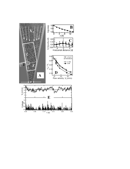
Figure 1: (A) Image of the lower part of the hopper. The flow rate is controlled by varying the outlet $a$. The force transducer is marked ’T’.The large white box indicates the field of view ($\approx 10d$ x $20d$) used to visualize the flow field at $500\thinspace fps$. We measure fast fluctuations in the flow velocity $V_{f}$ at a higher rate of $4000\thinspace fps$ in a field of view whose size is shown by the small square ($2.5d$ x $2.5d$). (B) $V_{f}$ vs. position $z$ going up the wall from the transducer, for $a=4d$. The solid line is the $z$-dependence expected from the continuity equation for an incompressible flow. (C) $V_{f}$ normalized to the velocity at the transducer vs. position going horizontally across from the transducer, for several flow rates. The dashed line is the midpoint of the flow. (D) The normalized standard deviation in flow speed, $\sigma_{V_{f}}/V_{f}$, as a function of $V_{f}$ measured at three locations: at the transducer, $6d$ across from it, and $10d$ up along the wall. (E) Time-dependence of the transducer voltage (proportional to force) and $V_{f}$ for $a=4d$.

Most previous experimental investigations Majumdar05 of force chains in granular flows have been in the quasi-static regime, where grains are essentially in continuous contact. However, some simulations of collisional flows show evidence of large-scale stress-bearing structures. Simulations of pipe flows have observed long-range decay of stress in specific directions Denniston1999 as well as of linear structures made up of frequently colliding particles that transport stress efficiently Ferguson2004 . In studying the initiation of flow by opening the bottom of a container, it was found LudingDuran96 that the flow started with chunks of material falling out of the container; structures labelled ”dynamic arches” held up the rest of the material temporarily, until they broke under the remaining load. A broader understanding of such intermediate-scale stress-bearing structures would help identify the microscopic origins of the non-local rheology reported in a variety of flows GDRMidi2004 ; Pouliquen2004 ; Ertas2002 .

We study the flow of smooth, spherical steel balls of diameter $d=3.125\thinspace mm$ contained in a 2-dimensional hopper. The flow velocity is controlled by varying the width, $a$, of the outlet from $3d$ to $8d$, with the sides held at a fixed angle of $10^{\circ}$ to the vertical. The flow field inside the hopper is measured by imaging at a rate of 500 frames/second ($fps$) the region shown inside the white box in Fig 1A. In Fig 1B, we show the variation of the time-averaged flow velocity, $V_{f}$, as a function of position in the hopper. In the vertical direction, $V_{f}$ varies inversely as the width of the hopper; in the horizontal direction (Fig 1C) the velocity profile shows only a weak spatial dependence with a large slip at the wall, and a maximum at the centre of the channel. The strain rate at the transducer, $\partial V_{f}(x)/\partial z\approx 1.5sec^{-1}$, is nearly independent of the flow rate. Fluctuations about this average velocity profile are anisotropic, with bigger fluctuations along the flow; this is agreement with measurements Choi2004 ; MokaNott2005 at the walls of 3-dimensional dense flows. As the flow velocity is reduced, these fluctuations increase as shown in Fig 1D, where we plot the normalized standard deviation of the flow velocity, $\sigma_{V_{f}}/V_{f}$, against the local flow velocity, $V_{f}$, for three different locations in the cell. At all three locations, fluctuations grow strongly relative to the mean as jamming is approached.

As argued previously, the dynamical origin of these velocity fluctuations must lie in fluctuations in the forces exerted by the walls. We measure this force by means of a normal force transducer embedded in the side wall; the active surface of the transducer is large enough to accommodate exactly one ball. The voltage output of the transducer (Fig. 1E), sampled at $100\thinspace kHz$ is converted into a force by calibration with impacts and static loads of known magnitude. Over the entire range of the flow velocities explored in this article, the forces exerted against the wall are primarily collisional rather than frictional, with balls making repeated but isolated impacts against the transducer. It is not possible to discern the collisional nature of the forces from inspection of video images since the inter-particle separations can be extremely small at these high packing fractions. Simulations Campbell2002 show that small changes in packing fraction can drive a change in the microscopic mechanism of momentum transfer from collisions to friction. We have previously studied Longhi02 the statistics of the impulsive forces as a function of the flow rate, finding that the distribution of forces remained broad at all flow rates, with an exponential tail, just as in static granular media. In order to study the correlation of the flow and the forces, we make measurements of the velocity at $4000fps$, synchronized carefully with the force measurement(Fig. 1E). To achieve these higher imaging speeds without sacrificing spatial resolution, we are obliged to make the velocity measurement in a smaller window as indicated in 1A; measurements are made for several positions of this window: along the wall upstream ($+z$ direction) and downstream ($-z$) of the transducer, as well as normal to the wall ($+x$).

The temporal characteristics of the fluctuations in flow velocity $V_{f}$, are quantified in Fig. 2A, where we show the autocorrelation function $C_{V_{f}}(0,t)$ notation of the velocity at the transducer for several flow speeds. Unlike the magnitude of the fluctuations in $V_{f}$, the decay time is not sensitive to the distance from the jamming threshold: within statistics it is unchanged over a velocity range of $8$ to $34\thinspace cm/s$. (This differs from Ref. Choi2004 where mean-squared particle displacements collapse when plotted against $V_{f}t$, the distance the particle is advected; presumably the difference is that we are in an inertial regime whereas they are in a quasistatic regime where geometry is the dominant consideration). The fluctuations in forces decay faster than the fluctuations in flow velocity, as can be seen in Fig. 2B, where we compare the autocorrelation of $V_{f}$, of force, $F$, and of the collision frequency, $f$.

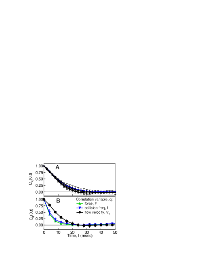
Figure 2: (A) Autocorrelation function, $C_{V_{f}}(0,t)$ of the flow velocity, $V_{f}$ at the transducer $(z=0,x=0)$ as a function of time, $t(msec)$ for openings $a/d=3.04,3.28,4,6,8$. We also include data for $a/d=3.04$ at $z=10d$. The decay time of the autocorrelation does not change as $V_{f}$ changes by a factor $4.25$.(B) The autocorrelation functions of collision frequency, $f$, and average force, $F$, decay faster than that of $V_{f}$. The error bars are standard deviations between 5 data sets, each consisting of 40,000 video frames acquired at $4000fps$.

Even though the collision frequency $f$ and velocity, $V_{f}$ fluctuate on different time scales, their equal-time cross-correlation, $C_{f{V_{f}}}(0,0)$, shown in Fig.3, establishes that these quantities are anti-correlated: higher-than-average collision frequencies are accompanied by negative fluctuations in velocity. The same is true of the correlation between velocity and average force: large forces accompany negative velocity fluctuations. This is implied by the strong positive correlation shown in Fig. 3 of $f$ and $F$ at all flow velocities. This is not a surprising correlation, after all, frequent collisions against the wall generally would indicate greater momentum transfer to the wall, however, the degree of the correlation is very strong. Thus most of the information in force fluctuations is carried by the frequency of collisions, and very little by fluctuations in the magnitude of the impulses.

Figure 3: Equal-time cross correlations $C_{fF}(0,0)$ and $C_{f{V_{f}}}(0,0)$ at the transducer (x=0, z=0) as a function of average flow velocity $V_{f}$, showing the high positive correlation of $F$ and $f$, and the negative correlation between $f$ and $V_{f}$ at all flow velocities.

Is the force at the wall anticorrelated only with the velocity exactly at that point? We investigate this question by plotting in Fig. 4, the equal-time cross-correlation between the collision frequency $f$ at the transducer, and velocity fluctuations at several locations along the wall $C_{f{V_{f}}}(z,0)$, and at other locations normal to the wall $C_{f{V_{f}}}(x,0)$. The greatest anticorrelation is at $x=z=0$, that is, between forces measured at the transducer and $V_{f}$ at that location. These correlations decay anisotropically from this point. Along the wall, the correlation dies off rapidly as a function of $z$, with a decay length of $2$ to $3\thinspace d$. Into the flow, though, the correlation decays approximately linearly in $x$, going to zero only at the far wall. Thus the equal-time correlation is consistent with a high-collision-rate structure that is only a few beads wide in the flow direction, but can span the entire channel transverse to the flow. This can be identified with the collision chains seen in the simulations of Ferguson2004 . Similar structures have also been visualized in the slow flow of soft photoelastic discs in a 2D hopper similar to ours Vivanco .

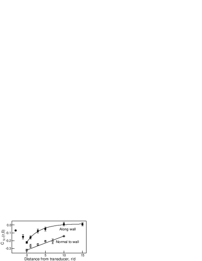
Figure 4: Equal-time cross-correlation between the collision frequency $f$ at the transducer, and velocity fluctuations at different locations along the wall $C_{f{V_{f}}}(z,0)$, and normal to the wall $C_{f{V_{f}}}(x,0)$ (this trace is vertically offset for clarity).

Even though the equal-time correlations shown in Fig. 4 die off quickly in the upstream direction, the high-collision rate events can have an effect far upstream. This is most clearly revealed in the time-dependent cross correlation $C_{f{V_{f}}}(z,t)$ shown in Fig. 5. We first focus on the data ($\bullet$) for $z=0$ . It is apparent that the greatest anticorrelation is at negative times and not at t=0. Thus, the collision rate builds up and is maximum at a time $t_{lag}$ before the flow slows down. There is also a broad peak for positive times, indicating that a period of acceleration is likely to follow, and that there is a suppressed probability for the formation of another collisional ”arch” immediately after. The other curves shown in Fig. 4 represent $C_{f{V_{f}}}(z,t)$ for increasing values of $z$, i.e. for positions along the wall, upstream from the transducer. The anticorrelation at the minimum of the curve $(t=t_{lag})$ is larger, and diminishes much slower with distance, than does the anticorrelation at $t=0$. Thus even though the equal-time correlation indicates a thin, local structure, the effect on the flow is extremely long-range. $t_{lag}(z)$, the time required for the information propagate a distance $z$ upstream, is shown in the inset. The slope represents the velocity at which the force information propagates upstream; this velocity is more than an order of magnitude greater than the flow speed, and is comparable to $d\langle f\rangle$, the particle diameter multiplied by the mean collision frequency. Thus, the communication is very coherent, akin to a longitudinal sound mode.

Figure 5: The time-dependent cross correlation $C_{f{V_{f}}}(z,t)$ against delay time, $t$ for different $z$ along the wall. The maximum of the negative correlation occurs at a negative delay time $t_{lag}$. Inset: $t_{lag}$ versus distance, $z/d$ ($\bullet$) and $x/d$ ($\circ$).

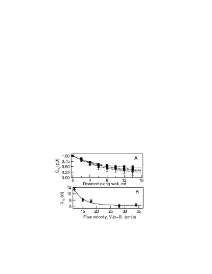
Figure 6: (A) Equal-time spatial cross correlations $C_{V_{f}}(z,0)$ between velocities $V_{f}$ at different $z$ along the wall. (B) The distance, $\lambda_{1/2}$, at which the spatial correlation decays to 1/2, as a function of flow velocity, $V_{f}$.

This long-range effect of clogging by transient arches leads to a flow with pronounced spatial correlations: the extreme version of this occurs when a stable arch forms across the channel - the flow comes to a halt everywhere in the hopper. However, there is a continuous approach to this limit as the flow velocity is slowed down towards jamming. This is shown in Fig. 6A where we plot for several flow speeds, the spatial correlation of the velocity field, $C_{V_{f}}(z,0)$, as a function of position along the wall. The correlation decays slower in space as the flow slows down. This is demonstrated in Fig. 6B where we show the distance, $\lambda_{1/2}$, at which the correlation falls to $1/2$.

Thus the approach to jamming is characterized by both an increasing correlation length scale in the velocity fluctuations (Fig. 6) as well as an increasing amplitude (Fig. 1D) for the fluctuations. We have also previously observed in this geometry Longhi02 that a time-scale diverges: the collision time distribution goes to a power-law with an exponent of $-3/2$. The driving force for the slow-down and arrest of the flow appears to be collisionally stabilized structures reminiscent of the force chains observed in static granular packings. In our experiments, these collision chains are not directly observed but are identified via their anticorrelation with the velocity field: a high collision rate immediately precedes the slowing down of the flow. At any instant, the correlations indicate that these transient structures are thin in the flow direction and long-ranged transverse to the flow. The effect of these localized structures is propagated rapidly to upstream parts of the flow, signalling a temporary clogging of the flow downstream. We are currently exploring similar phenomena in 3D flows 3Dflow , where force measurements reveal both collisional and frictional regimes.

We thank F. Rouyer for her help with the experiment, and B. Chakraborty, A. Ferguson, S. Tewari, J.W. Landry, A.D. Dinsmore for useful discussions. We acknowledge support from NSF-DMR 0305396, and NSF-MRSEC 0213695.

References

- (1) P. Dantu, Ann. Pont Chaussees IV, 144 (1967); T. Travers et al., Europhys. Lett. 4, 329 (1987).
- (2) C. H. Liu et al., Science 269, 513 (1995).
- (3) D. Howell, R. P. Behringer, C. Veje, Phys. Rev. Lett. 82, 5241 (1999).
- (4) T. Majumdar, R.P. Behringer, Nature, (2005).
- (5) C. Denniston, H. Li, Phys. Rev. E 59, R3289 (1999).
- (6) A. Ferguson, B. Fisher and B. Chakraborty, Europhys. Lett. 66, 277 (2004).
- (7) S. Luding, J. Duran, E. Clement, J. Rajchenbach, J. Phys. I 6, 823 (1996); J. Duran et al., Phys. Rev. E 53 1923 (1996).
- (8) GDRMidi, Eur. Phys. J. E 14, 34 (2004)
- (9) D. Ertas, T.C. Halsey, Europhys. Lett. 60, 931 (2002).
- (10) O. Pouliquen, Phys. Rev. Lett. 93, 248001 (2004).
- (11) J. Choi, A. Kudrolli, R.R. Rosales, M. Bazant, Phys. Rev. Lett. 92, 174301 (2004).
- (12) S. Moka, P. Nott, Phys. Rev. Lett. 95, 068003 (2005).
- (13) C.S. Campbell, J. Fluid Mech., 465, 261 (2002).
- (14) E. Longhi, N. Easwar, N. Menon, Phys. Rev. Lett. 89, 045501 (2002).
- (15) We denote the time- and space-correlation of variables and by where . The angle brackets, , denote an average over the initial time, ; since the system is not homogeneous in space, no average is taken over the initial position, typically chosen to be the location of the transducer. The subscript is not repeated for autocorrelation functions.
- (16) F. Vivanco, F. Melo, S. Rica, private communication.
- (17) E. Seitaridou, E. Gardel, N. Easwar, N. Menon, in preparation.