Capacitance Calculations Using the Lattice Green Function in Two Dimensions

Abstract

We show how to use the lattice Green function to calculate capacitances in two dimensions with boundary conditions at infinity. It is shown how to calculate coefficients of capacitance and induction from the lattice Green function. A general analysis of two arbitrary conductors is carried out. It is shown how the calculations can be simplified in the case of identical conductors when certain symmetry conditions are met. Example calculations for a parallel and coplanar stripline are shown. The use of the two conductor formulas for the case of three or more conductors is discussed.

I introduction

In a two dimensional homogeneous and unbounded space, the Poisson equation and its solution are given by

$$\nabla^{2}\phi(\vec{r})=-\frac{\rho(\vec{r})}{\epsilon}$$ (1)

$$\phi(\vec{r})=\frac{1}{2\pi\epsilon}\int\ln\left(\frac{r_{0}}{|\vec{r}-\vec{r}^{\prime}|}\right)\rho(\vec{r}^{\prime})\;d\vec{r}^{\prime}$$ (2)

When the charge density is known then eq. 2 reduces the problem of finding the potential at any point in space to a simple integration. A more interesting and difficult problem occurs when the charge density is not known. An example of such a probelm is the case of two conductors each of which is held at some constant potential. Eq. 2 is then an integral equation for the charge density on the conductors and it is difficult to solve analytically in all but a few simple cases. Many approximation schemes have been devised to deal with this problem and in most cases the solution must be found numerically. One commonly used approach is to discretize eq. 2, thereby turning it into a matrix equation, which can then be solved using standard techniques. The disadvantage of this approach is that it is an approximation of the continuous as well as the discrete version of the problem, i.e. it is an approximation in both continuous and discrete space.

An alternative approach is to formulate the entire problem in a discrete space. Physically the model is an infinite square lattice with capacitors connecting the nodes. Sets of adjacent nodes, that correspond to discretized versions of conductors, are held at constant potential and the problem is to find the charges at those nodes. Mathematically this approach is equivalent to replacing the Laplacian in eq. 1 with its finite difference approximation. The discrete space version of eq. 1 is then

$$\sum_{m}L_{nm}\phi(\vec{r}_{m})=-\frac{\lambda(\vec{r}_{n})}{\epsilon}$$ (3)

where $\vec{r}_{n}$ is a lattice vector of the form: $\vec{r}_{n}=n_{1}\vec{a}_{1}+n_{2}\vec{a}_{2}$, $n_{i}=$integer, $\vec{a_{i}}=a\hat{x}_{i}$ and $a=$lattice spacing. $\lambda(\vec{r}_{n})$ is the linear charge density at node $\vec{r}_{n}$. $L_{nm}$ is a matrix element of the lattice Laplacian and is defined as

$$L_{nm}=-4\delta(\vec{r}_{n},\vec{r}_{m})+\sum_{i=1}^{2}\left[\delta(\vec{r}_{n}+\vec{a}_{i},\vec{r}_{m})+\delta(\vec{r}_{n}-\vec{a}_{i},\vec{r}_{m})\right]$$ (4)

To simplify the notation we will write eq. 3 in the following form

$$\sum_{m}L_{nm}\phi(\vec{r}_{m})=-q(\vec{r}_{n})$$ (5)

where $L_{nm}$ now has units of capacitance and $q(\vec{r}_{n})$ is a charge at node $\vec{r}_{n}$. The solution of this equation for $\phi(\vec{r}_{n})$ is

$$\phi(\vec{r}_{n})=\sum_{m}G_{nm}\,q(\vec{r}_{m})$$ (6)

where $G_{nm}$ is a matrix element of the Green function with units of elastance. The Green function in this problem is defined as, $G=-L^{-1}$, where $L$ is the lattice Laplacian operator. Eq. 6 is the discrete space version of eq. 2.

$G_{nm}$ is a function of $|\vec{r}_{n}-\vec{r}_{m}|$ only, so a more convenient notation for eq. 6 is

$$\phi(n_{1},n_{2})=\sum_{m_{1},m_{2}}G(p_{1},p_{2})\,q(m_{1},m_{2})$$ (7)

where $p_{1}=|n_{1}-m_{1}|$ and $p_{2}=|n_{2}-m_{2}|$. The problem with this equation however, is that $G(p_{1},p_{2})$ is infinite for all values of $p_{1}$ and $p_{2}$. This same problem occurs in the continuous case, eq. 2, when the reference point for the potential, $r_{0}$, is taken to infinity. The way around this problem is to use $g(p_{1},p_{2})=G(0,0)-G(p_{1},p_{2})$ which is finite for all values of $p_{1}$ and $p_{2}$ Hollos and Hollos (2005a, b). Eq. 7 then becomes

$$\phi(n_{1},n_{2})=-\sum_{m_{1},m_{2}}g(p_{1},p_{2})\,q(m_{1},m_{2})$$ (8)

This equation will solve the original problem as long as all the charges sum to zero. We will now show how to use this formalism to calculate the capacitance between conductors in two dimensions.

II general analysis of two conductors

Consider the case of two conductors discretized so that there are $n_{1}$ charges on conductor 1 and $n_{2}$ charges on conductor 2. The conductors are held at constant potentials $\phi_{1}$ and $\phi_{2}$. The equation for this system is written as follows

$$-\left(\begin{array}[]{cc}\mathbf{G}_{11}&\mathbf{G}_{12}\\ \mathbf{G}_{21}&\mathbf{G}_{22}\end{array}\right)\left(\begin{array}[]{c}\vec{\mathbf{q}}_{1}\\ \vec{\mathbf{q}}_{2}\end{array}\right)=\left(\begin{array}[]{c}\phi_{1}\vec{\mathbf{e}}_{1}\\ \phi_{2}\vec{\mathbf{e}}_{2}\end{array}\right)$$ (9)

$\vec{\mathbf{q}}_{i}$ is an $n_{i}$ dimensional vector of the charges on conductor $i$. $\vec{\mathbf{e}}_{i}$ is an $n_{i}$ dimensional vector with all elements equal to 1. $\mathbf{G}_{ii}$ is an $n_{i}\,x\,n_{i}$ matrix that gives the contribution of the charges on conductor $i$ to the potential of the conductor. $\mathbf{G}_{ij}$ is an $n_{i}\,x\,n_{j}$ matrix that gives the contribution of the charges on conductor $j$ to the potential of conductor $i$. The elements of $\mathbf{G}_{ij}$ depend only on the absolute separation of two charges therefore it will always be true that $\mathbf{G}_{ij}=\mathbf{G}_{ji}^{T}$.

As a simple example, take two conductors discretized such that there are two charges on both conductors. Let the charges on conductor 1 be at $(0,0)$ and $(0,1)$ and the charges on conductor 2 be at $(2,0)$ and $(3,0)$. The $\mathbf{G}_{ij}$ submatrices in eq. 9 will then be

$$\mathbf{G}_{11}=\mathbf{G}_{22}=\left(\begin{array}[]{cc}0&g(1,0)\\ g(1,0)&0\end{array}\right)$$ (10)

$$\mathbf{G}_{12}=\mathbf{G}_{21}^{T}=\left(\begin{array}[]{cc}g(2,0)&g(3,0)\\ g(2,1)&g(3,1)\end{array}\right)$$ (11)

In general, to calculate the capacitance between two conductors the matrix in eq. 9 needs to be inverted in order to find the charges $\vec{\mathbf{q}}_{1}$, and $\vec{\mathbf{q}}_{2}$. The matrix is easily inverted if it is first factored into a product of an upper and lower triangular matrix. This can be done in two ways

$$\left(\begin{array}[]{cc}\mathbf{G}_{11}&\mathbf{G}_{12}\\ \mathbf{G}_{21}&\mathbf{G}_{22}\end{array}\right)=\left(\begin{array}[]{cc}\mathbf{I}&\mathbf{0}\\ \mathbf{G}_{21}\mathbf{G}_{11}^{-1}&\mathbf{I}\end{array}\right)\left(\begin{array}[]{cc}\mathbf{G}_{11}&\mathbf{G}_{12}\\ \mathbf{0}&\mathbf{G}_{22}-\mathbf{G}_{21}\mathbf{G}_{11}^{-1}\mathbf{G}_{12}\end{array}\right)$$ (12)

or

$$\left(\begin{array}[]{cc}\mathbf{G}_{11}&\mathbf{G}_{12}\\ \mathbf{G}_{21}&\mathbf{G}_{22}\end{array}\right)=\left(\begin{array}[]{cc}\mathbf{I}&\mathbf{G}_{12}\mathbf{G}_{22}^{-1}\\ \mathbf{0}&\mathbf{I}\end{array}\right)\left(\begin{array}[]{cc}\mathbf{G}_{11}-\mathbf{G}_{12}\mathbf{G}_{22}^{-1}\mathbf{G}_{21}&\mathbf{0}\\ \mathbf{G}_{21}&\mathbf{G}_{22}\end{array}\right)$$ (13)

Inverting these upper and lower triangular matrices then leads to two sets of equations for the submatrices of the inverse. From eq. 12 we get

$$(\mathbf{G}^{-1})_{11} = \mathbf{G}_{11}^{-1}+\mathbf{G}_{11}^{-1}\mathbf{G}_{12}(\mathbf{G}_{22}-\mathbf{G}_{21}\mathbf{G}_{11}^{-1}\mathbf{G}_{12})^{-1}\mathbf{G}_{21}\mathbf{G}_{11}^{-1}$$ (14)

$$(\mathbf{G}^{-1})_{12} = -\mathbf{G}_{11}^{-1}\mathbf{G}_{12}(\mathbf{G}_{22}-\mathbf{G}_{21}\mathbf{G}_{11}^{-1}\mathbf{G}_{12})^{-1}$$

$$(\mathbf{G}^{-1})_{21} = -(\mathbf{G}_{22}-\mathbf{G}_{21}\mathbf{G}_{11}^{-1}\mathbf{G}_{12})^{-1}\mathbf{G}_{21}\mathbf{G}_{11}^{-1}$$

$$(\mathbf{G}^{-1})_{22} = (\mathbf{G}_{22}-\mathbf{G}_{21}\mathbf{G}_{11}^{-1}\mathbf{G}_{12})^{-1}$$

and from eq. 13 we get

$$(\mathbf{G}^{-1})_{11} = (\mathbf{G}_{11}-\mathbf{G}_{12}\mathbf{G}_{22}^{-1}\mathbf{G}_{21})^{-1}$$ (15)

$$(\mathbf{G}^{-1})_{12} = -(\mathbf{G}_{11}-\mathbf{G}_{12}\mathbf{G}_{22}^{-1}\mathbf{G}_{21})^{-1}\mathbf{G}_{12}\mathbf{G}_{22}^{-1}$$

$$(\mathbf{G}^{-1})_{21} = -\mathbf{G}_{22}^{-1}\mathbf{G}_{21}(\mathbf{G}_{11}-\mathbf{G}_{12}\mathbf{G}_{22}^{-1}\mathbf{G}_{21})^{-1}$$

$$(\mathbf{G}^{-1})_{22} = \mathbf{G}_{22}^{-1}+\mathbf{G}_{22}^{-1}\mathbf{G}_{21}(\mathbf{G}_{11}-\mathbf{G}_{12}\mathbf{G}_{22}^{-1}\mathbf{G}_{21})^{-1}\mathbf{G}_{12}\mathbf{G}_{22}^{-1}$$

In terms of these submatrices the charges on the two conductors are given by

$$\vec{\mathbf{q}}_{1} = -\phi_{1}(\mathbf{G}^{-1})_{11}\vec{\mathbf{e}}_{1}-\phi_{2}(\mathbf{G}^{-1})_{12}\vec{\mathbf{e}}_{2}$$ (16)

$$\vec{\mathbf{q}}_{2} = -\phi_{1}(\mathbf{G}^{-1})_{21}\vec{\mathbf{e}}_{1}-\phi_{2}(\mathbf{G}^{-1})_{22}\vec{\mathbf{e}}_{2}$$

The total charge on conductor $i$ is $Q_{i}=\vec{\mathbf{e}}_{i}^{T}\vec{\mathbf{q}}_{i}$, so if the first equation is multiplied by $\vec{\mathbf{e}}_{1}^{T}$ and the second equation by $\vec{\mathbf{e}}_{2}^{T}$ then we get a set of equations relating the total charges on each conductor to their potentials.

$$Q_{1} = c_{11}\phi_{1}+c_{12}\phi_{2}$$ (17)

$$Q_{2} = c_{12}\phi_{1}+c_{22}\phi_{2}$$

The coefficients $c_{ii}$ are known as coefficients of capacitance and $c_{12}$ is known as a coefficient of induction. The coefficient $c_{ij}$ is equal to the negative of the sum of all the elements in the matrix $(\mathbf{G}^{-1})_{ij}$.

$$c_{ij}=-\vec{e}_{i}^{T}(G^{-1})_{ij}\vec{e}_{j}$$ (18)

From eq. 14 and 15 it is clear that $(\mathbf{G}^{-1})_{ij}=(\mathbf{G}^{-1})_{ji}^{T}$ and therefore $c_{ij}=c_{ji}$. Since the potential and the charge of a conductor will have the same sign, we have the condition $c_{ii}>0$. Also since the charge induced by a conductor will have a sign opposite to the potential of the conductor, we have $c_{12}<0$.

In addition to eq. 17 we have the requirement that the sum of all the charges must equal zero, $Q_{1}+Q_{2}=0$. This means that we can set $Q_{1}=Q$ and $Q_{2}=-Q$ in eq. 17 and solve for the potentials.

$$\phi_{1} = \left(\frac{c_{22}+c_{12}}{c_{11}c_{22}-c_{12}^{2}}\right)\,Q$$ (19)

$$\phi_{2} = -\left(\frac{c_{11}+c_{12}}{c_{11}c_{22}-c_{12}^{2}}\right)\,Q$$

The ratio of the two potentials is then given by

$$\frac{\phi_{1}}{\phi_{2}}=-\left(\frac{c_{22}+c_{12}}{c_{11}+c_{12}}\right)$$ (20)

The capacitance between the two conductors can then be expressed in terms of the $c_{ij}$ coefficients as follows.

$$C=\frac{Q}{\phi_{1}-\phi_{2}}=\frac{c_{11}c_{22}-c_{12}^{2}}{c_{11}+c_{22}+2c_{12}}$$ (21)

Note that the denominator, $c_{11}+c_{22}+2c_{12}$ is equal to the negative of the sum of all the elements of the inverse of the Green function matrix in eq. 9 and that the $c_{ij}$’s are functions only of the geometry of the two conductors. Eq. 21 can be used to calculate the capacitance between two conductors of arbitrary size, shape and orientation once the $c_{ij}$ coefficients have been calculated. Each conductor may consist of more than one disconnected piece as long as each piece is held at the same potential. We now look at the special case of two identical conductors, i.e. both conductors have the same size and shape.

III two identical conductors

For two conductors of the same size and shape the calculation of capacitance and charge distribution can be simplified in those cases where the coefficients of capacitance are equal. We begin then by examining what conditions are required to get $c_{11}=c_{22}$.

Since $c_{ii}$ is equal to the sum of the elements of the $(\mathbf{G}^{-1})_{ii}$ matrix, the two $c_{ii}$ will automatically be equal if the two $(\mathbf{G}^{-1})_{ii}$ matrices are equal. For identical conductors it will always be true that $\mathbf{G}_{11}=\mathbf{G}_{22}$ so that the expressions for $(\mathbf{G}^{-1})_{ii}$ in equations 14 and 15 become

$$(\mathbf{G}^{-1})_{11} = (\mathbf{G}_{11}-\mathbf{G}_{12}\mathbf{G}_{11}^{-1}\mathbf{G}_{21})^{-1}$$ (22)

$$(\mathbf{G}^{-1})_{22} = (\mathbf{G}_{11}-\mathbf{G}_{21}\mathbf{G}_{11}^{-1}\mathbf{G}_{12})^{-1}$$

These expressions are only equal if $\mathbf{G}_{12}=\mathbf{G}_{21}=\mathbf{G}_{12}^{T}$ i.e. $\mathbf{G}_{12}$ must be symmetric.

$\mathbf{G}_{12}$ is a function only of the distance between charges on the two conductors therefore it can be made symmetric if it is possible to take one conductor to the other by a reflection about a horizontal plane, a vertical plane, both a horizontal and vertical plance, or a diagonal plane. Figure 1 shows the case of two conductors that can be made congruent through reflection about the vertical plane $ab$ followed by reflection about the horizontal plane $cd$. The point $1$ is taken to the point $1^{\prime}$ so that these charges will be equal and all charges to the right of point $1$ will equal the corresponding charges to the left of point $1^{\prime}$.

With $\mathbf{G}_{12}$ symmetric we have $c_{11}=c_{22}$ and the equations for the general case simplify. From eq. 20 we get $\phi_{1}=-\phi_{2}=\phi$ and the potential is related to the charge as follows

$$\phi=\frac{Q}{c_{11}-c_{12}}$$ (23)

The capacitance is then given by

$$C=\frac{c_{11}-c_{12}}{2}$$ (24)

For this symmetric case, each charge on one conductor will have a corresponding equal and opposite charge on the other conductor so that in eq. 9 we get $\vec{\mathbf{q}}_{1}=-\vec{\mathbf{q}}_{2}=\vec{\mathbf{q}}$ and the equation reduces to

$$(\mathbf{G}_{12}-\mathbf{G}_{11})\vec{\mathbf{q}}=\phi\vec{\mathbf{e}}$$ (25)

The total charge on one conductor is then related to the potential as follows

$$Q=\phi\vec{\mathbf{e}}^{T}(\mathbf{G}_{12}-\mathbf{G}_{11})^{-1}\vec{\mathbf{e}}$$ (26)

Comparing this equation with eq. 23 gives

$$c_{11}-c_{12}=\vec{\mathbf{e}}^{T}(\mathbf{G}_{12}-\mathbf{G}_{11})^{-1}\vec{\mathbf{e}}$$ (27)

The capacitance can therefore be calculated from the sum of all the elements of the inverse of the matrix $\mathbf{G}_{12}-\mathbf{G}_{11}$.

As examples, we will now consider the case of the parallel stripline and the coplanar stripline. A parallel stripline and the potential surrounding it is shown in Fig. 2. The upper and lower plates are at potentials +1 and -1 respectively. A plot of the capacitance as a function of the ratio of the width of the plates to their separation is shown in fig. 3. For each ratio the resolution was increased (lattice constant decreased) until the capacitance value appeared to converge. Fig. 4 shows the convergence for the ratios 1, 5 and 10 as a function of the number of charges in the plates. With $r$ equal to the ratio of the width to the separation, the following equation fits the plot of the capacitance in fig. 3 with a correlation coefficient of 0.999998.

$$C=r+1.12863+0.202069\;\ln(r-0.0964012)$$ (28)

This equation agrees well with previous work by Wheeler Wheeler (1965). The coplanar stripline and the potential surrounding it is shown in fig. 5. The left and right plates are at potentials -1 and +1 respectively, with a plate separation of 1/5 the width of a plate. A plot of the capacitance as a function of the ratio of width to separation of the plates is shown in fig. 6.

IV conclusion

The formalism discussed above can easily be extended to the case of three or more conductors. The Green function matrix inverse formulas in eq. 14 and 15 can be applied iteratively in this case. Start with any two conductors, generate $G_{11}$, $G_{22}$, $G_{12}$, and then use one of the sets of equations to find the inverse. This inverse then becomes $G_{11}^{-1}$ in eq. 14 when the next conductor is included, for which we have a new $G_{22}$ and $G_{12}$, with $G_{12}$ connecting the new conductor with the previous two. This makes it possible to look at the effect of changes in the placement of a new conductor (or a single charge) with respect to a set of conductors without major recalculation efforts.

Another theorem that may be useful in the case of three or more conductors is Green’s Reciprocation Theorem. In its simplest form the theorem says that if we have a set of $N$ conductors at potentials $\phi_{i}$ and charges $Q_{i}$ ($i=1,\,\ldots\,N$) and then take those same conductors at new potentials $\phi_{i}^{\prime}$ and charges $Q_{i}^{\prime}$ then the following equation holds

$$\sum_{i=1}^{N}Q_{i}\,\phi_{i}^{\prime}=\sum_{i=1}^{N}Q_{i}^{\prime}\,\phi_{i}$$ (29)

This theorem is easily proven by writing out equations similar to eq. 17 for the $Q_{i}$ and $Q_{i}^{\prime}$. The equations for $Q_{i}$ are multiplied by $\phi_{i}^{\prime}$ and the equations for $Q_{i}^{\prime}$ are multiplied by $\phi_{i}$. Summing the two sets of equations then gives eq. 29.

The capacitance calculations we have discussed can also be applied to finding the energy and forces on conductors and to calculating transmission line impedances. The energy of a set of $N$ conductors with charges $Q_{i}$ and potentials $\phi_{i}$ is Jackson (1975)

$$W=\frac{1}{2}\sum_{i=1}^{N}Q_{i}\,\phi_{i}=\frac{1}{2}\sum_{i=1}^{N}\sum_{j=1}^{N}c_{ij}\,\phi_{i}\,\phi_{j}$$ (30)

To calculate the force on a conductor in a given direction, with all conductors held at constant potential, we displace the conductor in that direction and then calculate the new $c_{ij}^{\prime}s$ and the new energy. The force is then the change in energy divided by the lattice constant.

The impedance of the transmission line formed by two conductors is given by the equation

$$Z=\frac{\eta}{C}$$ (31)

where $\eta$ is the characteristic impedance of the medium, given by $\eta=\sqrt{\mu/\epsilon}$, and $C$ is the capacitance given by eq. 21. Note that $C$ is treated here as a pure number i.e. it is not scaled by $\epsilon$.

Formulating electrostatics problems and their solution entirely in discrete space has many advantages. This was first recognized in a well known paper by Courant et al Courant et al. (1967) in which they examined the solution of elliptic partial differential equations and their corresponding difference equations. They were able to show that the difference equation solution does converge to the solution of the differential equation and that some questions, such as the existence of solutions, are more easily answered by looking at the difference equation. It appears that in many cases the theorems and methods developed for continuous space problems can be translated over into discrete space. It also seems to us that the possibility exists for discovering new theorems or generalizations of existing theorems, such as Thompson-Lampard Thompson and Lampard (1956), by approaching problems from a discrete space point of view. Opportunities for more research in this area certainly exist.

Figure 1: Symmetry example.

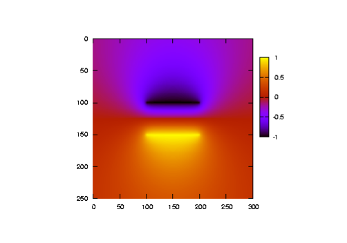
Figure 2: Parallel stripline potential: 100 charges/plate, separation is 1/2 plate width.

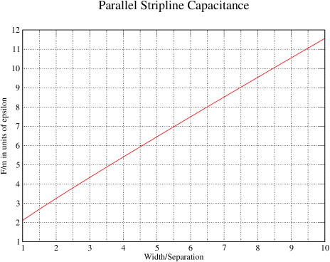
Figure 3: Parallel stripline capacitance: F/m in units of epsilon vs. width/separation. 1000 charges per plate.

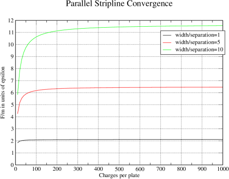
Figure 4: Parallel plate convergence: F/m in units of epsilon vs. charges per plate

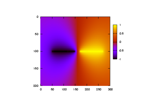
Figure 5: Coplanar stripline potential: 100 charges/plate, separation is 1/5 plate width.

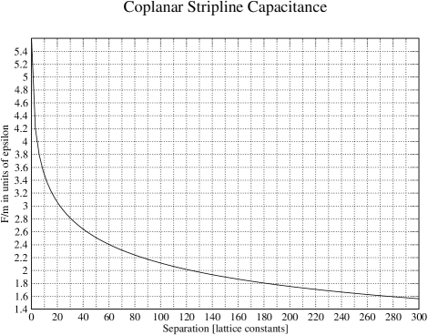
Figure 6: Coplanar stripline capacitance: F/m in units of epsilon vs. separation in units of lattice constants. 300 charges per plate.

References

• Hollos and Hollos (2005a) S. Hollos and R. Hollos, Some square lattice green function formulas (2005a), eprint cond-mat/0508779.
• Hollos and Hollos (2005b) S. Hollos and R. Hollos, The lattice green function for the poisson equation on an infinite square lattice (2005b), eprint cond-mat/0509002.
• Wheeler (1965) H. A. Wheeler, IEEE Trans. Microwave Theory Tech. MTT-13, 172 (1965).
• Jackson (1975) J. D. Jackson, Classical Electrodynamics (Wiley, 1975), 2nd ed.
• Courant et al. (1967) R. Courant, K. Friedrichs, and H. Lewy, IBM Journal of Research and Development 11, 215 (1967), english translation. Originally appeared in Mathematische Annalen, Vol 100, p32-74, 1928.
• Thompson and Lampard (1956) A. M. Thompson and D. G. Lampard, Nature 177, 888 (1956).
Refer to caption