Energy dependence on fractional charge for
strongly interacting subsystems

Abstract

The energies of a pair of strongly-interacting subsystems with arbitrary noninteger charges are examined from closed and open system perspectives. An ensemble representation of the charge dependence is derived, valid at all interaction strengths. Transforming from resonance-state ionicity to ensemble charge dependence imposes physical constraints on the occupation numbers in the strong-interaction limit. For open systems, the chemical potential is evaluated using microscopic and thermodynamic models, leading to a novel correlation between ground-state charge and an electronic temperature.

Associating fractional charges with individual atoms is a habitual part of our every-day thinking about condensed and molecular matter. Indeed, characterizing the energetics of such systems in terms of dynamically-evolving charges is now recognized as key to understanding the atomic-scale behavior of complex processes ranging from alloying to motor protein function to molecular logic gate operation CTRef . Compounding the difficulty of the problem is that the instantaneous redistribution of charge occurs under the influence of strong interactions among subsystems of atoms and molecules.

Historically, it was assumed that quadratic electrostatic interactions constitute a reasonable representation of the energy dependence on fractional charge Rappé and Goddard (1991), independent of the strength of interaction. However, the inadequacy of the historical assumption had been highlighted by the work of Perdew et al. (hereafter referred to as PPLB) PPLB , where a linear dependence was found for weakly interacting subsystems. This was found by considering an open subsystem that was allowed to weakly interact and exchange electrons with a reservoir of electrons PerdewNATO . For a diatomic molecule, the weak interaction restriction implies that the theory is valid only at large internuclear separations $R$. PPLB considered an atom A as a subsystem in its neutral state with $M$ electrons and energy $E_{M}$ that becomes anionic by fractional charge $q$, where the anionic state with $M+1$ electrons has energy $E_{M+1}$. The energy $E_{\rm A}(q)$ was shown to be the ensemble average

$$E_{\rm A}(q)=E_{M}+\omega\,(E_{M+1}-E_{M})\,,$$ (1)

with $\omega\sim\omega_{\rm PPLB}=-q\geq 0$. This result established a seminal extension of density functional theory (DFT) to fractional numbers of electrons Persp . The energy $E_{\rm A}(q)$ is manifestly linear in $q$, in contrast to the historically-assumed quadratic dependence. A direct consequence of Eq. (1) is that the associated microscopic chemical potential $\mu=-dE_{\rm A}(q)/dq$ exhibits a discontinuity with respect to charge $q$ PPLB . The veracity of both limits has been confirmed numerically by Ciosłowski and Stefanov CioStef . In this Letter, we construct a novel, analytic model explicitly linking the weak (linear) and strong (quadratic) interaction limits, and characterize the corresponding behavior of $\mu$ with respect to $q$. As discussed below, this requires the definition of interacting “atom-in-molecule” (AIM) subsystems and associated fractional charges. While these definitions are not unique PAN05 , and many physically-reasonable alternatives are possible HarrisCharge ; GhosezPerov ; CohenWass ; WuVoorhis , our results are independent of the details of a specific AIM approach.

Previous attempts to extend PPLB’s formal results to moderate and strong interactions have recast the problem in terms of charge resonances CT-EVB ; Nalewajski (1998); ToddM ; ToddMII of a closed system composed of A$+\cal{R}$, where $\cal{R}$ represents the electron reservoir. In the charge resonance view, one supposes that special wavefunctions can be constructed such that the charges on the subsystems are integers Warshel ; MullikenDi ; PhillipsRMP ; CoulsonRedei ; AdelHersch . Interpreting PPLB in the language of resonances, the state designated as $M$ for A corresponds to both A and $\cal{R}$ being neutral (covalent resonance), while $M+1$ corresponds to A being anionic and $\cal{R}$ being cationic (ionic resonance), leaving the total system neutral.

Extending this picture to the intermediate interaction regime CT-EVB ; fn1 , ${\cal R}$ ceases to be a structureless reservoir of electrons, but must instead be viewed as a structured subsystem B at a finite separation $R$ from A. This subsystem may be an atom, molecule, or bulk material. Although several two-state valence bond models have been developed in this limit CT-EVB ; Nalewajski (1998); ToddM ; ToddMII , previous attempts to extend the valence bond approach to the strong interaction limit have proven unsuccessful.

A complete generalization of PPLB to the strong interaction limit can be attained by transforming from the resonance-state basis to an ensemble or spectral representation PerdewNATO . Let $\hat{H}$ denote the hamiltonian for the closed system AB with eigenstates $\{\Psi_{k}\}$ and eigenenergies $\{E_{k}\}$. Let $\Psi$ be any arbitrary trial wavefunction with $\langle\Psi|\Psi\rangle=1$. The variational energy can then be expressed in a spectral representation,

$$\langle\Psi|\hat{H}|\Psi\rangle=\sum_{k}\omega_{k}E_{k}\,,$$ (2)

where the $\omega_{k}=|\langle\Psi|\Psi_{k}\rangle|^{2}$ are occupation numbers. Now we express $\Psi$ as a linear combination of resonance states $\{\psi_{i}\}$ with coefficients $\{c_{i}\}$, such that $\Psi=\sum_{i}c_{i}\psi_{i}$. The eigenvectors $\bm{C}_{k}$ are the specific values of coefficients corresponding to the eigenstates. The basis rotation from the $\{\psi_{i}\}$ to the $\{\Psi_{k}\}$ in terms of the $\bm{C}_{k}$ lead to occupation numbers

$$\omega_{k}=|\sum_{i}c_{i}^{*}{C}_{ik}|^{2}\,.$$ (3)

These occupation numbers give rise to piecewise linearity in the energy when AB dissociates PPLB ; YZA-Frac . Specializing to a two-state model, we define the ionicity $\gamma$ as the ratio $c_{1}/c_{0}$, where $c_{0}$ and $c_{1}$ are the coefficients for the covalent and ionic resonances, respectively. Let $\gamma_{\rm gs}$ and $\gamma_{\rm xs}$ denote the eigenionicities corresponding to the ground- and excited-state values of $c_{1}/c_{0}$, at some chosen separation $R$ CT-EVB . The dependence of the energy $E(\gamma)$ on an externally-imposed ionicity $\gamma$ is then given by

$$E(\gamma;R) = E_{\rm gs}(R)$$ (4)

$$+\,\omega(\gamma;\gamma_{gs}(R),\gamma_{xs}(R))\left(E_{\rm xs}(R)-E_{\rm gs}(R)\right)\,,$$

with

$$\omega(\gamma;\,\gamma_{\rm gs},\gamma_{\rm xs})=\frac{(\gamma-\gamma_{\rm gs})^{2}}{(\gamma-\gamma_{\rm gs})^{2}+\big{(}\frac{1-\gamma_{\rm gs}^{2}}{\gamma_{\rm xs}^{2}-1}\big{)}\left(\gamma-\gamma_{\rm xs}\right)^{2}}\,.$$ (5)

This occupation number governs how the energy of AB changes when its ionicity is forced to deviate from its ground-state value (Fig. 1). Importantly, this result is independent of the strength of the interaction. As is necessary physically, $\omega=0$ when $\gamma=\gamma_{\rm gs}$, and $\omega=1$ when $\gamma=\gamma_{\rm xs}$. Moreover, both extrema are represented, as the derivative of $\omega$ with respect to $\gamma$ is zero when evaluated at either $\gamma_{\rm gs}$ or $\gamma_{\rm xs}$ (Fig. 2a).

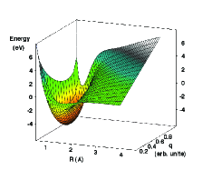
Figure 1: (Color) Energy of a heteronuclear diatomic molecule as a function of bond length and charge as modeled by Eq. (4). The charge dependence is linear as the molecule dissociates PPLB , while being quadratic near the ground-state charge when $R$ is near equilibrium values Rappé and Goddard (1991); CioStef . The constituent atoms interact strongly near equilibrium.

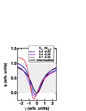
(a) (b)

Figure 2: (a) (Color online) Intermediate limit of Eq. (5). The extrema correspond to $\gamma=\gamma_{\rm gs}$ and $\gamma=\gamma_{\rm xs}=-1/\gamma_{\rm gs}$. (b) Relationship between charge and ionicity in the strong interaction regime for the two-state model and the atom-in-molecule model of Ref. CT-EVB . $S_{\rm ci}$ and $\delta N_{\rm ci}^{*}$ are AIM parameters entering the $\gamma-q$ relation in the strong interaction regime. The gray zone corresponds to the physical range of $q$ between 0 and 1.

Equation (5) is expressed in terms of the ionicity $\gamma$. In order to complete the model it is necessary to eliminate this quantum mechanical parameter in favor of the physical charge $q$ Fano . This can be accomplished through an AIM decomposition CT-EVB ; CioStef . The relation between $\gamma$ and $q$ in the strong interaction regime is illustrated in Fig. 2b. It reduces to $\gamma=\pm\sqrt{q/(1-q)}$ in the intermediate interaction regime CT-EVB ; CoulsonRedei ; PhillipsRMP , yielding $\omega(q)\,\sim\,\omega_{\rm int}(q,q_{\rm gs}(R))$ = $(\sqrt{(1-q_{\rm gs}(R))\,q}\pm\sqrt{q_{\rm gs}(R)\,(1-q)}\,)^{2}$ CT-EVB . Although details of the $\gamma-q$ relation will be affected by the specific choice of AIM charge definition, we can immediately identify two quite general consequences of the transformation to $q$. First, in specifying the $\gamma-q$ relation, choosing a root, and restricting the charge to the physical range between 0 and 1, some values of the ionicity are excluded. This outcome was anticipated by Pan et al. SahniPM . As a result, $\omega(q)$—in contrast to $\omega(\gamma)$—may no longer be a proper occupation number, since it does not span the full range from 0 to 1. Second, the presence of the two roots results in two branches in the $E(q)$ surface (Fig. 3a; only one was shown in Fig. 1), provided that the gap in Eq. (4) is nonzero. The branches are degenerate for all $q$ in the weak limit, degenerate only at the integer charges in the intermediate limit, and completely nondegenerate in the strong limit.

As the driving force for such charge transfers, the concept of chemical potential presupposes an ability to specify subsystems. However, this concept requires the identification of the subsystem energies, as well as charges. As with the AIM charge, the subsystem energy is not uniquely defined. Regardless, certain general features are valid for any definition of subsystem energy, provided that the total energy of the parent closed system is preserved. That is, for closed system energy $E_{\rm AB}$, the open subsystem energies $E^{*}_{\rm A}$ and $E^{*}_{\rm B}$ must sum to $E_{\rm AB}$: $E^{*}_{\rm A}+E^{*}_{\rm B}=E_{\rm AB}$. (Asterisks indicate open-system status with respect to energy and electron transfer.) This proviso is necessary because we require the stationary properties of the eigenstates of the closed system.

Now, if $E_{\rm AB}$ is either the ground or an excited state energy, it must follow that the subsystem energy definition applies to these as well, thereby defining $E_{\rm A,gs}^{*}$ and $E_{\rm A,xs}^{*}$. Thus, for subsystem ${\rm A^{*}}$, its energy $E_{\rm A}^{*}$ with an arbitrary charge $q$ becomes

$$E_{\rm A}^{*}(q) = E_{\rm A,gs}^{*}+\omega(q)\,(E_{\rm A,xs}^{*}-E_{\rm A,gs}^{*})\,,$$ (6)

where $\omega(q)$ comes from Eq. (5) and the exact $\gamma-q$ relation. An analogous expression holds for ${\rm B^{*}}$. It is transparent that the sum of the two AIM energies recovers the total energy of the closed system, independent of the details of the chosen subsystem energy definition. Likewise, if $E_{\rm AB}$ represents a small change from a ground-state energy, then one concludes that $-dE_{\rm A}^{*}/dq=dE_{\rm B}^{*}/dq\equiv\mu^{*}$, where $\mu^{*}$ is the microscopic chemical potential. Differentiating Eq. (6), and using the simpler intermediate regime with the negative root of the $\gamma-q$ relation, yields

$$\mu^{*}(q) = -(E_{\rm xs}^{*}-E_{\rm gs}^{*})\,$$ (7)

$$\times (1-2\,q_{\rm gs}\pm(1-2\,q)\sqrt{\frac{(1-q_{\rm gs})\,q_{\rm gs}}{(1-q)\,q}})\,,$$

where the $R$ dependence and atom subscript have been suppressed for clarity (Fig. 3b). $\mu^{*}$ is not defined at integer charges, thereby preventing the subsystem from transferring a full charge. This behavior comes from the degeneracy in the branches of $E(q)$ at integer $q$ and is intimately related to the derivative discontinuity found by PPLB. At $q=q_{\rm gs}$ with the negative root, $\mu^{*}=0$, in accordance with our zero of energy. Nonetheless, chemical potential equalization SAN51 does hold.

By contrast, for strong interactions with the exact $\gamma-q$ relationship, $\mu^{*}$ is continuous at 0 and 1. Smoothing of the chemical potential arises directly from the movement of the derivative discontinuities to noninteger q outside of the physical range of [0, 1] (Fig. 3a). The subsystem can now transfer a full charge, but the driving force may be very large.”

To complete the discussion of chemical potential and in analogy to PPLB, we compare microscopic (Eq. (7)) and thermodynamic definitions ChatCedParr ; ToddM ; APN02 . The thermodynamic definition is relevant because the number of states in the spectral representation, Eq. (2), becomes exponentially large with system size. The grand canonical ensemble is most appropriate here PPLB ; GYH68 . For an ensemble characterized by chemical potential $\mu$ and inverse temperature $\beta=1/k_{\rm B}T$, the grand partition function is $\sum_{k}\exp(\beta\mu N_{k}^{*}-\beta E_{k}^{*})$, where $N_{k}^{*}$ denotes the number of electrons in state $k$ with energy $E_{k}^{*}$ Tolm . Considering again a two-state model, the average electron number is $\langle N^{*}\rangle=N_{\rm gs}^{*}+(N_{\rm xs}^{*}-N_{\rm gs}^{*})\exp(\beta\mu(N_{\rm xs}^{*}-N_{\rm gs}^{*})-\beta(E_{\rm xs}^{*}-E_{\rm gs}^{*}))/(1+\exp(\beta\mu(N_{\rm xs}^{*}-N_{\rm gs}^{*})-\beta(E_{\rm xs}^{*}-E_{\rm gs}^{*})))$, whose solution for $\mu=\mu(q)$ with $q=N_{\rm gs}^{*}-\langle N^{*}\rangle$ PPLB ; PerdewNATO ; GYH68 is

$$\mu(q)=\frac{E_{\rm xs}^{*}-E_{\rm gs}^{*}+k_{\rm B}T\ln(\frac{q}{N_{\rm gs}^{*}-N_{\rm xs}^{*}-q})}{N_{\rm xs}^{*}-N_{\rm gs}^{*}}\,.$$ (8)

At $T=0$ K, $\mu=(E_{\rm xs}^{*}-E_{\rm gs}^{*})/(N_{\rm xs}^{*}-N_{\rm gs}^{*})$ for all $q$. By comparing Eqs. (7) and (8), we observe that the $T=0$ K result corresponds to $q_{\rm gs}=0$ (Fig. 3b). On the other hand, a temperature of 34800 K corresponds to $q_{\rm gs}=1/2$, if energy $E_{\rm xs}^{*}-E_{\rm gs}^{*}=3$ eV and $N_{\rm xs}^{*}-N_{\rm gs}^{*}=-1$ are chosen.

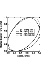
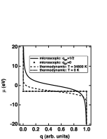
(a) (b)

Figure 3: (a) $\omega(q)$, corresponding to branches of the energy surfaces, Eq. (4), in the strong and intermediate limits for each root of the $\gamma-q$ relationship: $S_{\rm ci}=0.25$ and $\delta N_{\rm ci}^{*}=-0.20$ (strong); $S_{\rm ci}=0$ and $\delta N_{\rm ci}^{*}=0$ (intermediate). $q_{\rm gs}=0.25$ in both cases. Gaps form at integer charges. (b) Two-state microscopic and thermodynamic models of the chemical potential. The microscopic model is plotted for $q_{\rm gs}=0$ and $1/2$, and the thermodynamic model for $T=0$ and 34800 K.

Because there are no other degrees of freedom with which to equilibrate, it is clear that $T$ corresponds to an electronic temperature. In fact, this is the grand canonical (open system) analog of the electronic temperature introduced by Kohn KOH86 in the context of calculating excitation energies using closed system ensemble DFT OGK88 ; GOKII . The corresponding canonical ensemble is defined in terms of a spectral representation, as here, and is characterized by a temperature $\theta$. $\theta$ is defined implicitly through a self-consistent relation equating the total entropy of the system to the integrated local entropy of the system’s electron density distribution, in turn defined through a set of state- and temperature-dependent Kohn-Sham equations KOH86 ; OGK88 . There is thus a direct analogy between our electronic temperature for an open system with charge transfer, and that of Kohn et al., even though they restricted their attention to polarization excitations of a closed system with fixed total charge. In both treatments, the temperature corresponds to deviation of the charge distribution away from the ground state distribution. From a thermodynamic point of view, the excitations lead to an increase in entropy. The correspondence observed between $T$ and $q_{\rm gs}$ stems from the fact that both quantities encode information about the energetics of the microscopic states of the interacting subsystems. Equivalently, both $T$ and $q_{\rm gs}$ reflect the strength of the coupling between a subsystem and a reservoir.

In conclusion, we have shown how charge dependencies in a pair of subsystems can be described by appealing to an ensemble representation of the closed system energy, even in the strong interaction limit. The analytical form of the charge-dependent system energy is determined through a basis rotation involving the resonance states that embody charge transfer between subsystems. When a decomposition method is applied to closed system eigenenergies, charge-dependent, open system energies can be defined, leading to a microscopic model of the chemical potential. When the subsystems interact strongly, the derivative discontinuities in the energy found by PPLB move to noninteger charges that are outside of our physically allowed range, leading to continuous chemical potentials at the integer charges. When compared with a thermodynamic model of the chemical potential, a correlation is observed between the ground-state charge and an electronic temperature, thus defining complementary measures of the interaction strength.

The ensemble variational energy defined here may be regarded as the wavefunction predecessor of the excited-state density functionals of Gross et al. GOKII . However, the formal connection of our strongly-interacting, open system results to density functional theory remains an open question, requiring the construction of a variational principle for open system excited states. To the best of our knowledge such a variational principle has not yet been established.

The work of SMV was performed in part at Los Alamos National Laboratory under the auspices of the US Department of Energy, under contract No. W-7405-ENG-36, and funded through the Advanced Fuel Cycle Initiative. SMV thanks the University of New Mexico, Department of Physics and Astronomy for its hospitality during the 2003-2004 academic year. The authors thank the National Science Foundation for support of this work under grants DMR-9520371 (SRA) and CHE-0304710. SMV dedicates this work to his sister Susan.

References

- (1) See, e.g.: Th. Frauenheim, G. Seifert, M. Elstner, Z. Hajnal, G. Jungnickel, D. Porezag, S. Suhai, and R. Scholz, phys. stat. sol. (b) 217, 41 (2000).
- Rappé and Goddard (1991) A. K. Rappé and W. A. Goddard, III, J. Phys. Chem. 95, 3358 (1991).
- (3) J. P. Perdew, R. G. Parr, M. Levy, and J. L. Balduz, Jr., Phys. Rev. Lett. 49, 1691 (1982).
- (4) J. P. Perdew, in Density Functional Methods in Physics, NATO Advanced Science Institute Series, Vol. 123, edited by R. M. Dreizler and J. da Providência (Plenum Press, New York, 1984).
- (5) Y. Zhang and W. Yang, Theor. Chem. Acc. 103, 346 (2000).
- (6) J. Ciosłowski and B. B. Stefanov, J. Chem. Phys. 99, 5151 (1993).
- (7) R. G. Parr, P. W. Ayers, and R. F. Nalewajski, J. Phys. Chem. A 109, 3957 (2005).
- (8) Ph. Ghosez, J.-P. Michenaud, and X. Gonze, Phys. Rev. B 58, 6224 (1998).
- (9) W. A. Harrison, Electronic Structure and the Properties of Solids (Freeman, San Fransisco, 1980).
- (10) M. H. Cohen and A. Wasserman, Isr. J. Chem. 43 219 (2003).
- (11) Q. Wu and T. Van Voorhis, Phys. Rev. A 72, 024502 (2005).
- (12) S. M. Valone and S. R. Atlas, J. Chem. Phys. 120, 7262 (2004).
- Nalewajski (1998) R. F. Nalewajski, Int. J. Quant. Chem., 69, 591 (1998).
- (14) J. Morales and T. J. Martinez, J. Phys. Chem. A 105, 2842 (2001).
- (15) J. Morales and T. J. Martinez, J. Phys. Chem. A 108, 3076 (2004).
- (16) A. Warshel and A. Bromberg, J. Chem. Phys. 52, 1262 (1970); A. Warshel and R. M. Wiess, J. Am. Chem. Soc. 102, 6218 (1980); J. Åqvist and A. Warshel, Chem. Rev. 93, 2523 (1993).
- (17) R. S. Mulliken, Phys. Rev. 50, 1017 (1936); ibid., 50, 1028 (1936).
- (18) J. C. Phillips, Rev. Mod. Phys. 42, 317 (1970).
- (19) C. A. Coulson, L. B. Rèdei, and D. Stocker, Proc. Roy. Soc. (London) 270, 357 (1962).
- (20) S. A. Adelman and D. R. Herschbach, Molec. Phys. 33, 793 (1977).
- (21) “Strength” is defined through the energies of and overlaps between the charge resonances as defined in Ref. CT-EVB, : “Intermediate” means zero overlap but nonzero resonance energy. “Weak” means that both quantities are zero.
- (22) W. Yang, Y. Zhang, and P. W. Ayers, Phys. Rev. Lett. 84, 5172 (2000).
- (23) U. Fano, Rev. Mod. Phys. 29, 74 (1957).
- (24) X.-Y. Pan, V. Sahni, and L. Massa, Phys. Rev. Lett. 93, 130401 (2004).
- (25) R. T. Sanderson, Science 114, 670 (1951).
- (26) P. K. Chattaraj, A. Cedillo, and R. G. Parr, Chem. Phys. 204, 429 (1996).
- (27) P. W. Ayers, R. G. Parr, and A. Nagy, Int. J. Quant. Chem. 90, 309 (2002).
- (28) E. P. Gyftopoulos and G. N. Hastopoulos, Proc. Nat. Acad. Sci. USA 60, 786 (1968).
- (29) R. C. Tolman, The Principles of Statistical Mechanics (Dover, New York, 1979).
- (30) W. Kohn, Phys. Rev. A 34, 737 (1986).
- (31) L. N. Oliveira, E. K. U. Gross, and W. Kohn, Phys. Rev. A 37, 2821 (1988).
- (32) E. K. U. Gross, L. N. Oliveira, and W. Kohn, Phys. Rev. A 37, 2809 (1988).