Trapped Fermions across a Feshbach resonance with population imbalance

Abstract

We investigate the phase separation of resonantly interacting fermions in a trap with imbalanced spin populations, both at zero and at finite temperatures. We directly minimize the thermodynamical potential under the local density approximation instead of using the gap equation, as the latter may give unstable solutions. On the BEC side of the resonance, one may cross three different phases from the trap center to the edge; while on the BCS side or at resonance, typically only two phases show up. We compare our results with the recent experiment, and the agreement is remarkable.

The recent experimental realizations of condensation and superfluidity in Fermi gases near a Feshbach resonance have provided a new platform for controlled study of many-body physics in the strongly correlated region 1 . A significant advance in this direction is illustrated by two very recent experiments 2 ; 3 , which study the fermi superfluidity with controlled population imbalance of different spin components. With increasing population imbalance, a phase transition from the superfluid to the normal state has been observed 2 , and phase separation of the Fermi gas in the trap has been identified 2 ; 3 .

The Cooper pairing in the Fermi gas, which is essential for the Fermi condensate and the superfluidity, requires an equal number of atoms from both spin components. If the atomic gas has imbalanced population in its two spin states, inevitably some of the atoms will be unpaired, which triggers the competition between the Cooper pairing and the population imbalance. Such a competition may lead to various new phenomena 4 ; 5 ; 6 ; 7 ; 8 , which have raised strong interest recently 6 ; 7 ; 8 .

In this paper, we present our study on the trapped fermions across a Feshbach resonance with population imbalance. Compared with other recent theoretical works 6 ; 7 ; 8 , we demonstrate the following results: (i) We consider a wide resonance with parameters corresponding to the recent ${}^{6}Li$ experiment, and calculate the pairing gap and the density distribution, which can be directly compared with the experiment. (ii) We take into account the trapping potential, and show that the trap favors the phase separation, which is critical for the understanding of the recent experiments 2 ; 3 . Some of the co-existing or unstable phases in a homogeneous gas 8 necessarily become phase separated even if a very weak trap is turned on. (iii) We investigate the effect of the population imbalance both at zero and at finite temperatures. At zero temperature, the BCS superfluid state requires an equal number of atoms from both spin components; but at finite temperature $T$ it allows population imbalance carried by the quasiparticle excitations. This key difference significantly relaxes the competition between the population imbalance and the Cooper pairing at finite $T$, which helps to explain the robustness of the superfluid state in the recent experiment 2 . (iv) We directly minimize the thermodynamical potential to find out the stable configuration of the system, and caution the use of the gap equation in the case of population imbalance. In the region with competition between different phases, the gap equation often gives incorrect results or unstable solutions.

To describe the fermions across a Feshbach resonance, we take the following two-channel Hamiltonian 9 ; 10 ; 11 :

$$H = \sum_{\mathbf{k},\sigma}(\epsilon_{\mathbf{k}}-\mu_{\sigma})a_{\mathbf{k},\sigma}^{{\dagger}}a_{\mathbf{k},\sigma}$$

$$+ \sum_{\mathbf{q}}(\epsilon_{\mathbf{q}}/2+\gamma-\mu_{\uparrow}-\mu_{\downarrow})b_{\mathbf{q}}^{{\dagger}}b_{\mathbf{q}}$$

$$+ \alpha/\sqrt{\mathcal{V}}\sum_{\mathbf{q},\mathbf{k}}(b_{\mathbf{q}}^{{\dagger}}a_{\mathbf{q}/2-\mathbf{k},\downarrow}a_{\mathbf{q}/2+\mathbf{k},\uparrow}+h.c.),$$

$$+ U/\mathcal{V}\sum_{\mathbf{q},\mathbf{k},\mathbf{k^{\prime}}}a_{\mathbf{q}/2+\mathbf{k},\uparrow}^{{\dagger}}a_{\mathbf{q}/2-\mathbf{k},\downarrow}^{{\dagger}}a_{\mathbf{q}/2-\mathbf{k^{\prime}},\downarrow}a_{\mathbf{q}/2+\mathbf{k^{\prime}},\uparrow}$$

where $\epsilon_{\mathbf{k}}=k^{2}/(2m)$ ($m$ is the atom mass and $\hbar=1$), $\mu_{\sigma}$ is the chemical potential for the spin-$\sigma$ component ($\sigma=\uparrow,\downarrow$ labels the two spin states), $\mathcal{V}$ is the quantization volume, $a_{\mathbf{k},\sigma}^{{\dagger}}$ and $b_{\mathbf{q}}^{{\dagger}}$ are the creation operators for the fermionic atoms (open channel) and the bosonic molecules (closed channel), respectively. The bare atom-molecule coupling rate $\alpha$, the bare background scattering rate $U$, and the bare detuning $\gamma$ are connected with the physical ones $\alpha_{p},U_{p},\gamma_{p}$ through the standard renormalization relations 11 , and the values of $\alpha_{p},U_{p},\gamma_{p}$ are determined from the scattering parameters (see, e.g., the explicit expressions in Ref. 12 .). We take the local density approximation so that $\mu_{\uparrow}=\mu_{\mathbf{r}}+h,$ $\mu_{\downarrow}=\mu_{\mathbf{r}}-h$, $\mu_{\mathbf{r}}=\mu-V\left(\mathbf{r}\right)$, where $V\left(\mathbf{r}\right)$ is the external trap potential (slowly varying in $\mathbf{r}$), and $\mu,h$ are determined from the total atom number $N=N_{\uparrow}+N_{\downarrow}$ and the population imbalance $\beta=\left|N_{\uparrow}-N_{\downarrow}\right|/N$ through the number equations below.

For simplicity, we first take a mean-field approach by assuming $\langle b_{\mathbf{q}}\rangle=\langle b_{0}\rangle\delta_{\mathbf{q0}}=-\alpha/\sqrt{\mathcal{V}}\sum_{\mathbf{k}}\left\langle a_{-\mathbf{k},\downarrow}a_{\mathbf{k},\uparrow}\right\rangle/\left(\gamma-2\mu_{\mathbf{r}}\right)$ (the last equality comes from the Heisenberg equation for the operator $b_{\mathbf{q}}$). At this level, we neglect the pair/molecule fluctuation, an approximation that is valid near zero temperature or in the BCS limit. Later we will discuss how to incorporate the pair/molecule fluctuation directly into the final equations. We also neglect here the possibility of a non-zero-momentum pairing (the FFLO state 4 , with the pair momentum $\mathbf{q\neq}0$). This is motivated by the fact that the FFLO state is stable only within a narrow parameter window deep in the BCS region 8 and is absent in the recent ${}^{6}Li$ experiments 2 ; 3 .

With the mean-field approximation, one can then find out the thermodynamical potential $\Omega=-T\ln[$tr$\left(e^{-H/T}\right)]$ at temperature $T$ (the Boltzmann constant is taken to be $1$). It is given by the expression

$$\Omega=-\Delta^{2}\mathcal{V}/U_{T}-T\sum_{\mathbf{k}}\{\ln[1+\exp(-\left|E_{\mathbf{k}\downarrow}\right|/T)]\hskip 22.76228pt$$

$$+\ln[1+\exp(-E_{\mathbf{k}\uparrow}/T)]-[\epsilon_{\mathbf{k}}-\mu_{\downarrow}-\theta(E_{\mathbf{k}\downarrow})E_{\mathbf{k}\downarrow}]/T\},$$ (2)

where the parameter $U_{T}\equiv U-\alpha^{2}/\left(\gamma-2\mu_{\mathbf{r}}\right)$, the quasi-particle excitation energy $E_{\mathbf{k}\uparrow,\downarrow}=\sqrt{(\epsilon_{\mathbf{k}}-\mu_{\mathbf{r}})^{2}+\left|\Delta\right|^{2}}\mp h,$ and the gap $\Delta=\alpha\langle b_{0}\rangle/\sqrt{\mathcal{V}}+U/\mathcal{V}\sum_{\mathbf{k}}\langle a_{-\mathbf{k},\downarrow}a_{\mathbf{k},\uparrow}\rangle=z\langle b_{0}\rangle/\sqrt{\mathcal{V}}$ ($z\equiv\alpha-U\left(\gamma-2\mu_{\mathbf{r}}\right)/\alpha$). The $\theta$-function is defined as $\theta\left(x\right)=1$ for $x>0$ and $\theta\left(x\right)=0$ otherwise. Note that different from the equal-population case, the excitation energies $E_{\mathbf{k\sigma}}$ are different for the $\mathbf{\sigma=}\uparrow,\downarrow$ branches. Without loss of generality, we take $h<0$ so that $E_{\mathbf{k}\uparrow}>0$ always; while for a certain range of $h$, the sign of $E_{\mathbf{k}\downarrow}$ depends on the momentum $\mathbf{k}$ . When $E_{\mathbf{k}\downarrow}<0$, the atoms at that momentum are actually not paired (and thus have no contribution to $\Delta$) as pairing is energetically unfavorable (that is why we have $\left|E_{\mathbf{k}\downarrow}\right|$ and $\theta(E_{\mathbf{k}\downarrow})$ in Eq. (2)). This case corresponds to the so-called breached pair state 13 . From the variational condition $\partial\Omega/\partial\left|\Delta\right|^{2}=0$, we get the gap equation

$$\frac{1}{U_{Tp}}=-\frac{1}{\mathcal{V}}\sum_{\mathbf{k}}(\frac{1-f(E_{\mathbf{k}\uparrow})-f(E_{\mathbf{k}\downarrow})}{E_{\mathbf{k}\uparrow}+E_{\mathbf{k}\downarrow}}-\frac{1}{2\epsilon_{\mathbf{k}}}),$$ (3)

where the parameter $1/U_{Tp}\equiv 1/\left[U_{p}-\alpha_{p}^{2}/\left(\gamma_{p}-2\mu_{\mathbf{r}}\right)\right]=1/U_{T}+(1/\mathcal{V})\sum_{\mathbf{k}}\left[1/\left(2\epsilon_{\mathbf{k}}\right)\right]$ (the latter equality comes from the renormalization relation between $\gamma,\alpha,U$ and $\gamma_{p},\alpha_{p},U_{p}$ 11 ). From the relation $\partial\Omega/\partial\mu_{\sigma}=-n_{\mathbf{r}\sigma}\mathcal{V}$, where $n_{\mathbf{r}\sigma}$ is the density of the spin-$\sigma$ component, we get the number equations

$$n_{\mathbf{r}\sigma}=\frac{1}{\mathcal{V}}\sum_{\mathbf{k}}[u_{\mathbf{k}}^{2}f(E_{\mathbf{k},\sigma})+v_{\mathbf{k}}^{2}f(-E_{\mathbf{k},-\sigma})]+\frac{\left|\Delta\right|^{2}}{z^{2}},$$ (4)

where the parameters $u_{\mathbf{k}}^{2}=(E_{\mathbf{k}}+(\epsilon_{\mathbf{k}}-\mu_{\mathbf{r}}))/2E_{\mathbf{k}}$, $v_{\mathbf{k}}^{2}=(E_{\mathbf{k}}-(\epsilon_{\mathbf{k}}-\mu_{\mathbf{r}}))/2E_{\mathbf{k}}$, $E_{\mathbf{k}}=\sqrt{(\epsilon_{\mathbf{k}}-\mu_{\mathbf{r}})^{2}+\left|\Delta\right|^{2}}$, the fermi distribution $f(E)\equiv 1/\left(1+e^{E/T}\right)$, and we take $-\uparrow=\downarrow$ and vice versa. The last term $\left|\Delta\right|^{2}/z^{2}$ in $n_{\mathbf{r}\sigma}$ comes from the contribution of the molecule (closed-channel) population, which is small near a wide resonance. The atom densities $n_{\mathbf{r}\uparrow}$ and $n_{\mathbf{r}\downarrow}$ are connected with the total atom number and the population imbalance through $N=\int d^{3}\mathbf{r}\left(n_{\mathbf{r}\uparrow}+n_{\mathbf{r}\downarrow}\right)$, and $\beta=\int d^{3}\mathbf{r}\delta n_{\mathbf{r}}/N$ ($\delta n_{\mathbf{r}}\equiv n_{\mathbf{r}\downarrow}-n_{\mathbf{r}\uparrow}$).

The mean-field approach above neglects the pair/molecule fluctuation. With this fluctuation taken into account, there will be a non-condensed fraction of the pairs, which also contributes to the gap for the fermionic quasiparticles 11 . So the gap now is replaced by $\left|\Delta\right|^{2}=\left|\Delta_{s}\right|^{2}+\left|\Delta_{pg}\right|^{2}$, where $\left|\Delta_{s}\right|^{2}=z^{2}\left|\langle b_{0}\rangle\right|^{2}/\mathcal{V}$ and $\left|\Delta_{pg}\right|^{2}=z^{2}m_{nc}/\mathcal{V}$ 11 , with $\left|\langle b_{0}\rangle\right|^{2}$ and $m_{nc}$ representing the condensed and the non-condensed molecule numbers, respectively. With the interpretation of $\left|\Delta\right|$ as the total gap, the gap and the number equations above remain valid with the pair fluctuation (note that the contribution to $n_{\mathbf{r}\sigma}$ from the non-condensed molecules $m_{nc}$ is automatically taken into account by the last term in Eqs. (4)). If one wants to break up $\Delta$ to find out the superfluid order parameter $\Delta_{s}$ and the pseudogap $\Delta_{pg}$, one needs to know the dispersion relation for the pair/molecule excitations. Here, to compare with the experiments 2 ; 3 , we only calculate the total gap $\Delta$ and the atom density distributions $n_{\mathbf{r}\sigma}$. For that purpose, the above gap and number equations suffice, and we do not need to specify the pair dispersion relation. Note that the total gap $\Delta$ is the quantity directly measurable through the radio-frequency spectroscopy 15 .

The gap and the number equations above are in principle sufficient to determine the distribution of $\left|\Delta\right|$ and $n_{\mathbf{r}\sigma}$. However, different from the equal-population case, the solution of this set of equations turns out to be subtle, as they often give unstable phases or incorrect results. To understand this, we examine the behavior of the thermodynamical potential $\Omega$ under the variations of some system parameters. Note that the gap equation should give an optimal value of $\left|\Delta\right|$ which minimizes $\Omega$. However, with a population imbalance, the potential $\Omega$ has a double well structure in many cases. In  Fig. 1, we show $\Omega$ as a function of $\left|\Delta\right|$ as we change the chemical potential $\mu_{\mathbf{r}}$ (from the trap center to the edge), the potential difference $h$ (with varying population imbalance), the system temperature $T$, and the field detuning $\gamma_{p}$. One can see that the double-well structure shows up, in particular on the BCS side or in the low-temperature, large-imbalance cases. Typically, one minimum of the double-wells corresponds to $\left|\Delta\right|=0$ (the normal state) and the other has a nonzero $\left|\Delta\right|$. When $\Omega$ has a double-well structure, the gap equation can give an incorrect result in several different ways: first, it may pick up a solution corresponding to the maximum of $\Omega$ (the gap equation is satisfied at that point), which is obviously not stable; second, it can choose the shallow well, which gives a metastable but not the optimal configuration; and finally, the gap equation (3) is usually not satisfied with $\left|\Delta\right|=0$ even if the latter is the minimum of $\Omega$ (as $\partial\Omega/\partial\left|\Delta\right|^{2}\neq 0$ at that point). In this case, the numerical program gives an incorrect result in an uncontrollable way.

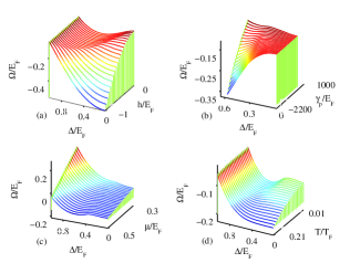
Figure 1: The thermodynamical potential $\Omega$ as a function of the total gap $|\Delta|$ with varying (a) $h$ (the chemical potential difference), (b) $\gamma_{p}$ (the field detuning), (c) $\mu$ (the chemical potential), and (d) $T$ (the temperature). We have used $T_{F}=E_{F}=k_{F}^{2}/2m$ as the unit of energy/tempeature, where $k_{F}=(3\pi^{2}n_{0})^{1/3}$ is a convenient inverse length scale corresponding to a density $n_{0}=3\times 10^{13}cm^{-3}$, typical for the ${}^{6}Li$ experiments. The parameters $\alpha_{p},U_{p}$ take the standard values for the ${}^{6}Li$ atoms with $\alpha_{p}\sqrt{n_{0}}=-0.6E_{F}$, and $U_{p}n_{0}=-82E_{F}$. The other parameters for Figs. (a-d) are given by (a)$\mu=0.5E_{F}$, $\gamma=0$, $T=0.01T_{F}$; (b) $\mu=0.5E_{F}$, $h=-0.35E_{F}$, $T=0.01T_{F}$; (c) $h=-0.35E_{F}$, $\gamma=0$, $T=0.01T_{F}$; and (d) $\mu=0.5E_{F}$, $h=-0.35E_{F}$, $\gamma=0$.

To overcome the above problems, we always check the stability of the solution by finding out all the minima of the thermodynamical potential $\Omega$. Note that although the metastable state at the bottom of a shallow well of $\Omega$ does not give the ground state configuration, it has a finite relaxation time and may appear in real experiments under certain circumstances (similar to the superheating or supercooling phenomena in a classical phase transition). So, in that sense, the state of the system may not be unique. To avoid this complexity, in the following we assume the system to be in its equilibrium configuration by choosing the solution corresponding to the global minimum of the thermodynamical potential $\Omega$.

Through minimization of the thermodynamical potential, we have calculated the gap and the density distributions for trapped fermions with different magnetic field detunings, at both zero and finite temperatures. Fig. 2 shows some typical results. To summarize, we find that the gas is separated into several different phases from the trap center to the edge, with the number of phases and their boundary sensitive to the detuning $\gamma_{p}$, the population imbalance $\beta$, and the temperature $T$. At zero temperature and on the BEC side of the resonance with a small population imbalance, there are typically three different phases: the superfluid phase occupies the center of the trap, where all the particles are paired with no population imbalance (the SF phase). Further out from the center, when the pairing gap becomes smaller than the chemical potential difference $\left|h\right|$, there is a second phase, in which the particles are paired except for a finite region of the momentum shell (the breached pair phase 6 , or in short, the BP phase). This BP phase is characterized by a nonzero $\left|\Delta\right|$, but with excessive fermions in the breached momentum shell, which gives a finite population imbalance. In Fig. 2(a), the middle region with $\left|\Delta\right|$ and $\delta n_{\mathbf{r}}$ both nonzero corresponds to such a phase. Towards the edge of the trap, where the pairing gap has already vanished, only the normal Fermi sea is left, with different Fermi surfaces for different spin components. As the population imbalance increases, the SF phase at the center of the trap depletes and yields to the surrounding BP phase and the normal Fermi sea. At the resonance or further out to the BCS side, this picture is different in that there are now only two stable phases, the SF phase and the normal phase, as shown in Fig. 2(b) (the BP phase in the middle loses its stability). As the population imbalance increases and reaches a critical value, the system undergoes a SF-normal phase transition, and the trap is left with only the normal Fermi gas.

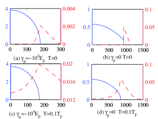
Figure 2: The gap ($|\Delta|$) and the differential density ($\left|\Delta\right|$ and $\delta n_{\mathbf{r}}$) distributions for the trapped fermions, both at zero and at finite temperature. The $x$-axis is the distance from the trap center, in the unit of $k_{F}r$. The solid curves represent $|\Delta|$ (the left $y$-axis) and the dashed ones are for $\delta n_{\mathbf{r}}$ ( the right $y$-axis). The other parameters are given by (a)(c)$\mu=-111.48E_{F}$, $h=-111.52E_{F}$; and (b)(d) $\mu=0.5E_{F}$, $h=-0.1E_{F}$. The corresponding population imbalance ratio $\beta$ and the total atom number $N$ are (a) $1\%$, $3.1\times 10^{5}$; (b) $6\%$, $3.9\times 10^{7}$; (c) $69\%$, $7.9\times 10^{5}$; and (d) $17\%$, $4.0\times 10^{7}$, respectively.

At finite temperature, the main difference is that there are fermionic excitations in the SF phase, which carry population imbalance of the spin components. As a result, it becomes easier to satisfy the population imbalance constraint, as with a fixed imbalance ratio $\beta$, the corresponding chemical potential difference $\left|h\right|$ becomes significantly smaller. This helps to stabilize the SF phase in the case of imbalanced population. Because of this feature, we cannot use $\delta n_{\mathbf{r}}$ to distinguish the SF and the BP phases any more, so the boundary between them becomes obscure. The population difference $\delta n_{\mathbf{r}}$ is peaked at the point where the gap $\left|\Delta\right|$ vanishes, marking the only distinguishable phase separation between the paired phase (SF or BP) and the normal phase (see Fig. 3c and 3d). At higher temperatures, the paired phase in the trap shrinks and finally disappears at the pair disassociation temperature $T^{\ast}$ (the superfluidity should disappear before that with $T_{c}<T^{\ast}$ 11 ). In Fig. 2(c) and (d), we show the distribution of $\left|\Delta\right|$ and $\delta n_{\mathbf{r}}$ at a typical temperature of $0.1E_{F}$, for the BEC and the resonance-BCS sides, respectively.

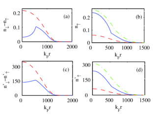
Figure 3: The atom density distributions in a trap, calculated with parameters corresponding to the recent MIT experiment 2 with $T\sim 0.1E_{F}$, and $\gamma\sim 2100E_{F}$ ($B-B_{0}\sim 56.3G$). The solid, the dashed, and the dash-dot curves correspond to the imbalance ratio $\beta\sim 46\%$ (the corresponding $\mu=0.5E_{F}$, $h=-0.12E_{F}$), $\beta\sim 86\%$ (the corresponding $\mu=0.43E_{F}$, $h=-0.23E_{F}$), and $\beta=0$ ($\mu=0.5E_{F}$, $h=0$) respectively, with the total atom number $N\sim 2.7\times 10^{7}$ in all the cases. Figs. (c,d) show the column integrated density distributions corresponding to Figs. (a,b).

Finally, to compare with the recent MIT experiment 2 , we calculate the density distributions $n_{\mathbf{r}\sigma}$, with all the parameters roughly the same as those in the experiment (the experimental temperature may have some uncertainties). The results are plotted in Fig. 3. It shows a pretty good agreement with the experimental data (Fig. 3 of Ref. 2 ), at least semi-quantitatively. In particular, the calculation shows that the distribution $\delta n_{\mathbf{r}}$ has a dip at the trap center with a moderate population imbalance ($\beta=46\%$); while the dip disappears when $\beta$ becomes large ($86\%$), which agrees exactly with the experimental findings.

In summary, we have studied the effects of trap and temperature on fermions across a wide Feshbach resonance with population imbalance. We propose to directly minimize the thermodynamical potential in order to overcome the instability problem associated with the solution of the gap equation. We establish a general phase separation picture for the trapped fermions across the whole resonance region, at both zero and finite temperatures. We have also compared our calculation with a recent experiment, and recovered some of the main experimental findings.

Note added: Upon completion of this work, two preprints [P. Pieri, G.C. Strinati, cond-mat/0512354; J. Kinnunen, L.M. Jensen, P. Torma, cond-mat/0512556] appeared on arxiv, where a similar problem are investigated at zero temperature with different theoretical approaches.

We thank Jason Ho, Martin Zwierlein, Wolfgang Ketterle, and Kathy Levin for helpful discussions. This work was supported by the NSF award (0431476), the ARDA under ARO contracts, and the A. P. Sloan Foundation.

References

- (1) C.A. Regal, M. Greiner and D.S. Jin, Phys. Rev. Lett. 92, 040403 (2004); M.W. Zwierlein et al., Phys. Rev. Lett. 92, 120403 (2004); M.W. Zwierlein et al., Nature 435, 1047 (2005).
- (2) M.W. Zwierlein, A. Schirotzek, C.H. Schunck, and W. Ketterle, Science 311, 492 (2006).
- (3) G.B. Partridge, W. Li, R.I. Kamar, Y. Liao, and R.G. Hulet, Science 311, 503 (2006).
- (4) P. Fulde and R. A. Ferrell, Phys. Rev. 135, A550 (1964); A.I. Larkin and Y.N. Ovchinnikov, Sov. Phys. JETP 20, 762 (1965).
- (5) G. Sarma, J. Phys. Chem. Solids 24, 1029 (1963).
- (6) W.V. Liu and F. Wilczek, Phys. Rev. Lett. 90, 047002 (2003); M. M. Forbes et al., Phys.Rev.Lett. 94, 017001 (2005).
- (7) R. Combescot, Europhys. Lett. 55, 150 (2001); P. F. Bedaque, H. Caldas, and G. Rupak, Phys. Rev. Lett. 91, 247002 (2003); H. Caldas, Phys. Rev. A 69, 063602 (2004); A. Sedrakian et al. Phys. Rev. A 72, 013613 (2005); T. D. Cohen, Phys. Rev. Lett. 95, 120403 (2005); J. Carlson and S. Reddy, Phys. Rev. Lett. 95, 060401 (2005); T. Mizushima, K. Machida, and M. Ichioka, Phys. Rev. Lett. 94, 060404 (2005); P. Castorina et al., Phys. Rev. A 72, 025601 (2005). D.T. Son and M.A. Stephanov, cond-mat/0507586.
- (8) D.E. Sheehy and L. Radzihovsky, cond-mat/0508430; C.-H. Pao, S.-T. Wu, and S.-K. Yip, cond-mat/0506437.
- (9) M. Holland et al., Phys. Rev. Lett. 87, 120406 (2001); Y. Ohashi and A. Griffin, Phys. Rev. Lett. 89, 130402 (2002).
- (10) E. Timmermans, et al., Phys. Rep. 315, 199 (1999).
- (11) Q.J. Chen, et al., Phys. Rep. 412, 1 (2005).
- (12) L.-M. Duan, Phys. Rev. Lett. 95, 243202 (2005).
- (13) This phase has various names in the literature, see Refs. 6 ; 5 ; 8 . We follow the terminology of Ref. 6 .
- (14) P. Pieri, G.C. Strinati, Phys. Rev. B 71, 094520 (2005).
- (15) C. Chin et al., Science 305, 1128 (2004); J. Kinnunen, M. Rodriguez, P. Torma, Science 305, 1131 (2004).