Theory of matter wave beam splitters in gravito-inertial and trapping potentials

Abstract

We present a strong field theory of matter wave splitting in the presence of various gravitational, inertial and trapping potentials. The effect of these potentials on the resonance condition (between the splitting potential and the considered effective two-level system) and on the atomic Borrmann effect is investigated in detail. The dispersive structuring of an incident atomic wave packet - due to such generalized beam splitters - is studied and modeled, and several important dynamical features of the solutions are detailed (generalized Rabi oscillations, velocity selection, anomalous dispersion, generalized Borrmann effect and anomalous gravitational bending). Finally, we show how to express this triple interaction “matter - splitting potential - gravito-inertial and trapping potentials” as an equivalent instantaneous interaction which turns out to be a very efficient tool for the modeling of atom interferometers.

PACS number(s): 03.75.-b, 32.80.-t, 33.80.-b, 39.25.+k, 42.50.-p

1 Introduction

The matter wave beam splitters are nowadays the cornerstone of a wide range of experiments, from atomic clocks and gravito-inertial sensors to laser cooling and ultracold atoms characterization, quantum computing and cavity QED experiments, atom lithography and chemical reaction dynamics, detection of tiny effects of General Relativity and test of fundamental theories, measurement of atom surface interactions…

In view of the recent progress in non-dissipative atom optics (coherent beam splitters, mirrors, lenses…) as well as in dissipative atom optics (slowing, trapping and cooling of atoms and molecules), it is needed to deepen our comprehension of light-matter interactions in the presence of other external potentials, like gravito-inertial or trapping potentials. In particular, the precision and stability of atom interferometers are now so outstanding [1] that it is necessary to go beyond the former modeling of their main component, namely the beam splitters.

In fact, the concept of atomic beam splitter is not confined to light-matter interactions, and can be extended to any interaction process between matter waves. It is thus possible to write the action of such atom optical elements as a S matrix between the incident and diffused matter waves, where the S matrix depends mainly on the “splitting” potential, which can be material (slits, periodic microstructures…) or electromagnetic (magnetic or electric static fields, laser fields…). This S matrix description is particularly useful for the modeling of atom interferometers, and more generally for any set up having a succession of such beam splitters [2, 3, 4].

However, for a long time, the precision of atom optics experiments has remained low enough not to require an accurate study of matter wave beam splitters. Thus, in the most common simplified modeling of these elements, only the following effects were considered: 1) the splitting of an incident atomic wave packet into several wave packets, 2) among them one was equal to the incident wave packet, up to a change of amplitude, 3) and where the others could differ from the incident wave packet in their central momentum, internal state, amplitude and phase. However, this practical modeling - sometimes called “infinitely thin” because it amounts to neglecting the duration of the interaction - does not take into account several important effects, like the dispersive structuring of the incident wave packet (velocity selection and sidebands, Borrmann effect, anomalous dispersion…), the time and space dependency of the splitting potential, the effect of relaxation processes, or the effect of other external fields during the splitting (time-dependent gravito-inertial effects, trapping potentials…).

During the last past two decades, several authors studied some of these problems, namely: the effect of a non-trivial time dependency of the splitting potential (for running and standing laser beam splitters) [5, 6, 7, 8, 9]; the atomic Borrmann effect and anomalous dispersion effect without any other external potential [10, 11] or with a constant and uniform acceleration (WKB solution [12]); the atomic splitting in a constant and uniform acceleration (exact solution in the temporal case and WKB solution in the spatial case) [13]; a common modeling for both spatial and temporal beam splitters to the first order in the splitting potential (weak field theory) [14]…

In the light of what happened in neutron optics, where the beam splitters modeling proved to be crucial to understand properly the origin of the interferometer phase shifts [15, 16], it appears to be necessary to go beyond these studies, so as to provide a comprehensive modeling of the true action of a matter wave beam splitter (strong fields theory for all the involved external fields).

This paper is organized as follows. First, we give some details on our framework and explain how to put in equation the problem of the triple interaction “matter - splitting potential - other external fields”. Then, we detail how to transform the obtained equation in a simpler one thanks to unitary transformations (interaction picture) and passage into the rotating frames. We expound then how to solve this equation (analytically or numerically, with different developments or relevant approximations), and we go back to the initial representation to explain how to write the effect of such beam splitters as an effective instantaneous interaction (generalized $ttt$ scheme). Finally, we study the atomic Borrmann effect and other anomalous dispersive properties and model them in the general framework detailed in the second part.

2 Framework and approximations

2.1 General framework

The matter wave beam splitters we consider in this paper consist of multi-level atomic systems subject to an interaction potential which couples the levels together. This interaction is usually made in the presence of other external potentials and miscellaneous relaxation processes.

In fact, these “atomic systems” can refer to atoms (neutral or not) as well as molecules, and more generally to any quantity of matter which can be coherently manipulated.

Furthermore, the atomic levels are not restricted to internal atomic levels, but more generally refer to energy-momentum states (i.e. eigenstates of both the internal and kinetic Hamiltonians). The transitions can occur between internal states only (spectroscopy without Doppler effect for example), external states only (diffraction in Kapitza-Dirac and Bragg regimes, optical Stern-Gerlach effect, magnetic atom mirror…), or between entangled states, where the entanglement may be between the internal and external states (stimulated Raman transitions for example) or between the previous energy-momentum states and the eigenstates of the interaction potential (Fock states of the quantized electromagnetic field for example).

There are many techniques to coherently split a matter wave, and each of them corresponds to a particular kind of splitting potential. Like the other atom optics elements, matter wave beam splitters use essentially two properties of atoms (or molecules): their wave property, and their interaction with external fields, electromagnetic or material. To date, the demonstrated matter wave beam splitters are based on:

1. atom-matter interaction: front wave division (material slits) [17], amplitude splitting (transmission material gratings) [18], reflection at crystalline surface [19], quantum reflection [20]…

2. interaction with static magnetic or electric fields (for atoms having a dipolar electric or magnetic moment): longitudinal Stark effect [21], transverse and longitudinal Stern-Gerlach effects [22], magnetic mirrors [23], mirror for polar molecules [24], Y shaped magnetic guides [25]…

3. resonant or quasi-resonant interaction with laser fields: reflection and diffraction by standing [26], running [27, 28] or evanescent [29] laser waves (with spatial and/or temporal working), optical Stern-Gerlach effect [30], stimulated Raman effect [28] and its derivatives (adiabatic transfer [31], STIRAP [32], CHIRAP [33]…), magneto-optical beam splitters [34], X shaped dipolar guides [35]…

In this paper, we will focus on this third kind of interaction, and more generally on the beam splitters for which the two-beam approximation is valid.

As for the relaxation processes, they refer to all the processes which lead to a loss of coherence and/or a loss of atoms (spontaneous emission, inter-atomic collisions, absorption and interaction with the material microstructures…). When they can not be neglected, the use of a density operator formalism is needed.

Other external potentials may be present during the matter wave splitting: inertial and gravitational fields, trapping potential, van der Waals and Casimir potentials… In this paper, we consider all the time-dependent potentials which are at most quadratic in position and momentum. The corresponding Hamiltonian is therefore:

$$H_{ext}=\frac{1}{2m}\overrightarrow{p}.\overset{\Rightarrow}{\beta}\left(t\right).\overrightarrow{p}-\frac{m}{2}\overrightarrow{r}.\overset{\Rightarrow}{\gamma}\left(t\right).\overrightarrow{r}-\overrightarrow{r}.\overset{\Rightarrow}{\alpha}\left(t\right).\overrightarrow{p}-m\overrightarrow{g}\left(t\right).\overrightarrow{r}+\overrightarrow{f}\left(t\right).\overrightarrow{p}$$

This includes the effect of non-uniform accelerations ($\overrightarrow{g}\left(t\right)$ and $\overset{\Rightarrow}{\gamma}\left(t\right)$), rotations (with an angular velocity $\overrightarrow{\Omega}\left(t\right)$ such that $\overset{\Rightarrow}{\alpha}\left(t\right).\overrightarrow{u}:=-\overrightarrow{\Omega}\left(t\right)\times\overrightarrow{u}$ for any vector $\overrightarrow{u}$), trapping potentials ($-$ $\overset{\Rightarrow}{\gamma}\left(t\right)$), non-zero curvature tensor ($\overset{\Rightarrow}{\gamma}\left(t\right)$), gravitational waves in Fermi’s gauge ($\overset{\Rightarrow}{\gamma}\left(t\right)$) or Einstein’s gauge ($\overset{\Rightarrow}{\beta}\left(t\right)$), and all the electromagnetic potentials which can be written as a development at most quadratic in position and momentum ($\overrightarrow{g}\left(t\right)$, $\overset{\Rightarrow}{\gamma}\left(t\right)$, $\overrightarrow{f}\left(t\right)$). Furthermore, to keep an overall approach, the coefficients of $H_{ext}$ are time-dependent, and $\overset{\Rightarrow}{\alpha}$, $\overset{\Rightarrow}{\beta}$ and $\overset{\Rightarrow}{\gamma}$ are expressed with non-diagonal 3x3 matrices.

2.2 Approximations considered in this paper

It is often possible to simplify this general framework and obtain an evolution equation between only two effective states by using some justified approximations.

First, the two-beam approximation is indeed valid when only two energy-momentum eigenstates are coupled. The coupling can be direct (for true two-level systems) or indirect (Raman transitions, spatial beam splitters in Bragg regime). In fact, one can show that any N-photon transition (thanks to several running or standing laser waves) of a multilevel atom is equivalent to an effective 1-photon transition between two atomic levels if the other levels can be adiabatically eliminated [36, 37]. The effective photon may not be real. For example, in the Bragg regime, the wave vector of this effective photon is equal to $N\hbar\overrightarrow{k}$ and its frequency is equal to $0$. Eventually, the spatial and temporal structure of the true laser beams appears only in the amplitude of the effective running laser beam.

Second, the laser fields are considered as classical (coherent states of the quantized electromagnetic fields), but the calculations which follow are also valid for a transition between two dressed states [38].

Third, we suppose that the two atomic levels have a long lifetime and we neglect all the relaxation processes listed before. However, the instability of these levels, due to spontaneous emission, can be taken into account in an approximative manner adding a non-Hermitian part to the atom-laser Hamitonian $V_{em}$ [38].

In addition, $V_{em}$ is chosen equal to the usual dipolar electric Hamiltonian (without spin) and we suppose that the other external fields are sufficiently weak to neglect their effect on the atomic levels and laser fields.

Finally, the triple interaction “laser - matter - other external fields” can be written as a Schrödinger equation concerning two atomic states coupled by an effective running laser wave:

$$i\hbar\frac{d}{dt}\left|\Psi\left(t\right)\right\rangle=\left(H_{0}+H_{ext}\left(\overrightarrow{r_{op}},\overrightarrow{p_{op}},t\right)+V_{em}\left(\overrightarrow{r_{op}},t\right)\right)\left|\Psi\left(t\right)\right\rangle$$ (1)

where $\overrightarrow{r_{op}}$ and $\overrightarrow{r_{op}}$ are the position and momentum operators, and $H_{0}$ the internal Hamiltonian ($E_{b}>E_{a}$):

$$H_{0}=\left(\begin{array}[c]{cc}E_{b}&0\\ 0&E_{a}\end{array}\right)=\frac{E_{a}+E_{b}}{2}1+\frac{\hbar\omega_{0}}{2}\sigma_{3}$$

where $\omega_{0}=\left(E_{b}-E_{a}\right)/\hbar$ is the atomic transition frequency and $\sigma_{3}$ the usual third Pauli matrix.

It is also possible to account for some relativistic effects by introducing two different masses [14, 4]. For simplicity however, we will not take into account these relativitic corrections and use only one atomic mass in what follows.

3 Interaction picture and rotating frames

It is generally impossible to solve directly the equation (1) (non-trivial time dependence of the right hand side, presence of two non-commuting operators $\overrightarrow{r_{op}}$ and $\overrightarrow{r_{op}}$), but it is possible to simplify it with the help of well chosen unitary transformations [4].

The main idea of this series of transformations is to eliminate progressively the different sources of evolution (internal and external) of the right hand side of (1). As each unitary transformation corresponds to a change of frame, we can see this succession of transformations as a succession of frame changes which aims at reaching the proper frame of the atom, or, at least, at reaching a “least movement frame” for the atom (from external as well as internal points of view). In this especially suitable frame, it is easier to solve the evolution equation and several important pieces of information about the solution can be directly seen.

First, let us go to the interaction picture with respect to $H_{0}$ and$\ H_{ext}$:

$$\left|\Psi\left(t\right)\right\rangle=U_{1}\left(t,t_{1}\right)\left|\varphi_{1}\left(t\right)\right\rangle$$ (2)

with :

$$U_{1}\left(t,t_{1}\right)=e^{-\frac{i}{\hbar}H_{0}.\left(t-t_{1}\right)}U_{ext}\left(t,t_{1}\right)$$

and:

$$U_{ext}\left(t,t_{1}\right)=\mathcal{T}\left(\exp\left(-\frac{i}{\hbar}\int_{t_{1}}^{t}H_{ext}\left(\overrightarrow{r_{op}},\overrightarrow{p_{op}},t^{\prime}\right)dt^{\prime}\right)\right)$$

where $\mathcal{T}$  is the chronological Dyson operator and $t_{1}$ an arbitrary time (different from $t$ by definition).

The equation (1) becomes:

$$i\hbar\frac{d}{dt}\left|\varphi_{1}\left(t\right)\right\rangle=e^{\frac{i}{\hbar}H_{0}.\left(t-t_{1}\right)}V_{em}\left(\overrightarrow{R_{op}}\left(t,t_{1}\right),t\right)e^{-\frac{i}{\hbar}H_{0}.\left(t-t_{1}\right)}\left|\varphi_{1}\left(t\right)\right\rangle$$ (3)

where $\overrightarrow{R_{op}}$ is defined as:

$$\overrightarrow{R_{op}}\left(t,t_{1}\right)=U_{ext}\left(t,t_{1}\right)^{-1}\text{ }\overrightarrow{r_{op}}\text{ }U_{ext}\left(t,t_{1}\right)$$

The external Hamiltonian $H_{ext}$ being at most quadratic in position and momentum, $\overrightarrow{R_{op}}$ depends linearly on $\overrightarrow{r_{op}}$ and $\overrightarrow{p_{op}}$:

$$\overrightarrow{R_{op}}\left(t,t_{1}\right)=A\left(t,t_{1}\right)\text{ }\overrightarrow{r_{op}}+B\left(t,t_{1}\right)\text{ }\overrightarrow{p_{op}}/m+\overrightarrow{\xi}\left(t,t_{1}\right)$$

and is simply obtained through the classical solution of the Hamilton’s equations. One can show that the matrices $A$ and $B$ depend on the quadratic terms of $H_{ext}$ ($\overset{\Rightarrow}{\alpha}\left(t\right)$, $\overset{\Rightarrow}{\beta}\left(t\right)$ and $\overset{\Rightarrow}{\gamma}\left(t\right)$) only, whereas $\overrightarrow{\xi}\left(t,t_{1}\right)$ also depends on its linear terms ($\overrightarrow{g}\left(t\right)$ and $\overrightarrow{f}\left(t\right)$). These matrices are in fact the well known $ABCD$ matrices, usually used in Gaussian optics, and introduced recently in atom optics [39, 4].

As far as $V_{em}$ is concerned, it may have diagonal terms (AC stark shifts, slowly varying in space and time). However, in a first approach, we can take the latter constant and eliminate their common part by a unitary transformation. Finally, $V_{em}$ can be taken as purely anti-diagonal:

$$V_{em}\left(\overrightarrow{r_{op}},t\right)=V\left(\overrightarrow{r_{op}},t\right)\left(\begin{array}[c]{cc}0&1\\ 1&0\end{array}\right)$$

with:

$$V\left(\overrightarrow{r},t\right)=-2\hbar\Omega_{0}F\left(\overrightarrow{r},t\right)\cos\left(\omega t-\overrightarrow{k}.\overrightarrow{r}+\phi\right)$$

where $F\left(\overrightarrow{r},t\right)$ is the amplitude of the effective running laser beam, and where $\Omega_{0}$ is the Rabi frequency of the atomic transition.

An other important approximation is the rotating wave approximation (RWA), which consists in neglecting the off-resonant terms (i.e. with frequency $\omega+\omega_{0}$) in (3). In our case, this approximation is supposed to be justified. Indeed, if the two effective levels are indirectly coupled through optical photons (as for Raman transitions for example), one can show that the Bloch-Siegert effect is negligible [40].

Finally, the evolution equation is equal to:

$$\frac{d}{dt}\left|\varphi_{1}\left(t\right)\right\rangle=i\Omega_{0}F\left(\overrightarrow{R_{op}}\left(t,t_{1}\right),t\right)\left(\begin{array}[c]{cc}0&e^{-i\Phi_{op}\left(t,t_{1}\right)}\\ e^{+i\Phi_{op}\left(t,t_{1}\right)}&0\end{array}\right)\left|\varphi_{1}\left(t\right)\right\rangle$$

where $\Phi_{op}$ is defined as:

$$\Phi_{op}\left(t,t_{1}\right)=\omega t-\omega_{0}\left(t-t_{1}\right)-\overrightarrow{k}.\overrightarrow{R_{op}}\left(t,t_{1}\right)+\phi$$

The next unitary transformation corresponds to the usual passage into the rotating frame. In fact, there is an infinity of such transformations [4]. For example, the following family of transformations (indexed by the real parameter $x$):

$$\left|\varphi_{1}\left(t\right)\right\rangle=U_{2}\left(x,t,t_{1}\right)\left|\varphi_{2}\left(x,t\right)\right\rangle$$ (4)

with:

$$U_{2}\left(x,t,t_{1}\right)=\left(\begin{array}[c]{cc}e^{-i\Phi_{op}\left(t,t_{1}\right).x}&0\\ 0&e^{-i\Phi_{op}\left(t,t_{1}\right).\left(x-1\right)}\end{array}\right)$$

leads to the equation:

$$\framebox{$\frac{d}{dt}\left|\varphi_{2}\left(x,t\right)\right\rangle=iM_{op}\left(x,t\right)\left|\varphi_{2}\left(x,t\right)\right\rangle$}$$ (5)

with $M_{op}$ defined as:

$$M_{op}\left(x,t\right)=\left(\begin{array}[c]{cc}x\left(\omega-\omega_{0}-\overrightarrow{k}.\overset{\cdot}{\overrightarrow{R_{op}}}-x\delta\right)&\Omega_{0}F_{op}\\ \Omega_{0}F_{op}&\left(x-1\right)\left(\omega-\omega_{0}-\overrightarrow{k}.\overset{\cdot}{\overrightarrow{R_{op}}}-\left(x-1\right)\delta\right)\end{array}\right)$$

where $\delta\left(t,t_{1}\right)$ is the “generalized recoil”:

$$\delta\left(t,t_{1}\right)=\hbar\overrightarrow{k}\beta\overrightarrow{k}/2m$$

and where the point above letters refers to the time derivative.

Each value of $x$ corresponds to a particular evolution equation. For example, the most “symmetric” choice is $x=1/2$, whereas the most “physical” choice is $x=1$, and leads to:

$$M_{op}\left(1,t\right)=\left(\begin{array}[c]{cc}\Delta_{op1}&\Omega_{0}F_{op}\\ \Omega_{0}F_{op}&0\end{array}\right)$$

where $\Delta_{op1}$ is the “generalized detuning” [4]:

$$\Delta_{op1}\left(t,t_{1}\right)=\omega-\omega_{0}-\overrightarrow{k}.\overset{\cdot}{\overrightarrow{R_{op}}}-\delta$$

i.e., the operator which generalizes the usual “free” detuning in the presence of several gravitational, inertial and trapping potentials. It can also be written as:

$$\Delta_{op1}\left(t,t_{1}\right)=\omega-\left(\omega_{0}+\overrightarrow{k}\left[\frac{\beta}{m}\left(\overrightarrow{P_{op}}+\frac{\hbar\overrightarrow{k}}{2}\right)+\alpha\overrightarrow{R_{op}}+\overrightarrow{f}\right]\right)$$

where $\overrightarrow{P_{op}}$ is defined in the same way as $\overrightarrow{R_{op}}$ [3, 4]:

$$\overrightarrow{P_{op}}\left(t,t_{1}\right)/m=C\left(t,t_{1}\right)\text{ }\overrightarrow{r_{op}}+D\left(t,t_{1}\right)\text{ }\overrightarrow{p_{op}}/m+\overrightarrow{\phi}\left(t,t_{1}\right)$$

The expression of $\Delta_{op1}\left(t,t_{1}\right)$ can be easily interpreted considering the energy-momentum conservation for a non-excited atom absorbing a photon ($\omega$, $\overrightarrow{k}$) at the instant $t$ (the considered atom is then at the position $\overrightarrow{R}\left(t,t_{0}\right)$ with the momentum $\overrightarrow{P}\left(t,t_{0}\right)$ when the absorption occurs):

$$H_{ext}\left(\overrightarrow{R}\left(t,t_{0}\right),\overrightarrow{P}\left(t,t_{0}\right),t\right)+E_{b}+\hbar\omega\text{ }=\text{ }H_{ext}\left(\overrightarrow{R}\left(t,t_{0}\right),\overrightarrow{P}\left(t,t_{0}\right)+\hbar\overrightarrow{k},t\right)+E_{a}$$

which gives the non-operatorial version of the condition $\Delta_{op1}\left(t,t_{1}\right)=0$ (exact resonance condition in the presence of the external potentials described by $H_{ext}$).

This generalized detuning can also be expressed directly with the coefficients of $H_{ext}$. For example, if $H_{ext}$ is constant, the first terms of its Taylor expansion (in $\alpha(t-t_{1})$ and $\gamma(t-t_{1})^{2}$) are found to be [4]:

$$\Delta_{op1}\left(t,t_{1}\right) =\omega-\omega_{0}-\overrightarrow{k}.\frac{\overrightarrow{p_{op}}}{m}-\delta-\overrightarrow{k}.\overrightarrow{g}\left(t-t_{1}\right)-\overrightarrow{k}.\alpha.\overrightarrow{r_{op}}$$ (6)

$$-2\overrightarrow{k}.\alpha.\frac{\overrightarrow{p_{op}}}{m}\left(t-t_{1}\right)-\overrightarrow{k}.\left(\alpha^{2}+\gamma\right).\overrightarrow{r_{op}}\left(t-t_{1}\right)-\overrightarrow{k}.\alpha.\overrightarrow{g}\left(t-t_{1}\right)^{2}-...$$

where only the first five terms of the right hand side are non-negligible in usual experiments (weak rotations and acceleration gradients on the Earth). We can then use chirped laser pulses to eliminate the gravitational induced Doppler shift $\overrightarrow{k}.\overrightarrow{g}\left(t-t_{1}\right)$ and finally get back the usual “free” detuning.

The other element of $M_{op}\left(x,t\right)$ which may depend on the two canonical operators is the effective amplitude $F\left(\overrightarrow{R_{op}}\left(t,t_{1}\right),t\right)$. The two main sources of its spatial dependency are its transverse profile and the speckle due to the miscellaneous optical elements used to bring the lasers to the atoms. Generally, one can not neglect this speckle and the best is to map it, and then, to use the zones where the speckle is sufficiently weak.

Concerning the laser transverse profile, one can show that it is seen roughly uniform by each individual atom of the initial atomic cloud (described by a statistical mixture of wave packets). One can therefore replace $\overrightarrow{R_{op}}\left(t,t_{1}\right)$ in $F$ by its semi-classical action on a typical wave packet which evolves inside such beam splitters. For example, and as we see thereafter, $\overrightarrow{R_{op}}\left(t,t_{1}\right)$ can be approximated by:

$$\overrightarrow{R_{op}}\left(t,t_{1}\right)\simeq A\left(t,t_{1}\right)\text{ }\overrightarrow{r_{0}}+B\left(t,t_{1}\right)\left(\text{ }\overrightarrow{p_{0}}+\hbar\overrightarrow{k}/2\right)/m+\overrightarrow{\xi}\left(t,t_{1}\right)$$

where $\overrightarrow{r_{0}}$ and $\overrightarrow{p_{0}}$ are the initial central position and momentum of the considered atomic wave packet. The main result is that $F\left(\overrightarrow{R_{op}}\left(t,t_{1}\right),t\right)\simeq\overline{F}\left(t,t_{1}\right)$ is hence now independent of $\overrightarrow{r_{op}}$ and $\overrightarrow{p_{op}}$ (but is still time-dependent).

4 Resolution methods

The main problem in the integration of (5) is that, in the general case considered in this paper, $M_{op}\left(x,t\right)$ is a (2x2) matrix which depends both on time and on the two non-commuting canonical operators $\overrightarrow{r_{op}}$ and $\overrightarrow{p_{op}}$. These are the two reasons why $M_{op}\left(x,t\right)$ does not commute with itself at different times, and why one can not apply the common rules to integrate (5) directly.

However, in some particular cases, (5) may depend on one time-independent operator only, and one can solve it analytically in the representation of this operator. It is thus important to list the maximum of these exactly solvable cases. This is the aim of the $z(t)$ theory, initiated in [41], improved in [42, 5] and generalized recently in [9] (for a detailed review, see [9] and [4]). Among these exact solutions, let us underline the Landau-Zener model (solution with cylinder parabolic functions) which accounts for the effect of a time-independent and uniform acceleration during the atomic splitting, and the Rosen-Zener model (solution with hyperbolic secant functions) which is significant in the study of matter wave solitons.

Some other analytical methods are particularly useful to deal with the equation (5): Floquet theory [43] for periodic time-dependence and its generalizations (multi-periodic Floquet method [44], (t,t’) theory [45]…); bands theory (i.e. use of Bloch states) when one can not make the RWA [46]; use of quasi-probabilities (Wigner and Shirley representations) and phase space functions (Q function of Hushimi and Kano, P distribution of Glauber and Sudarshan) when some QED effects can not be neglected (for a recent review, see [47])…

Apart from these particular exactly solvable cases, it is always possible to write the general solution of (5) as a formal development. This development may be linear (Dyson) or not (Magnus, Fer, Cayley…), and may preserve the unitarity (for a review of the recent advances concerning the Magnus expansion, see [48, 49, 4]). However, due to the entanglement of operators $\overrightarrow{r_{op}}$ and $\overrightarrow{p_{op}}$ in the different terms of these developments, it is impossible to choose any representation which leads to an analytical expression of the solution. This problem can be solved either in eliminating one of the two canonical operators directly in the equation (5) (“operatorial elimination method”), or in approximating the generalized detuning $\Delta_{op1}\left(t,t_{1}\right)$, or finally in solving the equation numerically.

The operatorial elimination method, which is detailed in [4], leads to a double development, easily calculable but rather long, which is why its use would be limited to the numerical domain. As for the approximations, one has already underlined that the effect of rotations and acceleration gradients may often be neglected in the generalized detuning (leading to a trivial integration of (5)). If not, several tactics may be used [4]:

1. freezing $\Delta_{op1}\left(t,t_{1}\right)$ at a particular time (mid-time for example) or taking a temporal average, and choosing the resulting time-independent representation;

2. or replacing $\overrightarrow{r_{op}}$ and $\overrightarrow{p_{op}}$ by their semi-classical value (WKB approximation);

3. or replacing only one of these operators ($\overrightarrow{r_{op}}$ for example) by its action on the initial atomic wave packet (or on a wave packet closer to the final solution)

When the equation (5) is made scalar, one can use either the previous analytical methods, or the previous developments (and truncate them when they converge, see [50, 49]), or some intermediate approaches which are based on the eigenstates of the matrix $M_{op}\left(x,t\right)$ (super-adiabatic scheme [51] or successive adiabatic states method [4]). The latter are extremely interesting because they directly provide important information on the solution, like the true energies of the system “atom – laser – other external fields” and the corresponding group velocities.

Several numerical methods may also be implemented (for a recent review, see [52]): Magnus expansion, median exponential rule, Runge-Kutta method, Strang-Marchuk-Trotter method, Chebyshev or Lanczos approximations…

Finally, we obtain a solution which is more or less close to the exact solution of (5):

$$\left|\varphi_{sol}\left(t\right)\right\rangle=S_{op}\left(t,t_{0}\right)\left|\varphi_{2}\left(t_{0}\right)\right\rangle\simeq\left|\varphi_{2}\left(t\right)\right\rangle$$

with the evolution operator:

$$S_{op}\left(t,t_{0}\right)\simeq\mathcal{T}\left(\exp\left(i\int_{t_{0}}^{t}M_{op}\left(t^{\prime}\right)dt^{\prime}\right)\right)$$

which can be written explicitely as a $S$ matrix between the initial and final atomic states:

$$\left(\begin{array}[c]{c}\left|b_{sol}\left(t\right)\right\rangle\\ \left|a_{sol}\left(t\right)\right\rangle\end{array}\right)=\left(\begin{array}[c]{cc}S_{bb,op}\left(t,t_{0}\right)&S_{ba,op}\left(t,t_{0}\right)\\ S_{ab,op}\left(t,t_{0}\right)&S_{aa,op}\left(t,t_{0}\right)\end{array}\right)\left(\begin{array}[c]{c}\left|b_{2}\left(t_{0}\right)\right\rangle\\ \left|a_{2}\left(t_{0}\right)\right\rangle\end{array}\right)$$

The resulting action of this $S$ matrix on the initial atomic wave packet is a possible change of internal state (generalized Rabi oscillations) and a structuring into several wave packets that can be quite different from the initial one. In particular, the group velocities of the created wave packets may be identical or not (Borrmann effect, see below) according to the value of the generalized detuning.

5 Return to the initial picture and equivalent instantaneous interaction

5.1 Solution in the initial representation

Once we have obtained the matrix $S_{op}\left(t,t_{0}\right)$, we can do the reverse unitary transformations of (2) and (4), and go back to the initial representation. One obtains (written here for the symmetric choice $x=1/2$):

$$\left|\Psi_{sol}\left(t\right)\right\rangle =e^{-i\int_{t_{0}}^{t}\delta\left(t^{\prime},t_{1}\right)dt^{\prime}/4}.U_{1}\left(t,t_{1}\right)U_{2}\left(1/2,t,t_{1}\right)$$ (7)

$$S_{op}\left(t,t_{0}\right)\text{ }U_{2}^{-1}\left(1/2,t_{0},t_{1}\right)U_{1}^{-1}\left(t_{0},t_{1}\right)\left|\Psi\left(t_{0}\right)\right\rangle$$

which expresses the link between the general solution $\left|\Psi_{sol}\left(t\right)\right\rangle$ and the initial ket $\left|\Psi\left(t_{0}\right)\right\rangle$.

It may be noticed that the solution depends on $t_{1}$, the arbitrary time introduced to define the previous unitary transformations. This instant has no physical meaning and can be removed explicitly at each step of our calculations [4]. However, it is more interesting to keep it and eventually assign it a particular value (the central time of the interaction for example) which may be useful both for calculations and the interpretation of the obtained solutions. The relevance of this instant to describe the atomic beam splitting as an equivalent instantaneous interaction (generalized $ttt$ scheme) will appear more clearly at the end of this part.

It is easy to interpret the expression of $\left|\Psi_{sol}\left(t\right)\right\rangle$ by writing the typical terms $\exp\left(\pm\frac{i}{2}\Phi_{op}\left(t,t_{0}\right)\right)$ of $U_{2}^{\pm 1}$ as a product of exponentials. Indeed, let us consider the following initial ket:

$$\left|\Psi\left(t_{0}\right)\right\rangle=\left(\begin{array}[c]{c}0\\ \left|a\left(t_{0}\right)\right\rangle\end{array}\right)$$

which represents the incident atomic wave packet (atoms in the lower state $a$). It results that the upper component of $\left|\Psi_{sol}\left(t\right)\right\rangle$ is:

$$e^{i\theta_{1ba}}\text{ }U_{ext}\left(t,t_{1}\right)\text{ }e^{\frac{i}{2}\overrightarrow{k}A\left(t,t_{1}\right)\overrightarrow{r_{op}}}\text{ }e^{\frac{i}{2}\overrightarrow{k}B\left(t,t_{1}\right)\overrightarrow{p_{op}}/m}\text{ }$$ (8)

$$S_{ba,op}\left(t,t_{0}\right)\text{ }e^{\frac{i}{2}\overrightarrow{k}A\left(t_{0},t_{1}\right)\overrightarrow{r_{op}}}\text{ }e^{\frac{i}{2}\overrightarrow{k}B\left(t_{0},t_{1}\right)\overrightarrow{p_{op}}/m}\text{ }U_{ext}\left(t_{1},t_{0}\right)\text{ }\left|a\left(t_{0}\right)\right\rangle$$

which can be interpreted as follows:

1. evolution from $t_{0}$ to $t_{1}$ due to $U_{ext}$, i.e. to the gravito-inertial and trapping potentials described by $H_{ext}$

2. translation of $-\widetilde{B}\left(t_{0},t_{1}\right)\frac{\hbar\overrightarrow{k}}{2m}$ in position and $+\widetilde{A}\left(t_{0},t_{1}\right)\frac{\hbar\overrightarrow{k}}{2}$ in momentum due to the term $\exp\left(\frac{i}{2}\overrightarrow{k}A\left(t_{0},t_{1}\right)\overrightarrow{r_{op}}\right).\exp\left(\frac{i}{2}\overrightarrow{k}B\left(t_{0},t_{1}\right)\overrightarrow{p_{op}}/m\right)$

3. action of the non-diagonal element of the $S$ matrix $S_{ba,op}\left(t,t_{0}\right)$ (change of internal state and dispersive structuring)

4. again two translations: $-\widetilde{B}\left(t,t_{1}\right)\frac{\hbar\overrightarrow{k}}{2m}$ in position and $+\widetilde{A}\left(t,t_{1}\right)\frac{\hbar\overrightarrow{k}}{2}$ in momentum

5. then the external evolution from $t_{1}$ to $t$ due to $H_{ext}$

6. and finally a phase factor $\exp\left(i\theta_{1ba}\right)$ with

$$\theta_{1ba} =-\frac{E_{b}\left(t-t_{0}\right)}{\hbar}-\frac{\left(\omega-\omega_{0}\right)\left(t-t_{0}\right)-\overrightarrow{k}\left(\overrightarrow{\xi}\left(t,t_{1}\right)+\overrightarrow{\xi}\left(t_{0},t_{1}\right)\right)}{2}-\omega t_{0}-\phi$$

$$+\frac{\hbar\overrightarrow{k}}{8m}\left(A\left(t,t_{1}\right)\widetilde{B}\left(t,t_{1}\right)+A\left(t_{0},t_{1}\right)\widetilde{B}\left(t_{0},t_{1}\right)\right)\overrightarrow{k}-\int_{t_{0}}^{t}\frac{\delta\left(t^{\prime},t_{1}\right)}{4}dt^{\prime}$$

Similarly, the lower component of $\left|\Psi_{sol}\left(t\right)\right\rangle$ is equal to:

$$e^{i\theta_{1aa}}\text{ }U_{ext}\left(t,t_{1}\right)\text{ }e^{-\frac{i}{2}\overrightarrow{k}A\left(t,t_{1}\right)\overrightarrow{r_{op}}}e^{-\frac{i}{2}\overrightarrow{k}B\left(t,t_{1}\right)\overrightarrow{p_{op}}/m}$$ (9)

$$\text{ }S_{aa,op}\text{ }e^{\frac{i}{2}\overrightarrow{k}A\left(t_{0},t_{1}\right)\overrightarrow{r_{op}}}e^{\frac{i}{2}\overrightarrow{k}B\left(t_{0},t_{1}\right)\overrightarrow{p_{op}}/m}\text{ }U_{ext}\left(t_{1},t_{0}\right)\left|a\left(t_{0}\right)\right\rangle$$

with the following similar interpretation:

1. evolution from $t_{0}$ to $t_{1}$ due to $H_{ext}$

2. translations of $-\widetilde{B}\left(t_{0},t_{1}\right)\frac{\hbar\overrightarrow{k}}{2m}$ in position and of $+\widetilde{A}\left(t_{0},t_{1}\right)\frac{\hbar\overrightarrow{k}}{2}$ in momentum

3. action of the diagonal element $S_{aa,op}\left(t,t_{0}\right)$ of the $S$ matrix (dispersive structuring without internal change)

4. translations of $+\widetilde{B}\left(t,t_{1}\right)\frac{\hbar\overrightarrow{k}}{2m}$  in position and of $-\widetilde{A}\left(t,t_{1}\right)\frac{\hbar\overrightarrow{k}}{2}$ in momentum

5. evolution from $t_{1}$ to $t$ due to $H_{ext}$

6. and a phase factor $\exp\left(i\theta_{1aa}\right)$ with

$$\theta_{1aa} =-\frac{E_{a}\left(t-t_{0}\right)}{\hbar}+\frac{\left(\omega-\omega_{0}\right)\left(t-t_{0}\right)-\overrightarrow{k}\left(\overrightarrow{\xi}\left(t,t_{1}\right)-\overrightarrow{\xi}\left(t_{0},t_{1}\right)\right)}{2}$$

$$+\frac{\hbar\overrightarrow{k}}{8m}\left(A\left(t,t_{1}\right)\widetilde{B}\left(t,t_{1}\right)+A\left(t_{0},t_{1}\right)\widetilde{B}\left(t_{0},t_{1}\right)\right)\overrightarrow{k}-\int_{t_{0}}^{t}\frac{\delta\left(t^{\prime},t_{1}\right)}{4}dt^{\prime}$$

which differs from $\theta_{1ba}$ by $\omega t+\phi-\overrightarrow{k}.\overrightarrow{\xi}\left(t,t_{1}\right)$.

5.2 Generalized atomic Borrmann effect

In certain conditions, the transfer matrix $S_{op}$ may have only a weak effect on the external state of the incident atoms. In this case, the center of the two main wave packets (associated with the upper and lower adiabatic atomic states, see below) evolves along the same trajectory during the splitting: it is the (atomic) Borrmann effect.

This effect is well known in dynamical diffraction of X rays [53], of neutron waves [54, 55], and more recently of atomic waves [10]. Historically, this effect was defined as a more specific phenomenon, valid for any kind of waves diffracting in an absorbing crystal. It can be stated as: “for a certain angle of incidence with respect to the crystal surface, the propagation of the incident wave packet inside the crystal is made with no attenuation along a unique trajectory which is orthogonal to the crystal surface”. This particular angle of incidence is the well known Bragg angle defined as:

$$\overrightarrow{P}.\left(\overrightarrow{p_{0}}+\overrightarrow{P}/2\right)=0$$

where $\overrightarrow{p_{0}}$ is the central momentum of the incident wave packet and $\overrightarrow{P}$ is the quantum of momentum which is communicated to the diffracted wave packet (the Bragg condition is written here for the first order diffraction).

Conversely, two wave packets with two different trajectories are created inside the crystal if this condition is not fulfilled (defining the well known “Borrmann fan”). Furthermore, this anomalous transmission is very sensitive to the Bragg condition, and any deviation from it greatly amplifies the angle between the two trajectories [16].

In the case of atom-laser interactions, there is no absorption of atoms and the Bragg condition (which means nothing but the energy-momentum conservation, i.e. the resonance condition) is partly relaxed due to the atomic internal structure:

$$\omega-\omega_{0}-\overrightarrow{k}.\left(\overrightarrow{p_{0}}+\hbar\overrightarrow{k}/2\right)/m=0$$

To date, this atomic Borrmann effect was only studied in the free case [10] (for which $H_{ext}$ is limited to the usual kinetic Hamiltonian $\overrightarrow{p}^{2}/2m$) or in the presence of a time-independent and uniform acceleration [12]. In this paper, it is obtained in the presence of the various gravitational, inertial and trapping potentials described by $H_{ext}$. By the way, we will show that the common Borrmann trajectory is equal to the average of the two extreme trajectories: $A$ $\overrightarrow{r_{0}}+B$ $\overrightarrow{p_{0}}/m+\overrightarrow{\xi}$ (atom absorbing a photon at the final time $t$) and $A$ $\overrightarrow{r_{0}}+B\left(\text{ }\overrightarrow{p_{0}}+\hbar\overrightarrow{k}\right)/m+\overrightarrow{\xi}$ (atom absorbing a photon at the initial time $t_{0}$).

Indeed, let us consider the previous example (atoms initially in state $a$) and suppose that $S_{op}$ has a negligible effect on the central position and momentum of the corresponding incident wave packet. Then, according to the expression (7) and the Ehrenfest theorem, we can show that the central position $\overrightarrow{r_{0}}$ of the initial wave packet is changed into:

$$\overrightarrow{r_{c}}\left(t,t_{0}\right)=A\left(\overrightarrow{r_{0}}-\widetilde{B}\frac{\hbar\overrightarrow{k}}{2m}\right)+B\left(\overrightarrow{p_{0}}+\left(1+\widetilde{A}\right)\frac{\hbar\overrightarrow{k}}{2}\right)/m+\overrightarrow{\xi}$$

where $\overrightarrow{p_{0}}$ is its initial central momentum.

Finally, thanks to some simple properties of $ABCD$ matrices, we obtain the previously stated result:

$$\overrightarrow{r_{c}}\left(t,t_{0}\right) =A\overrightarrow{r_{0}}+B\left(\overrightarrow{p_{0}}+\frac{\hbar\overrightarrow{k}}{2}\right)/m+\overrightarrow{\xi}$$

$$=\frac{1}{2}\left[\left(A\overrightarrow{r_{0}}+B\overrightarrow{p_{0}}/m+\overrightarrow{\xi}\right)+\left(A\overrightarrow{r_{0}}+B\left(\overrightarrow{p_{0}}+\hbar\overrightarrow{k}\right)/m+\overrightarrow{\xi}\right)\right]$$

This unique central trajectory differs by $B\left(t,t_{0}\right).\hbar\overrightarrow{k}/2$ from the one obtained without any splitting potential. It means that, even for the atoms which are finally in the same internal state as the initial one (no effective internal change), there is a non-trivial change of their central trajectory, which results in a measurable spatial shift at the end of the interaction (see Figure 1).

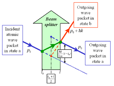
Figure 1: The continuous lines represent the central atomic trajectories (group velocities); the dashed lines refer to the equivalent instantaneous interaction (ttt scheme); and the dotted line is the extension of the initial atomic trajectory (infinitely thin modeling).

As for the central momentum, we obtain similarly the two following momenta:

$$\overrightarrow{p_{c}}\left(t,t_{0}\right)=mC\overrightarrow{r_{0}}+D\left(\overrightarrow{p_{0}}+\frac{\hbar\overrightarrow{k}}{2}\right)+m\overrightarrow{\phi}\pm\frac{\hbar\overrightarrow{k}}{2}$$

which differ from each other on $\hbar\overrightarrow{k}$, as expected.

On the contrary, $S_{op}$ may have a non-negligible effect on the external state of the incident wave packet (change of central position and momentum, respectively due to the addition of a non-trivial group velocity and to the change of momentum distribution). In this case, one can show that the initial wave packet is split into two main wave packets, which evolve along two different trajectories (i.e. with two distinct group velocities) which form the atomic Borrmann fan. For each of these wave packets, we can do the same calculation as before and obtain the trajectories in the initial frame [4].

5.3 Generalized ttt scheme

However, in both previous cases, it is noticeable that the expression (7) can be written as a product of three evolution operators:

$$\left|\Psi_{sol}\left(t\right)\right\rangle=U_{1}\left(t,t_{1}\right)\text{{\Large S}}_{{}_{1}}\left(\overrightarrow{r_{op}},\overrightarrow{p_{op}},t,t_{0},t_{1}\right)U_{1}\left(t_{1},t_{0}\right)\left|\Psi\left(t_{0}\right)\right\rangle$$

where $U_{1}\left(t_{1},t_{0}\right)$ and $U_{1}\left(t,t_{1}\right)$ describe the evolution due to $H_{0}+H_{ext}$ only, and where S${}_{{}_{1}}$ represents the evolution part depending on the splitting potential $V$. The aim of this arrangement is to clearly separate the effect of $H_{ext}$ and $V$, and to describe the interaction as an effective instantaneous interaction (generalization of the $ttt$ scheme introduced in [14]).

In addition to the link with the infinitely thin modeling of atomic beam splitters, we aim at providing a clear and practical beam splitter modeling, in the presence of the external fields described by $H_{ext}$, which can be used easily in atom interferometric phase shift calculations [56, 3, 4].

To clearly separate the splitting terms from the translation and phase terms in (8) and (9), we can transform the following expression:

$$e^{\pm\frac{i}{2}\Phi_{op}\left(t_{0},t_{1}\right)}\text{ }S_{uv}\left(\overrightarrow{r_{op}},\overrightarrow{p_{op}}\right)\text{ }e^{\mp\frac{i}{2}\Phi_{op}\left(t_{0},t_{1}\right)}$$

in [4]:

$$S_{uv}\left(\overrightarrow{r_{op}}\mp\widetilde{B}\left(t_{0},t_{1}\right)\frac{\hbar\overrightarrow{k}}{2m},\overrightarrow{p_{op}}\pm\widetilde{A}\left(t_{0},t_{1}\right)\frac{\hbar\overrightarrow{k}}{2}\right)$$

thanks to the following algebraic properties:

$$e^{A}.f\left(B\right).e^{-A} =f\left(e^{A}.B.e^{-A}\right)$$

$$e^{A}.B.e^{-A} =B+\left[A,B\right]+\frac{1}{2!}\left[A,\left[A,B\right]\right]+...$$

where $A$ and $B$ refer to operators or square matrices, and where $f$ is a function.

Finally, the diffusion matrix S₁ can be written as:

$$\text{{\Large S}}_{1}=\left(\begin{array}[c]{cc}\text{{\Large S}}_{1,bb}&\text{{\Large S}}_{1,ba}\\ \text{{\Large S}}_{1,ab}&\text{{\Large S}}_{1,aa}\end{array}\right)$$

where its elements are equal to ($a$ and $b$ are the lower and upper states respectively):

1. for the $a\longrightarrow a$ transition:

   $$\text{{\Large S}}_{1,aa}=e^{i\Phi_{aa}}e^{\frac{i}{\hbar}\overrightarrow{r_{op}}.\overrightarrow{p_{aa}}}e^{-\frac{i}{\hbar}\overrightarrow{p_{op}}.\overrightarrow{r_{aa}}}S_{aa}\left(\overrightarrow{r_{op}}-\widetilde{B}\left(t_{0},t_{1}\right)\frac{\hbar\overrightarrow{k}}{2m},\overrightarrow{p_{op}}+\widetilde{A}\left(t_{0},t_{1}\right)\frac{\hbar\overrightarrow{k}}{2}\right)$$

   with:

   $$\overrightarrow{p_{aa}} =-\frac{\widetilde{A}\left(t,t_{1}\right)-\widetilde{A}\left(t_{0},t_{1}\right)}{2}\hbar\overrightarrow{k}$$

   $$\overrightarrow{r_{aa}} =+\frac{\widetilde{B}\left(t,t_{1}\right)-\widetilde{B}\left(t_{0},t_{1}\right)}{2}\frac{\hbar\overrightarrow{k}}{m}$$

   $$\Phi_{aa} =+\frac{1}{2}\left[\left(\omega-\omega_{0}\right)\left(t-t_{0}\right)-\overrightarrow{k}.\left(\overrightarrow{\xi}\left(t,t_{1}\right)-\overrightarrow{\xi}\left(t_{0},t_{1}\right)\right)\right]$$

   $$+\frac{\hbar\overrightarrow{k}}{8m}\left[A\left(t,t_{1}\right)\widetilde{B}\left(t,t_{1}\right)+A\left(t_{0},t_{1}\right)\widetilde{B}\left(t_{0},t_{1}\right)-2A\left(t_{0},t_{1}\right)\widetilde{B}\left(t,t_{1}\right)\right]\overrightarrow{k}-\int_{t_{0}}^{t}\frac{\delta\left(t^{\prime},t_{1}\right)}{4}dt^{\prime}$$

2. for the $a\longrightarrow b$ transition:

   $$\text{{\Large S}}_{1,ba}=e^{i\Phi_{ba}}e^{\frac{i}{\hbar}\overrightarrow{r_{op}}.\overrightarrow{p_{ba}}}e^{-\frac{i}{\hbar}\overrightarrow{p_{op}}.\overrightarrow{r_{ba}}}S_{ba}\left(\overrightarrow{r_{op}}-\widetilde{B}\left(t_{0},t_{1}\right)\frac{\hbar\overrightarrow{k}}{2m},\overrightarrow{p_{op}}+\widetilde{A}\left(t_{0},t_{1}\right)\frac{\hbar\overrightarrow{k}}{2}\right)$$

   with:

   $$\overrightarrow{p_{ba}} =+\frac{\widetilde{A}\left(t,t_{1}\right)+\widetilde{A}\left(t_{0},t_{1}\right)}{2}\hbar\overrightarrow{k}$$

   $$\overrightarrow{r_{ba}} =-\frac{\widetilde{B}\left(t,t_{1}\right)+\widetilde{B}\left(t_{0},t_{1}\right)}{2}\frac{\hbar\overrightarrow{k}}{m}$$

   $$\Phi_{ba} =-\left[\omega\frac{t+t_{0}}{2}-\omega_{0}\left(\frac{t+t_{0}}{2}-t_{1}\right)+\phi-\overrightarrow{k}.\frac{\overrightarrow{\xi}\left(t,t_{1}\right)+\overrightarrow{\xi}\left(t_{0},t_{1}\right)}{2}\right]$$

   $$+\frac{\hbar\overrightarrow{k}}{8m}\left[A\left(t,t_{1}\right)\widetilde{B}\left(t,t_{1}\right)+A\left(t_{0},t_{1}\right)\widetilde{B}\left(t_{0},t_{1}\right)+2A\left(t_{0},t_{1}\right)\widetilde{B}\left(t,t_{1}\right)\right]\overrightarrow{k}-\int_{t_{0}}^{t}\frac{\delta\left(t^{\prime},t_{1}\right)}{4}dt^{\prime}$$

3. for the $b\longrightarrow a$ transition:

   $$\text{{\Large S}}_{1,ab}=e^{i\Phi_{ab}}e^{\frac{i}{\hbar}\overrightarrow{r_{op}}.\overrightarrow{p_{ab}}}e^{-\frac{i}{\hbar}\overrightarrow{p_{op}}.\overrightarrow{r_{ab}}}S_{ab}\left(\overrightarrow{r_{op}}+\widetilde{B}\left(t_{0},t_{1}\right)\frac{\hbar\overrightarrow{k}}{2m},\overrightarrow{p_{op}}-\widetilde{A}\left(t_{0},t_{1}\right)\frac{\hbar\overrightarrow{k}}{2}\right)$$

   with:

   $$\overrightarrow{p_{ab}} =-\frac{\widetilde{A}\left(t,t_{1}\right)+\widetilde{A}\left(t_{0},t_{1}\right)}{2}\hbar\overrightarrow{k}$$

   $$\overrightarrow{r_{ab}} =+\frac{\widetilde{B}\left(t,t_{1}\right)+\widetilde{B}\left(t_{0},t_{1}\right)}{2}\frac{\hbar\overrightarrow{k}}{m}$$

   $$\Phi_{ab} =+\left[\omega\frac{t+t_{0}}{2}-\omega_{0}\left(\frac{t+t_{0}}{2}-t_{1}\right)+\phi-\overrightarrow{k}.\frac{\overrightarrow{\xi}\left(t,t_{1}\right)+\overrightarrow{\xi}\left(t_{0},t_{1}\right)}{2}\right]$$

   $$+\frac{\hbar\overrightarrow{k}}{8m}\left[A\left(t,t_{1}\right)\widetilde{B}\left(t,t_{1}\right)+A\left(t_{0},t_{1}\right)\widetilde{B}\left(t_{0},t_{1}\right)+2A\left(t_{0},t_{1}\right)\widetilde{B}\left(t,t_{1}\right)\right]\overrightarrow{k}-\int_{t_{0}}^{t}\frac{\delta\left(t^{\prime},t_{1}\right)}{4}dt^{\prime}$$

4. for the $b\longrightarrow b$ transition:

   $$\text{{\Large S}}_{1,bb}=e^{i\Phi_{bb}}e^{\frac{i}{\hbar}\overrightarrow{r_{op}}.\overrightarrow{p_{bb}}}e^{-\frac{i}{\hbar}\overrightarrow{p_{op}}.\overrightarrow{r_{bb}}}S_{bb}\left(\overrightarrow{r_{op}}+\widetilde{B}\left(t_{0},t_{1}\right)\frac{\hbar\overrightarrow{k}}{2m},\overrightarrow{p_{op}}-\widetilde{A}\left(t_{0},t_{1}\right)\frac{\hbar\overrightarrow{k}}{2}\right)$$

   où:

   $$\overrightarrow{p_{bb}} =+\frac{\widetilde{A}\left(t,t_{1}\right)-\widetilde{A}\left(t_{0},t_{1}\right)}{2}\hbar\overrightarrow{k}$$

   $$\overrightarrow{r_{bb}} =-\frac{\widetilde{B}\left(t,t_{1}\right)-\widetilde{B}\left(t_{0},t_{1}\right)}{2}\frac{\hbar\overrightarrow{k}}{m}$$

   $$\Phi_{bb} =-\frac{1}{2}\left[\left(\omega-\omega_{0}\right)\left(t-t_{0}\right)-\overrightarrow{k}.\left(\overrightarrow{\xi}\left(t,t_{1}\right)-\overrightarrow{\xi}\left(t_{0},t_{1}\right)\right)\right]$$

   $$+\frac{\hbar\overrightarrow{k}}{8m}\left[A\left(t,t_{1}\right)\widetilde{B}\left(t,t_{1}\right)+A\left(t_{0},t_{1}\right)\widetilde{B}\left(t_{0},t_{1}\right)-2A\left(t_{0},t_{1}\right)\widetilde{B}\left(t,t_{1}\right)\right]\overrightarrow{k}-\int_{t_{0}}^{t}\frac{\delta\left(t^{\prime},t_{1}\right)}{4}dt^{\prime}$$

The interpretation of these terms is simple and constitutes the core of the generalized $ttt$ scheme:

1. from $t_{0}$ to $t_{1}$, the initial ket $\left|\Psi\left(t_{0}\right)\right\rangle$ evolves with $H_{0}+H_{ext}$ only (as if there was no splitting potential);

2. at $t_{1}$, this evolved ket is subject to an effective instantaneous interaction which modifies its structure (structuring into several wave packets, see part 6 and the illustration of the ttt scheme on figure 2), its central position and momentum, and its phase;

3. from $t_{1}$ to $t$, the obtained wave packets evolve with $H_{0}+H_{ext}$ only, as before $t_{1}$.

Eventually, we can show that the $t_{1}$ value which simplifies the most the previous expressions is the central time of interaction:

$$t_{1}=t_{1/2}=\frac{t+t_{0}}{2}$$

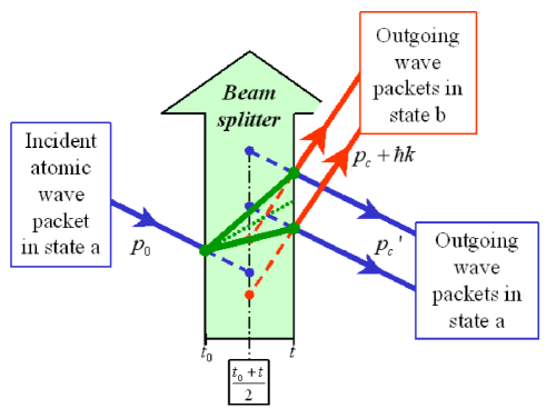
Figure 2: Atomic beam splitting in the free case and for an inelasticity parameter different from zero. The dashed lines refer to the ttt scheme, whereas the dotted line represents the common atomic trajectory of the Borrmann effect.

Let us see now what are the features of the wave packets which appear inside the beam splitters. Before studying this wave packet structuring in the general case (i.e. in the presence of trapping and gravito-inertial potentials), we will focus on the simple “free” case (i.e. without any such other external potential).

6 Structure of the solutions in the free case

The study of the free case is important for at least two reasons. First, as we have seen in part 3, the effect of the quadratic terms of $H_{ext}$ (rotations, gradients, trap…) can often be neglected during the resolution of equation (5), and any uniform acceleration can be easily removed by modulating the laser frequency. In this case, the equation (5) is equivalent to the one stemming from the free case. Second, and as far as we know, to date, there has been no global study of matter wave beam splitters even in the simplest free case. Indeed, each of the previously quoted works aims at studying only a few aspects of the atomic beam splitting: mechanical effect, internal and external splitting, group velocities… Actually, the question consisting in finding what exactly goes out of an atomic beam splitter is still relevant, even for a simple laser potential (temporal square amplitude) and an incident Gaussian matter wave packet.

It is therefore necessary to specify what is the exact structuring of this incident wave packet, namely the number of created wave packets (two main ones for each transition amplitude), their amplitude (Rabi oscillations, velocity selection, anomalous dispersion…), their group velocity (Borrmann fan), their central momentum and their phase, and eventually how these quantities evolve in time.

6.1 Group velocities and adiabatic states

The laser-atom interaction induces particular states, the adiabatic or dressed states, which are nothing but the eigenstates of the interaction. If $\overline{F}\left(t,t_{1}\right)$ is a unit amplitude square pulse between $t_{0}$ and $t$, these adiabatic states are simply the eigenvectors of the matrix $iM\left(1/2,t\right)$. Therefore, the two corresponding eigenenergies are:

$$\mp\varepsilon\left(\overrightarrow{p}\right)=\mp\hbar\sqrt{\Omega_{0}^{2}+\left[\Delta_{l}\left(\overrightarrow{p}\right)/2\right]^{2}}$$

with $\Delta_{l}\left(\overrightarrow{p}\right)=\omega-\omega_{0}-\overrightarrow{k}.\overrightarrow{p}/m$, and the corresponding group velocities are simply obtained by deriving these dispersion relations with respect to the momentum:

$$\pm\overrightarrow{v_{g}}\left(\overrightarrow{p}\right)=\mp\frac{y\left(\overrightarrow{p}\right)}{\sqrt{1+y\left(\overrightarrow{p}\right)^{2}}}\frac{\hbar\overrightarrow{k}}{2m}$$

where $y\left(\overrightarrow{p}\right)$ is the well known “off Braggness parameter” introduced in neutron optics [55, 16] and defined here as:

$$y\left(\overrightarrow{p}\right)=\left(\omega-\omega_{0}-\overrightarrow{k}.\overrightarrow{p}/m\right)/2\Omega_{0}$$

As we can see on (8) and (9), the matrices $S_{uv,op}$ act on a wave packet which is shifted by a global momentum of $+\hbar\overrightarrow{k}/2$ or $-\hbar\overrightarrow{k}/2$, depending on the initial internal state of atoms. For the example previously described (atoms initially in the lower internal state), we obtain the following parameter:

$$y\left(\overrightarrow{p}+\hbar\overrightarrow{k}/2\right)=y_{+}\left(\overrightarrow{p}\right)=\left(\omega-\omega_{0}-\overrightarrow{k}.\overrightarrow{p}/m-\delta\right)/2\Omega_{0}$$ (10)

which can be called “inelasticity parameter” as it refers to the way the resonance condition is fulfilled [4]. In the initial representation, these group velocities become:

$$\frac{\overrightarrow{p}}{m}+\frac{\hbar\overrightarrow{k}}{2m}\left(1\pm\frac{y_{+}\left(\overrightarrow{p}\right)}{\sqrt{1+y_{+}\left(\overrightarrow{p}\right)^{2}}}\right)$$

The examination of these velocities leads to several important conclusions.

First, the difference between momentum and group velocity in the presence of an electromagnetic field is naturally confirmed. For a weak inelasticity parameter $\left|y_{+}\left(\overrightarrow{p}\right)\right|\ll 1$, we obtain only one group velocity for both the adiabatic states (atomic Borrmann effect, see part 5.2):

$$\frac{\overrightarrow{p}}{m}+\frac{\hbar\overrightarrow{k}}{2m}$$

whereas for $\left|y_{+}\left(\overrightarrow{p}\right)\right|\gg 1$, we obtain the two extreme velocities (defining the Borrmann fan):

$$\frac{\overrightarrow{p}}{m}\text{ \ and \ }\frac{\overrightarrow{p}}{m}+\frac{\hbar\overrightarrow{k}}{m}$$

But in this case, the beam splitter is inefficient as we will see thereafter.

However, we can show [4] that these group velocities are closely linked to the average momenta of the considered two level system, and that they are more precisely equal to the most probable momenta of adiabatic states (divided by $m$).

For $y\neq 0$, two distinct atomic wave packets are created in the beam splitter, and their physical separation may be observable in certain conditions (more than few $\mu m$ after $10^{-4}$ $s$ for an initial atomic coherent state of $1$ $\mu m$ width).

Finally, it is noteworthy that these group velocities depend on $\overrightarrow{p}$. Therefore, the (optical) medium where atoms evolve is dispersive and this effect leads to the phenomenon of anomalous dispersion (see part 6.4).

6.2 Rabi oscillations

Let us consider the free solution of equation (5). If the internal state of initial atoms is the lower state, we obtain in the initial picture the following lower state:

$$T_{aa}\left(\overrightarrow{p_{op}},t\right)\left|a\left(t_{0}\right)\right\rangle$$

with:

$$T_{aa}\left(\overrightarrow{p},t\right)=\exp\left[-i\left(\frac{E_{a}}{\hbar}+\left(\overrightarrow{p}+\frac{\hbar\overrightarrow{k}}{2}\right)^{2}/2m\hbar+\frac{\delta}{4}-\frac{\omega-\omega_{0}}{2}\right)\left(t-t_{0}\right)\right]S_{aa}\left(\overrightarrow{p}+\frac{\hbar\overrightarrow{k}}{2}\right)$$

and the following upper state:

$$e^{-i\left(\omega t_{0}-\overrightarrow{k}.\overrightarrow{r_{op}}+\phi\right)}T_{ba}\left(\overrightarrow{p_{op}},t\right)\left|a\left(t_{0}\right)\right\rangle$$

with:

$$T_{ba}\left(\overrightarrow{p},t\right)=\exp\left[-i\left(\frac{E_{b}}{\hbar}+\left(\overrightarrow{p}+\frac{\hbar\overrightarrow{k}}{2}\right)^{2}/2m\hbar+\frac{\delta}{4}+\frac{\omega-\omega_{0}}{2}\right)\left(t-t_{0}\right)\right]S_{ba}\left(\overrightarrow{p}+\frac{\hbar\overrightarrow{k}}{2}\right)$$

$S_{aa}$ and $S_{ba}$ having the following usual expressions:

$$S_{aa}\left(\overrightarrow{p},t-t_{0}\right)=\cos\left[\varepsilon\left(\overrightarrow{p}\right).\left(t-t_{0}\right)\right]-i\frac{y\left(\overrightarrow{p}\right)}{\sqrt{1+y\left(\overrightarrow{p}\right)^{2}}}\sin\left[\varepsilon\left(\overrightarrow{p}\right).\left(t-t_{0}\right)\right]$$

$$S_{ba}\left(\overrightarrow{p},t-t_{0}\right)=i\frac{1}{\sqrt{1+y\left(\overrightarrow{p}\right)^{2}}}\sin\left[\varepsilon\left(\overrightarrow{p}\right).\left(t-t_{0}\right)\right]$$

The temporal evolution of the initial state is therefore sinusoidal with an amplitude equal to $1/\left(1+y_{+}\left(\overrightarrow{p}\right)^{2}\right)$ and a frequency equal to $\Omega_{0}\sqrt{1+y_{+}\left(\overrightarrow{p}\right)^{2}}/2\pi$. Tuning the interaction parameters, we can realize true atomic mirrors or “$\pi$ pulses” (transfer of all the atoms from one state to another) and semi-reflecting plates or “$\pi/2$ pulses” (50-50 splitting), whose efficiency depends in a crucial way of the value of $y_{+}\left(\overrightarrow{p}\right)$ which is actually taken by the central momentum of the incident wave packet.

6.3 Velocity selection

This effect comes from the fact that the two pre-factors $1/\sqrt{1+y_{+}\left(\overrightarrow{p}\right)^{2}}$ and $y_{+}\left(\overrightarrow{p}\right)/\sqrt{1+y_{+}\left(\overrightarrow{p}\right)^{2}}$, in the expression of $S_{aa}$ and $S_{ba}$, depend on the momentum $\overrightarrow{p}$, and more particularly on its part which is collinear to the laser wave vector $\overrightarrow{k}$ (transverse momentum). Therefore, the terms $S_{uv}$ act as momentum filters on the incident atomic momentum distribution.

For example, in the case of the $a\longrightarrow b$ transition, one obtains the well known sinus cardinal filter. It is characterized by a central lobe with an amplitude of $\sin\left[\Omega_{0}\tau\right]$ and a total width of $4\Omega_{0}\left(\sqrt{\left(\pi/\Omega_{0}\tau\right)^{2}-1}\right)/k$ (for a fixed interaction duration of $\tau=t-t_{0}$). This width may be less than the transverse width of the incident atomic momentum distribution. The resulting (transverse) velocity selection is very useful in atom interferometry (to increase the fringes contrast) and constitutes the basis of Raman cooling [57].

Furthermore, this central lobe is centered on the transverse momentum $p_{l}$:

$$p_{l}=m\left(\omega-\omega_{0}-\delta\right)/k$$

which can be quite different from the initial transverse central momentum $\overrightarrow{p_{0}}.\overrightarrow{k}/k$. If so, the central momentum $\overrightarrow{p_{c}}$ of the filtered distribution is distinct from $\overrightarrow{p_{0}}$ and is bounded by $\overrightarrow{p_{0}}$ and $\overrightarrow{p_{l}}$. Consequently, the central momentum of the outgoing wave packets (in excited state) is not $\overrightarrow{p_{0}}+\hbar\overrightarrow{k}$, as one would think in view of the mechanical recoil effect of light, but $\overrightarrow{p_{c}}+\hbar\overrightarrow{k}$ (see Figure 3).

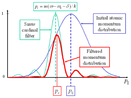
Figure 3: Transverse momentum distribution, before and after filtering by a $\pi$ beam splitter, of a Gaussian atomic wave packet.

Apart from the central lobe, the $sinc$ filter has nodes and sidelobes with an amplitude that rapidly decreases (this particular structure is linked to the pulse shape, and can be softened or removed by the use of apodization functions [Blackman for example] to tailor laser pulses). If the incident atomic distribution is sufficiently broad to encompass one or several sidelobes, the filtered matter wave packet will then be structured into several wave packets whith central momenta quite different from $\overrightarrow{p_{0}}$, $\overrightarrow{p_{l}}$ or $\overrightarrow{p_{c}}$.

With respect to the other transition amplitude ($a\longrightarrow a$, i.e. without change of internal state), we obtain the complement filter and the structuring can be studied in the same way [4].

6.4 Anomalous dispersion

This effect refers to the modification of spreading of atomic wave packets inside a beam splitter. It is more convenient to examine it for an incident atomic wave packet which has a thin momentum distribution, although it can be studied and modeled for any momentum distribution (see [4]).

As we consider the wave packets which evolve inside the beam splitter, we have to go into the adiabatic states. In the adiabatic picture, these wave packets have the two energies (written here for the $a\longrightarrow b$ transition):

$$\pm\hbar\Omega_{0}\sqrt{1+y_{+}\left(\overrightarrow{p}\right)^{2}}$$

where the term $\sqrt{1+y_{+}\left(\overrightarrow{p}\right)^{2}}$ can be Taylor expanded with respect to $\overrightarrow{k}.\left(\overrightarrow{p}-\overrightarrow{p_{0}}\right)/2m\Omega_{0}$ as:

$$\sqrt{1+y_{+}\left(\overrightarrow{p}\right)^{2}}=\sqrt{1+y_{0+}^{2}}-\frac{y_{0+}}{\sqrt{1+y_{0+}^{2}}}\frac{\overrightarrow{k}.\left(\overrightarrow{p}-\overrightarrow{p_{0}}\right)}{2m\Omega_{0}}+\frac{1}{\left(1+y_{0+}^{2}\right)^{3/2}}\frac{\left(\overrightarrow{p}-\overrightarrow{p_{0}}\right).\overset{\Rightarrow}{\delta}.\left(\overrightarrow{p}-\overrightarrow{p_{0}}\right)}{4m\hbar\Omega_{0}^{2}}+...$$

where $y_{0+}$ is defined as:

$$y_{0+}=y_{+}\left(\overrightarrow{p_{0}}\right)$$

and where $\overset{\Rightarrow}{\delta}$ is the complement matrix of the recoil term $\delta$:

$$\overset{\Rightarrow}{\delta}=\frac{\hbar\overrightarrow{k}.\widetilde{\overrightarrow{k}}}{2m}=\frac{\hbar}{2m}\left(\begin{array}[c]{ccc}k_{x}^{2}&k_{x}k_{y}&k_{x}k_{z}\\ k_{x}k_{y}&k_{y}^{2}&k_{y}k_{z}\\ k_{x}k_{z}&k_{y}k_{z}&k_{z}^{2}\end{array}\right)$$

In the initial picture, the first order term of this expansion gives the group velocities obtained in part 6.1. As for the second order term, it corresponds to an additional dispersion and it indicates that one wave packet spreads more than the natural spreading, and that the other one spreads less. In certain conditions, this spreading can even be stopped or changed into a contraction [4, 11].

In the case of a non-thin incident atomic wave packet, the main results of this study are still valid provided $y_{0+}$ is changed into $y_{c+}=y_{+}\left(\overrightarrow{p_{c}}\right)$. One can then model the outgoing atomic wave packets. A simple but powerful way to do this is the Gaussian modeling which consists in writing these wave packets as Gaussians. This “strong field ttt modeling”, and more generally the use of Gaussian wave packets, is found to be particularly relevant in atom interferometry (see [4]).

7 Structure of the solutions in the general case

We have already seen in part 4 how to deal with the double non-commutation problem which appears in $\Delta_{op1}$ and in the resolution of (5). In particular, we have seen that one can often neglect, in the expression of $\Delta_{op1}$, the terms depending on the quadratic terms of $H_{ext}$, namely $\alpha$, $\beta-1$ and $\gamma$. In certain configurations (when $\overrightarrow{k}$ is orthogonal to $\overrightarrow{g}$ or when $\omega$ is modulated to compensate the gravity induced Doppler shift), the generalized detuning is even equal to the free one and it boils down to the free case in (and only in) the resolution of (5).

In this case, we obtain the same previous adiabatic energies and consequently the same adiabatic group velocities, Rabi oscillations, velocity selection and anomalous dispersion effect as stated before. In the initial picture (i.e. in the lab frame), the elements of the previous S${}_{{}_{1}}$ matrix are therefore expressed as ($u,v=a,b$):

$$\text{{\Large S}}_{1,uv}=\exp\left[i\Phi_{uv}\right].\exp\left[\frac{i}{\hbar}\overrightarrow{r_{op}}.\overrightarrow{p_{uv}}\right].\exp\left[-\frac{i}{\hbar}\overrightarrow{p_{op}}.\overrightarrow{r_{uv}}\right].S_{uv}\left(\overrightarrow{p_{op}}\mp\frac{\hbar\overrightarrow{k}}{2}\right)$$

where the elements $S_{uv}$ are equal to the ones obtained in the free case (see the previous part).

Finally, the only differences from the free case lie in the expression of:

1. the effective incident wave packet at time $t_{1}$ (which is equal to the initial wave packet evolved from $t_{0}$ to $t_{1}$ thanks to $H_{0}+H_{ext}$). In particular, its central position and momentum are no more $\overrightarrow{r_{0}}+\overrightarrow{p_{0}}\left(t_{1}-t_{0}\right)/m$ and $\overrightarrow{p_{0}}$ but $\overrightarrow{R}\left(t_{1},t_{0},\overrightarrow{r_{0}},\overrightarrow{p_{0}}\right)$ and $\overrightarrow{P}\left(t_{1},t_{0},\overrightarrow{r_{0}},\overrightarrow{p_{0}}\right)$ (expressed with the $ABCD$ matrices, see part 3)

2. the terms $\overrightarrow{r_{uv}}$, $\overrightarrow{p_{uv}}$ and $\Phi_{uv}$ which are detailed in part 5.3

3. $U_{1}\left(t,t_{1}\right)$ which accounts for the evolution from $t_{1}$ to $t$ due to $H_{0}+H_{ext}$.

Then, we can do the same Gaussian modeling as in the free case previously studied (see [4]).

In some cases however, we can not neglect the effect of (unavoidable) gravitational, inertial and trapping potentials for the resolution of (5), and it is important to examine what are the changes, due to $H_{ext}$, of the properties listed before (group velocities, Rabi oscillations, velocity selection and anomalous dispersion). Moreover, we have already underlined that the key parameter is the inelasticity parameter $y$ which is proportional to the generalized detuning $\Delta$. This $y$ parameter generally depends on the two canonical operators $\overrightarrow{r_{op}}$ and $\overrightarrow{p_{op}}$, but in the case of linear potentials (uniform acceleration for example) it depends on one operator ($\overrightarrow{p_{op}}$) only.

Before dealing with the general case, let us consider the effect of a uniform (but time-dependent) acceleration $\overrightarrow{g}\left(t\right)$. From the equation (5), which becomes scalar in momentum representation, one can extract the adiabatic energies and then the adiabatic group velocities (written here for $t_{1}=t_{0}$):

$$\pm\overrightarrow{v_{g0}}\left(t,t_{0}\right)=\mp\frac{y_{0}}{\sqrt{1+y_{0}^{2}}}\frac{\hbar\overrightarrow{k}}{2m}$$

with ($\overline{F}$ is taken constant and equal to $1$ for simplicity):

$$y_{0}=y\left(\overrightarrow{p_{0}}\right)=y_{0free}-\overrightarrow{k}.\int_{t_{0}}^{t}\overrightarrow{g}\left(t^{\prime}\right)dt^{\prime}/2\Omega_{0}$$

where $y_{0free}$ is the inelasticity parameter obtained without $\overrightarrow{g}$ (free case, see (10)).

In the initial picture, this result becomes eventually:

$$\frac{\overrightarrow{p_{0}}}{m}+\frac{\hbar\overrightarrow{k}}{2m}+\int_{t_{0}}^{t}\overrightarrow{g}\left(t^{\prime}\right)dt^{\prime}\pm\overrightarrow{v_{g0}}$$

where two sources of atomic trajectories bending can be identified: the common gravitational bending coming from the third term $\int_{t_{0}}^{t}\overrightarrow{g}\left(t^{\prime}\right)dt^{\prime}$, and an “anomalous gravity induced Doppler bending” coming from the time-dependent adiabatic group velocities. As for the free case, this anomalous bending can be described either in terms of effective mass tensors [12, 11] or in terms of position (and time) dependent effective refractive index inside the beam splitter [11, 58].

Let us remark that the acceleration induced Doppler term $-\overrightarrow{k}.\overrightarrow{g}$ may produce a non-trivial bending of central atomic trajectories. Indeed, if $y_{0free}$ and the scalar $\overrightarrow{k}.\overrightarrow{g}$ are non zero, and if $y_{0free}$ has the same sign as $\overrightarrow{k}.\overrightarrow{g}$, then the trajectories bending due to the $\overrightarrow{k}.\overrightarrow{g}$ term makes these trajectories get closer (as usually considered in literature). On the contrary, if $y_{0free}$ has the opposite sign of $\overrightarrow{k}.\overrightarrow{g}$, then these two main trajectories repel each other (see Figure 4). In both cases, if the vectors $\overrightarrow{k}$ and $\overrightarrow{g}$ point at the same direction ($\overrightarrow{k}.\overrightarrow{g}>0$), downward for example, then one of the two main atomic wave packets will always be accelerated upward, even if all “forces” (acceleration and laser pulse) seem to push the atoms downward.

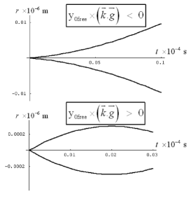
Figure 4: Central atomic trajectories inside a (temporal) beam splitter in the presence of Earth gravity: adiabatic picture. Numerical application: $k=10^{7}m^{-1}$, $g=10m.s^{-2}$, $\Omega_{0}=3.10^{3}s^{-1}$, $y_{0free}=\pm 0.1$, $t_{0}=0s$. The central atomic trajectories either attract or repel each other.

Furthermore, this particular behavior is not limited to the adiabatic picture and can be observed fully in the laboratory frame (i.e. in the initial picture). Indeed, if $\delta>2\Omega_{0}\left(1+y_{0free}^{2}\right)^{3/2}$ (which corresponds, for $y_{0free}=0$, to the “Bragg regime”, as it is defined in [59] in contrast with the “channeling regime” for which $\delta<2\Omega_{0}$), this anomalous upward acceleration exceeds the downward acceleration of gravity (for $t-t_{0}$ much less than $1/\Omega_{0}$). As a result, some atoms are accelerated upward in the lab frame, even if the action of $\overrightarrow{g}$ and laser beams is directed downward (see Figure 5). Of course, this anomalous “anti-gravitational” bending can be explained simply by considering the conservation of momentum and energy during the interaction process.

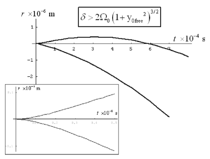
Figure 5: Central atomic trajectories inside a (temporal) beam splitter in the presence of Earth gravity: initial picture (lab frame). Numerical application: $k=10^{7}m^{-1}$, $g=10m.s^{-2}$, $\Omega_{0}=3.10^{3}s^{-1}$, $y_{0free}=-0.1$, $t_{0}=0s$. For short times, the anomalous upward acceleration exceeds the downward acceleration of gravity.

In the general case of an at-most-quadratic $H_{ext}$ (with quadratic terms like rotations, gradients of acceleration, trapping potentials, etc), the generalized detuning $\Delta_{op1}$ depends on the two non-commuting canonical operators, and it can not be made scalar in any representation. As we saw previously, one of the most relevant strategies is to approximate, in the resolution of equation (5), the effect of one of these two operators by considering its action on a typical atomic wave packet which evolves inside the beam splitter. In the free case, the Gaussian approximation of these typical wave packets, called here “wp” for convenience, leads to (in the adiabatic picture):

$$\overrightarrow{r_{op}}\left(wp\right)\simeq\left(\overrightarrow{r_{0}}\pm\int_{t_{0}}^{t}\overrightarrow{v_{g0}}\left(t^{\prime},t_{0}\right)dt^{\prime}+\left(U_{0}\mp U_{AD}\right).\left(\overrightarrow{p}-\overrightarrow{p_{0}}\right)\right).wp$$ (11)

where $U_{0}$ is linked to the complex momentum width of the initial atomic wave packet, and where $U_{AD}$ accounts for the anomalous dispersion phenomenon.

In fact, we can make $U_{AD}$ arbitrarily small (for a sufficiently small interaction duration) and incorporate the time-independent matrix $U_{0}$ into the expression of $y$ (see (6) and (10)), and consider only the two first terms of (11). Finally, the quantity $\overrightarrow{x}\left(t\right)=\int_{t_{0}}^{t}\overrightarrow{v_{g0}}\left(t^{\prime},t_{0}\right)dt^{\prime}$ meets the following first order differential equation (which can be solved numerically):

$$\frac{d}{dt}\overrightarrow{x}=-\frac{\overline{y_{0}}-\overrightarrow{k}.\overset{\cdot}{A}\left(t,t_{0}\right).\overrightarrow{x}/2\Omega_{0}\overline{F}\left(t\right)}{\sqrt{1+\left(\overline{y_{0}}-\overrightarrow{k}.\overset{\cdot}{A}\left(t,t_{0}\right).\overrightarrow{x}/2\Omega_{0}\overline{F}\left(t\right)\right)^{2}}}\overset{\cdot}{\widetilde{B\left(t,t_{0}\right)}}\frac{\hbar\overrightarrow{k}}{2m}$$

with:

$$\overline{y_{0}}=\left(\omega-\omega_{0}-\delta-\overrightarrow{k}.\overset{\cdot}{A}\left(t,t_{0}\right).\overrightarrow{r_{0}}-\overrightarrow{k}.\overset{\cdot}{B}\left(t,t_{0}\right).\overrightarrow{p_{0}}/m-\overrightarrow{k}.\overset{\cdot}{\overrightarrow{\xi}}\left(t,t_{0}\right)\right)/2\Omega_{0}\overline{F}\left(t\right)$$

A simpler approximation (WKB approximation) amounts to neglecting also $\int_{t_{0}}^{t}\overrightarrow{v_{g0}}\left(t^{\prime},t_{0}\right)dt^{\prime}$ in the expression (11). In this case, we obtain readily:

$$\pm\overrightarrow{v_{g0}}\left(t,t_{0}\right)=\mp\frac{\overline{y_{0}}}{\sqrt{1+\overline{y_{0}}^{2}}}\overset{\cdot}{\widetilde{B\left(t,t_{0}\right)}}\frac{\hbar\overrightarrow{k}}{2m}$$

which gives a good approximation of the group velocities inside a matter wave beam splitter when this latter is subject to the various external potentials described by $H_{ext}$.

For example, for a non-uniform (but time-independent) acceleration $\left(\overrightarrow{g},\gamma\right)$ (or in the case of a trapping potential, for which the sign of $\gamma$ has to be reversed), one obtains:

$$\overline{y_{0}} =\left(\omega-\omega_{0}-\delta-\overrightarrow{k}.\cosh\left(\gamma^{1/2}\left(t-t_{0}\right)\right).\overrightarrow{p_{0}}/m\right.$$

$$\left.-\overrightarrow{k}.\gamma^{1/2}\sinh\left(\gamma^{1/2}\left(t-t_{0}\right)\right).\overrightarrow{r_{0}}-\overrightarrow{k}.\gamma^{-1/2}\sinh\left(\gamma^{1/2}\left(t-t_{0}\right)\right).\overrightarrow{g}\right)/2\Omega_{0}\overline{F}\left(t\right)$$

Similarly, in the case of a (time-independent) rotation $\overrightarrow{\Omega}$, one obtains:

$$\overline{y_{0}}=\left(\omega-\omega_{0}-\delta-\overrightarrow{k}.\mathcal{R}\left(t,t_{0}\right).\left[\overrightarrow{p_{0}}/m-\overrightarrow{\Omega}\times\left(\overrightarrow{r_{0}}+\overrightarrow{p_{0}}\left(t-t_{0}\right)/m\right)\right]\right)/2\Omega_{0}\overline{F}\left(t\right)$$

where the rotation matrix $\mathcal{R}\left(t,t_{0}\right)$ can be seen as acting either on the atomic wave packet or on the wave vector $\overrightarrow{k}$.

8 Conclusion

In conclusion, we have shown in this paper how to solve the problem of matter wave splitting in the presence of various gravitational, inertial and trapping potentials. In particular, we have seen how the resonance condition between the splitting potential and the effective two-level atoms has to be changed. Then, we have shown how to express this triple interaction “matter - splitting potential - other external potentials” as an equivalent instantaneous interaction (generalized $ttt$ scheme).

Finally, we have investigated in detail what is the dispersive structuring of an incident atomic wave packet inside such beam splitters, both in the free case (for which $H_{ext}$ is reduced to $\overrightarrow{p}^{2}/2m$) and in the general case of $H_{ext}$. Several significant features of the solutions have been studied: group velocities, generalized Rabi oscillations, velocity selection, anomalous dispersion effects… In the light of this study, the generalized $ttt$ scheme leads to a very practical and efficient (Gaussian) modeling of atomic beam splitters which is particularly relevant for atom interferometric signal calculations [3, 4].

It is worth pointing out that these results stem from a strong field theory for both the splitting potential and the other external potentials described by $H_{ext}$.

However, several points still have to be cleared up: for instance, the problem of the effective mass change which occurs when the atomic internal state is changed, and which leads to non-trivial (small) relativistic corrections. Furthermore, it is necessary to extend our formalism to additional external potentials which are more than quadratic (in position and momentum) if we want to investigate the effect of van-der-Waals, Casimir or Yukawa-type potentials on the matter wave splitting. More generally speaking, it would be interesting to go beyond the various approximations listed in part 2, and in particular beyond the two-beam approximation.

References

- [1] T.L. Gustavson, A. Landragin and M.A. Kasevich., Class. Quantum Grav. 17, 2385 (2000); A. Peters, K.Y. Chung and S. Chu, Metrologia 38, 25 (2001); J.M. McGuirk, G.T. Foster, J.B. Fixler, M.J. Snadden, and M.A. Kasevich, Phys. Rev. A 65, 033608 (2002); G. Wilpers, T. Binnewies, C. Degenhardt, U. Sterr, J. Helmcke, and F. Riehle, Phys. Rev. Lett. 89, 230801 (2002).
- [2] Ch. J. Bordé, N. Courtier, F. du Burck, A.N. Goncharov and M. Gorlicki, Phys. Lett. A 188, 187 (1994).
- [3] Ch. Antoine and Ch.J. Bordé, J. Opt. B: Quantum Semiclass. Opt. 5, S199 (2003).
- [4] Ch. Antoine, Contribution à la théorie des interféromètres atomiques, Ph.D. thesis (in French), Université Pierre et Marie Curie, Paris (2004).
- [5] F.T. Hioe and C.E. Caroll, Phys. Rev. A 32, 1541 (1985).
- [6] K.-A. Suominen and B.M. Garraway, Phys. Rev. A 45, 374 (1992).
- [7] J. Ishikawa, F. Riehle, J. Helmcke and Ch.J. Bordé, Phys. Rev. A 49, 4794 (1994).
- [8] L. Carmel and A. Mann, Phys. Rev. A 61, 052113 (2000).
- [9] A.M. Ishkhanyan, Opt. Comm. 176, 155 (2000).
- [10] M.K. Oberthaler, R. Abfalterer, S. Bernet, J. Schmiedmayer, and A. Zeilinger , Phys. Rev. Lett. 77, 4980 (1996); Ch.J. Bordé and C. Lämmerzahl, Ann. Phys. (Leipzig) 8, 83 (1999).
- [11] B. Eiermann, P. Treutlein, Th. Anker, M. Albiez, M. Taglieber, K.-P. Marzlin and M. K. Oberthaler, Phys. Rev. Lett. 91, 060402 (2003); B. Eiermann, Th. Anker, M. Albiez, M. Taglieber, P. Treutlein, K.-P. Marzlin and M. K. Oberthaler, Phys. Rev. Lett. 92, 230401 (2004).
- [12] C. Lämmerzahl and Ch.J. Bordé, Gen. Rel. Grav. 31, 635 (1999).
- [13] C. Lämmerzahl and Ch.J. Bordé, Phys. Lett. A 203, 59 (1995); K.-P. Marzlin and J. Audretsch, Phys. Rev. A 53, 1004 (1996).
- [14] Ch.J. Bordé, Gen. Rel. Grav. 36, 475 (2004).
- [15] M.A . Horne, Physica A 137, 260 (1986).
- [16] H. Rauch and S.A. Werner, Neutron Interferometry (Clarendon Press, Oxford, 2000).
- [17] O. Carnal and J. Mlynek, Phys. Rev. Lett. 66, 2689 (1991); F. Shimizu, K. Shimizu and H. Takuma, Phys. Rev. A 46, R17 (1992).
- [18] D.W. Keith, M.L. Schattenburg, H.I. Smith, and D.E. Pritchard , Phys. Rev. Lett. 61, 1580 (1988).
- [19] J.F. Clauser, Physica B 151, 262 (1988).
- [20] F. Shimizu, Phys. Rev. Lett. 86, 987 (2001); T.A. Pasquini, Y. Shin, C. Sanner, M. Saba, A. Schirotzek, D.E. Pritchard, and W. Ketterle, Phys. Rev. Lett. 93, 223201 (2004).
- [21] Yu.L. Sokolov, Sov. Phys. JETP 36, 243 (1973).
- [22] J. Robert, Ch. Miniatura, S. Le Boiteux, J. Reinhardt, V. Bocvarski, J. Baudon, J. Europhys. Lett., 16, 29 (1991); Ch. Miniatura, J. Robert, S. Le Boiteux, J. Reinhardt and J. Baudon, Appl. Phys. B 54, 347 (1992).
- [23] G.I. Opat, S.J. Wark, and A. Cimmino, Appl. Phys. B 54, 396 (1992); T.M. Roach, H. Abele, M.G. Boshier, H.L. Grossman, K.P. Zetie and E.A. Hinds, Phys. Rev. Lett. 75, 629 (1995); A.I. Sidorov, R.J. McLean, G.I. Opat, W.J. Rowlands, D.C. Lau, J.E. Murphy, M. Walkiewicz and P. Hannaford, Quantum Semiclass. Opt. 8, 713 (1996).
- [24] S.J. Wark and G.I. Opat, J. Phys. B: At. Mol. Opt. Phys. 25, 4229 (1992); S.A. Schulz, H.L. Bethlem, J. van Veldhoven, J. Kupper, H. Conrad and G. Meijer, Phys. Rev. Lett. 93, 020406 (2004).
- [25] D. Cassettari, B. Hessmo, R. Folman, T. Maier and J. Schmiedmayer, Phys. Rev. Lett. 85, 5483 (2000).
- [26] E. Arimondo, H. Lew and T. Oka, Phys. Rev. Lett. 43, 753 (1979); P.E. Moscowitz, P.L. Gould, S.R. Atlas and D.E. Pritchard, Phys. Rev. Lett. 51, 370 (1983); E. M. Rasel, M.K. Oberthaler, H. Batelaan, J. Schmiedmayer and A. Zeilinger, Phys. Rev. Lett. 75, 2633 (1995); D. M. Giltner, R.W. McGowan and S.A. Lee, Phys. Rev. Lett. 75, 2638 (1995); M. Kozuma, L. Deng, E.W. Hagley, J. Wen, R. Lutwak, K. Helmerson, S.L. Rolston and W.D. Phillips, Phys. Rev. Lett. 82, 871 (1999); S. Wu, Y.-J. Wang, Q. Diot and M. Prentiss, Phys. Rev. A 71, 043602 (2005).
- [27] Y.V. Baklanov, B.Y. Dubetsky and V.P. Chebotayev, Appl. Phys. A 9, 171 (1976); Ch.J. Bordé, Ch. Salomon, S. Avrillier, A. Van Lerberghe, Ch. Bréant, D. Bassi and G. Scoles, Phys. Rev. A 30, 1836 (1984).
- [28] M. Kasevich and S. Chu, Phys. Rev. Lett. 67, 181 (1991).
- [29] R.J. Cook and R.K. Hill, Opt. Comm. 43, 258 (1982); J.V. Hajnal and G.I. Opat, Opt. Comm. 71, 119 (1989); M. Christ, A. Scholz, M. Sciffer, R. Deutschmann and W. Ertmer, Opt. Comm. 107, 211 (1994); A. Steane, P. Szriftgiser, P. Desbiolles and J. Dalibard, Phys. Rev. Lett. 74, 4972 (1995); R. Brouri, R. Asimov, M. Gorlicki, S. Feron, J. Reinhardt, V. Lorent and H. Haberland, Opt. Comm. 124, 448 (1996); A. Landragin, G. Labeyrie, C. Henkel, R. Kaiser, N. Vansteenkiste, C. I. Westbrook and A. Aspect, Opt. Lett. 21, 1591 (1996); C. Henkel, K. Molmer, R. Kaiser, N. Vansteenkiste, C.I. Westbrook and A. Aspect, Phys. Rev. A 55, 1160 (1997).
- [30] A.P. Kazantsev, Sov. Phys. JETP 40, 825 (1975); T. Sleator, T. Pfau, V. Balykin, O. Carnal and J. Mlynek, Phys. Rev. Lett. 68, 1996 (1992).
- [31] J. Oreg, F.T. Hioe and J. H. Eberly, Phys. Rev. A 29, 690 (1984); P. Marte, P. Zoller and J. L. Hall, Phys. Rev. A 44, R4418 (1991); P. Pillet, C. Valentin, R.-L. Yuan and J. Yu, Phys. Rev. A 48, 845 (1993); J. Lawall and M. Prentiss, Phys. Rev. Lett. 72, 993 (1994); P.D. Featonby, G.S. Summy, J.L. Martin, H. Wu, K.P. Zetie, C.J. Foot and K. Burnett, Phys. Rev. A 53, 373 (1996).
- [32] U. Gaubatz, P. Rudecki, M. Becker, S. Schiemann, M. Kulz and K. Bergmann, Chem. Phys. Lett. 149, 463 (1988); K. Bergmann, H. Theuer, and B.W. Shore, Rev. Mod. Phys. 70, 1003 (1998).
- [33] Y.B. Band, Phys. Rev. A 47, 4970 (1993); V.S. Malinovsky and P.R. Berman, Phys. Rev. A 68, 023610 (2003).
- [34] T. Pfau, Ch. Kurtsiefer, C.S. Adams, M. Sigel, and J. Mlynek, Phys. Rev. Lett. 71, 3427 (1993).
- [35] O. Houde, D. Kadio and L. Pruvost, Phys. Rev. Lett. 85, 5543 (2000); R. Dumke, T. Muther, M. Volk, W. Ertmer and G. Birkl, Phys. Rev. Lett. 89, 220402 (2002).
- [36] B.W. Shore, K. Bergmann, J. Oreg and S. Rosenwaks, Phys. Rev. A 44, 7442 (1991); K. Moler, D.S. Weiss, M. Kasevich and S. Chu, Phys. Rev. A 45, 342 (1992).
- [37] Ch.J. Bordé, in Atom interferometry, edited by P. Berman (Academic, New York, 1997).
- [38] C. Cohen-Tannoudji, J. Dupont-Roc and G. Grynberg, Atom-Photon Interactions: Basic Processes and Applications (Wiley, New York, 1992).
- [39] Ch.J. Bordé, in Fundamental Systems in Quantum Optics, edited by J. Dalibard, J.M. Raimond and J. Zinn-Justin (Elsevier, 1991); Ch.J. Bordé, C. R. Acad. Sci. Paris, t. 2 (Série IV), 509 (2001).
- [40] M. Kasevich and S. Chu, Appl. Phys. B 54, 321 (1992); B. Young, M. Kasevich and S. Chu, in Atom interferometry, edited by P. Berman (Academic, New York, 1997).
- [41] N. Rosen and C. Zener, Phys. Rev. 40, 502 (1932).
- [42] Yu.N. Demkov and M. Kunike, Vest. Leningr. Univ. Fiz. Khim. 16, 39 (1969).
- [43] S. Autler and C. Townes, Phys. Rev. 100, 70 (1955); S. Guérin and H.R. Jauslin, Adv. Chem. Phys. 125, 1 (2003).
- [44] T.-S. Ho and S.-I. Chu, J. Phys. B 17, 2101 (1984).
- [45] U. Peskin and N. Moiseyev, J. Chem. Phys. 99, 4590 (1993).
- [46] V.S. Letokhov and V.G. Minogin, Zh. Eksp. Teor. Fiz. 74, 1318 (1978); Y. Castin and J. Dalibard, Europhys. Lett. 14, 761 (1991); M. Büchner, R. Delhuille, A. Miffre, C. Robilliard, J. Vigué and C. Champenois, Phys. Rev. A 68, 013607 (2003).
- [47] W. P. Schleich, Quantum Optics in Phase Space (Wiley, Berlin, 2001).
- [48] A. Iserles, H.Z. Munthe-Kaas, S.P. Nørsett and A. Zanna, Acta Numerica, 215 (2000); R. Suarez and L. Saenz, J. Math. Phys. 42, 4582 (2001).
- [49] P.C. Moan and J.A. Oeo, J. Math. Phys. 42, 501 (2001).
- [50] X. Miao, Phys. Lett. A 271, 296 (2000).
- [51] M.V. Berry, Proc. R. Soc. London A 429, 61 (1990); K. Drese and M. Holthaus, Eur. Phys. J. D 5, 119 (1999).
- [52] Ch. Lubich, NIC Series 10, 459 (2002).
- [53] G. Borrmann, Phys. Z. 42, 157 (1941); J. M. Cowley, Diffraction Physics (North-Holland, Amsterdam, 1990).
- [54] J. W. Knowles, Acta Cryst. 9, 61 (1956).
- [55] H. Rauch and D. Petrascheck, in Neutron Diffraction (Springer, New York, 1978).
- [56] Ch. Antoine and Ch.J. Bordé, Phys. Lett. A 306, 277 (2003).
- [57] M. Kasevich and S. Chu, Phys. Rev. Lett. 69, 1741 (1992); N. Davidson, H.J. Lee, M. Kasevich and S. Chu, Phys. Rev. Lett. 72, 3158 (1994).
- [58] G.P. Agrawal, Applications of Nonlinear Fiber Optics (Academic Press, San Diego, 2001); Nonlinear Fiber Optics (Academic Press, San Diego, 1995).
- [59] M. K. Oberthaler, R. Abfalterer, S. Bernet, C. Keller, J. Schmiedmayer and A. Zeilinger, Phys. Rev. A 60, 456 (1999).