Investigation of the relation between local diffusivity and local inherent structures in the Kob-Andersen Lennard-Jones model.

Abstract

We analyze one thousand independent equilibrium trajectories of a system of 155 Lennard Jones particles to separate in a model-free approach the role of temperature and the role of the explored potential energy landscape basin depth in the particle dynamics. We show that the diffusion coefficient $D$ can be estimated as a sum over over contributions of the sampled basins, establishing a connection between thermodynamics and dynamics in the potential energy landscape framework. We provide evidence that the observed non-linearity in the relation between local diffusion and basin depth is responsible for the peculiar dynamic behavior observed in supercooled states and provide an interpretation for the presence of dynamic heterogeneities.

Supercooled liquids are characterized by dynamics which take place on at least two well-separated time scales: a fast microscopic dynamics (associated to atomic or molecular motions at fixed liquid structure) and a slow structural relaxation time $\tau_{\alpha}$ (which requires structural changes and diffusion processes)kobbook . If one considers the trajectory of the system in configuration space, such a separation of time scales can be visualized as the exploration (on the microscopic time) of a finite region of the potential energy landscape (a basin), followed on a much slower pace by the exploration of distinct basins pablonature . The potential energy landscape (PEL) formalism introduced by Stillinger and Weberstillinger_pes provides a thermodynamic description which builds on such a picture. The resulting expression for the liquid free energy requires information on the number of basins, their local minimum energy $e_{IS}$, and their shape. Analysis of numerical simulations, recently reviewed in Ref. JSTAT , has provided direct quantification of the statistical properties of the landscape of several models of glass-forming liquidssastry01 ; heuer ; otplungo ; scot2 ; ivan ; moreno . For the case of the Kob-Andersen Lennard-Jones modelkobandersen ; stillweb , the number $\Omega(e_{IS})de_{IS}\noindent$ of distinct basins of energy depth between $e_{IS}$ and $e_{IS}+de_{IS}$ follows a Gaussian distributionsastry01 ; heuer

$$\Omega(e_{IS})de_{IS}=e^{\alpha N}\frac{e^{-(e_{IS}-E_{o})^{2}/2\sigma^{2}}}{\sqrt{2\pi\sigma^{2}}}de_{IS}$$ (1)

where $e^{\alpha N}$ is the total number of distinct basins for a system of $N$ particles, $E_{o}$ is the energy scale of the distribution and $\sigma^{2}$ is the variance; with $\sigma$, $E_{o}$ and $\alpha$ dependent only of the system number density. Often, it is convenient to define the configurational entropy $S_{conf}(e_{IS})\equiv k_{B}\log\Omega(e_{IS})$, which for the Gaussian landscape becomes a quadratic function of $e_{IS}$

$$\frac{S_{conf}}{k_{b}}=\alpha N-\frac{(e_{IS}-E_{0})^{2}}{2\sigma^{2}}.$$ (2)

When $\Omega(e_{IS})$ is known, the system partition function can be calculatedJSTAT (under the assumption of the $e_{IS}$-independence of the basin anharmonicities) and predictions can be provided for the $T$-dependence of the explored basin depth $<e_{IS}(T)>$, the probability $P(e_{IS},T)$ of sampling a basin of depth $e_{IS}$ at temperature $T$ and the configurational entropy $S_{conf}(T)$.

The application of the Stillinger-Weber formalism to the analysis of numerical simulations provides an appealing picture of the $T$-dependent exploration of the landscape and a convenient method to quantify the free energy of supercooled states. Several recent studies attempted, in different ways, to relate landscape properties to dynamics tom ; silicaprl ; angelani ; cavagna ; scala00 ; heuernew ; schroder ; harrowell . The outcome of these studies strongly support the reasonable hope that in super-cooled states structural properties are strongly connected to dynamic ones and motivate the present detailed and essentially unbiased study of the connection between landscape properties and dynamics.

In this Letter we study one-thousand independent runs of the well characterized Kob-Anderson modelkobandersen . We limit ourselves to the smallest system which can be simulated with periodic boundary conditions without changing the model’s range of interaction, i.e. 155 particles at number density 1.2 simulation . Due to the small system size, all quantities show large fluctuations, which we exploit to probe wide overlapping regions of $e_{IS}$ values under different $T$-conditions with the aim of disentangling the roles of $e_{IS}$ and $T$ in the dynamics.

We simulate six different $T$ between $0.446$ and $0.65$. In this supercooled $T$-window, the decay of correlation functions clearly show the presence of two time scales and the diffusion coefficient $D$ varies more than two orders of magnitude. For each $T$, we equilibrate each independent trajectory in the canonical ensemble and estimate $P(e_{IS},T)$, which is found (see Fig. 1) to be described rather well by a Gaussian distribution of $T$-independent variance $\sigma^{2}=18\pm 2$, centered around a $T$-dependent mean $<e_{IS}>(T)\sim\sigma^{2}/T$, in full agreement with the Gaussian landscape model and with previous results ivan2 . The large $\sigma^{2}$ guarantees a significant overlap of the landscape region sampled at each $T$.

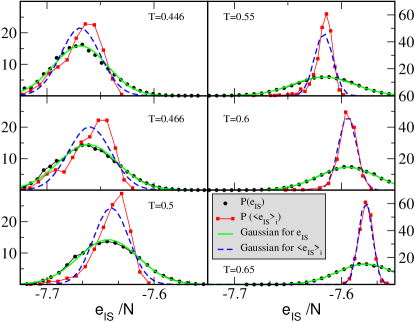
Figure 1: Probability distribution $P(e_{IS},T)$ of exploring an IS of depth $e_{IS}$ at temperature $T$. Black filled circles: equilibrium data for the N=155 system. Green full line: Gaussian distribution of variance $18$. The figure also shows, with red filled squares the distribution $P(<e_{IS}>_{i},T)$ (where $<e_{IS}>_{i}$ is not the instantaneous value but $e_{IS}$ averaged over time $t_{MSD=1}$ for the trajectory $i$ and with a blue dashed line a Gaussian distributions with the same variance as $P(<e_{IS}>_{i},T)$.

Next we attempt to associate each of the independent configurations to an $e_{IS}$ value characterizing the location of the system in the PEL and to a $D_{i}$ value characterizing its local diffusion coefficient. We further propagate each of the configurations for a time $t_{<MSD>=1}$, defined as the time at which the type-A particles mean square displacement (MSD), averaged over all trajectories and all $A$ particles, reaches one. Different trajectories show very different dynamical properties. As an example, Fig. 2-a represents the MSD, as a function of $t$ for two different trajectories at the same $T$. Each trajectory $i$ has a rather well defined diffusion coefficient $D_{i}$ which can be extracted from the slope of the MSD vs time. Fig. 2-b shows the $t$-evolution of $e_{IS}$ for the same two trajectories. The more mobile system is characterized by a larger and more fluctuating $e_{IS}$. Within $t_{<MSD>=1}$, the set of $e_{IS}$ values explored is far from covering the full range of values characteristic of that $T$. The system retains memory of the starting configurations and this behavior is enhanced at lower $T$. A quantification of the location of the $i$-configuration on the PEL can thus be provided by $<e_{IS}>_{i}$, defined as the value of $e_{IS}$ averaged over the time interval from zero to $t_{<MSD>=1}$.

Fig. 1 also show the probability distribution $P(<e_{IS}>_{i},T)$. While $P(e_{IS},T)$ are well approximated by a Gaussian distribution of average $<e_{IS}(T)>$ and constant variance (in agreement with Eq.1), $P(<e_{IS}>_{i})$ are symmetric and well modelled by a Gaussian only at high $T$. At low $T$ $P(<e_{IS}>_{i},T)$ becomes strongly asymmetric, and its variance increases on cooling. This originates in the different mobility of the system depending on the initial $e_{IS}$. Indeed, while systems with $e_{IS}$ associated to the high energy tail of $P(e_{IS},T)$ manage to explore different basins, systems in the low energy tail hardly lose memory of the initial configuration within $t_{<MSD>=1}$. In this respect, the observed asymmetry confirms that there is a strong coupling between $<e_{IS}>_{i}$ and $D_{i}$, which we now try to quantify.

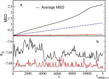
Figure 2: a) MSD as a function of time for two different equilibrated trajectories at the same thermodynamical state point ($T=0.446$, $\rho=1.2$). The MSD is here averaged over all type-$A$ particles of the system as well as over several starting times within the interval $0<t<t_{<MSD>=1}$. The dashed line represents the MSD averaged over all trajectories and it provides the definition of $t_{<MSD>=1}$. b) Inherent structure energies as a function of time for the same trajectories shown in a).

Fig. 3-a shows $D_{i}$ as a function of $<e_{IS}>_{i}$ at several $T$. Data from different $T$ overlap in a wide window of $e_{IS}$ values. Data show that the local diffusivity is function of $T$ not only via the $T$-dependence of $e_{IS}$ but also directly, since for each chosen $e_{IS}$ value, data for higher $T$ always lay above data at lower $T$. The fact that basins of the same depth are sampled at different $T$ allows us to evaluate the $T$ dependence of $D$ at fixed basin depth and sort out the relative contribution of $T$ and $e_{IS}$ to dynamics. To distinguish between the $T$ and $e_{IS}$ dependence of $D$ we hypothesize that the law relating these two quantities has the form:

$$D(e_{IS},T)=D_{\infty}e^{-\frac{f(e_{IS})}{T}},$$ (3)

a form compatible both with the idea of activated dynamics as well as with the Adam-Gibbs (AG) hypothesis $ln(D/D\infty)=\frac{-B}{TS_{conf}}$ (in which case $1/f(e_{IS})=S_{conf}(e_{IS})/B$), with $B$ being a coefficient related to the minimum size of a cooperatively rearranging region.

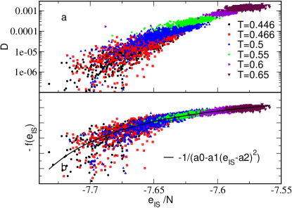
Figure 3: Diffusivity $D_{i}$ as a function of the corresponding average $<e_{IS}>_{i}$. Different symbols indicate the six different simulated $T$. b) $Tln(D(e_{IS},T)/D_{\infty})$ as a function of $e_{IS}$. The solid line represent the fitting function $-\frac{1}{a_{0}-a_{1}(e_{IS}-a_{2})^{2}}$.

According to Eq. 3, a plot of $Tln(D(e_{IS},T)/D_{\infty})$ should produce a collapse of all data, independently of $T$, onto a master curve which can be identified as $-f(e_{IS})$. Fig. 3-b confirms that indeed such a procedure generates an impressive scaling of the data. We note that, in this procedure, we use the value of $D_{\infty}=0.155$ obtain independently from high $T$ simulations. If the resulting $f(e_{IS})$ is interpreted according to activated models, one has to conclude that the height of the barriers increases significantly on cooling, diverging as the limiting $e_{IS}$ value $e_{K}=-7.81$ is approached, a result which appears to contradict, in the details, the analysis performed previously by Doliwa and Heuer heuernew . If $f(e_{IS})$ is interpreted according to the AG equation, then $1/f(e_{IS})$ has to be proportional to $S_{conf}(e_{IS})$, a quantity which has been previously calculated for this model using thermodynamic integration techniques skt99 ; sastry01 ; depablo .

The test between the two different estimates of $S_{conf}$ can be made even more stringent, if one realizes that, by fitting $f(e_{IS})$ according to the relation $f(e_{IS})=\frac{1}{a_{0}-a_{1}(e_{IS}-a_{2})^{2}}$ the fitting coefficient $a_{0}$, $a_{1}$ and $a_{2}$ can be associated, comparing with Eq. 2, to

$$a_{0}=(\alpha N)/B$$

$$a_{1}=1/(2\sigma^{2}B)$$

$$a_{2}=E_{0}$$ (4)

Interestingly enough, since $\sigma^{2}$ is known independently from the (T-independent) width of $P(e_{IS},T)$, $a_{1}$ provides $B$, $a_{0}$ $\alpha$ and $a_{2}$ provides $E_{0}$ (yielding respectively $B=1.85$,$\alpha=0.78$,$E_{0}=-1140$). Thus, an estimate of $S_{conf}$ in absolute units is provided by the fit parameters. The comparison between $S_{conf}$ obtained via thermodynamic integration (from Ref.skt99 ) and $S_{conf}$ obtained here from $f(e_{IS})$ is shown in Fig. 4. The agreement between the two independent estimates of $S_{conf}$ confirms the previously observed possibility of describing the dynamics in this model according to the AG equationsastry01 and to the interpretation of the landscape basins as stateswolynes .

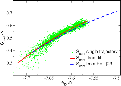
Figure 4: Comparison between $S_{conf}$ evaluated from Eq.  2 and  4 (solid line), and $S_{conf}$ from skt99 (dashed line). The symbols are the values obtained for each trajectory $i$.

The combined use of the PEL thermodynamic formalism and of the relation between thermodynamic and dynamics provided by Eq. 3 makes it possible to evaluate the $T$-dependence of $D$ for the present model, — independently from the interpretation in terms of activated processes with $e_{IS}$ dependent barrier or in term of AG — according to

$$D(T)=\int D(e_{IS},T)P(e_{IS},T)de_{IS}.$$ (5)

Fig. 5 shows $D$ evaluated directly from the MSD long time limit and from Eq. 5. The agreement between the two sets of independent data strongly support the possibility of representing $D$ as a sum over the local diffusivity of different parts of the landscape. This representation is very intriguing and offers an alternative way, within the landscape framework, to look at dynamic heterogeneities, which have been widely studied theoretically, in simulations and experiments in recent years stillingerandh ; tarjus ; harro ; scg ; onuki ; mik ; gc ; cicerone; Chang; weeks ; kegel ; ediger ; bordat ; szamel . Indeed, the nonlinear relation between $D$ and $e_{IS}$ (Eq. 3) implies that at low $T$, in equilibrium, the system can be represented by coexisting regions in space with very different local mobility. As seen in Fig. 3, at the lowest investigated $T$, the $D_{i}$ values cover about three different orders of magnitude. It is important to stress that the inhomogeneities in the dynamics are, in the present case, strongly associated to structural properties and in particular to the depth of the lS locally sampled.

This extremely wide distribution of $D_{i}$ values suggests also a possible explanation of the $T$-dependence of the product $D\tau_{\alpha}$ upon supercooling, analyzed with reference to heterogeneous dynamics in, e. g. stillingerandh ; tarjus ; onuki ; mik ; gc , along the lines proposed in Ref. stillingerandh . Indeed, when a distribution is wide, the mean and the inverse of the average of its inverse can be rather different, since they weigh different parts of the distribution. To evaluate this effect in the present case we compare in Fig. 5 the $T$ dependence of the product $<D><1/D>$. On cooling, the product starts to deviate from one, consistently with the observations for the model liquid studied here that the product $D\eta/T$ bordat and $D\tau_{\alpha}$szamel starts to increase on cooling.

In summary, by considering large numbers of realizations of the trajectory of a small system of particles, we have shown that the dependence of the diffusion coefficients for each such trajectory on the depth of the potential energy minima explored can be extracted in a model-free manner, and that the average diffusion coefficient for the system can be estimated as a sum over contributions of the sampled basins, establishing a connection between thermodynamics and dynamics in the potential energy landscape framework. We provide evidence that the observed non-linearity in the relation between local diffusion and basin depth is responsible for the peculiar dynamic behavior observed in supercooled states and provide an interpretation within the energy landscape picture for the presence of dynamic heterogeneities.

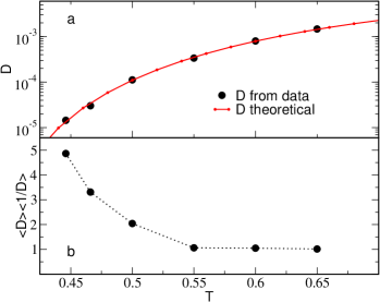
Figure 5: a) Diffusivity constant as from data compared with the diffusivity constant evaluated from Eq. 5. b) Product $<D><1/D>$ form data as a function of $T$. The dashed line is a guide for the eye.

We acknowledge support from MIUR-FIRM. S. Sastry thanks the University of Roma for hospitality.

References

- (1) Kurt Binder and Walter Kob Glassy Materials and Disordered Solids: An Introduction to their Statistical Mechanics World Scientific, Singapore (2005).
- (2) P. G. Debenedetti and F. H. Stillinger, Nature 410, 259 (2001).
- (3) F. H. Stillinger and T. A. Weber, Phys. Rev. A 25, 978 (1982); Science 225, 983 (1984); F. H. Stillinger, ibid. 267, 1935 (1995).
- (4) F. Sciortino, J. Stat. Mech. P05015 (2005).
- (5) S. Sastry, Nature 409, 164 (2001).
- (6) S. Büchner, and A. Heuer, Phys. Rev. E 60, 6507 (1999).
- (7) S. Mossa et al., Phys. Rev. E 65, 0412-05-1 (2002).
- (8) E. La Nave et al., Physical Review E 68, 032103 (2003).
- (9) I. Saika-Voivod , P.H. Poole and F. Sciortino, Nature 412, 514 (2001).
- (10) A. J. Moreno et al., Phys. Rev. Lett. 95, 157802 (2005).
- (11) W. Kob and H. C. Andersen, Phys. Rev. Lett. 73, 1376 (1994).
- (12) We simulate a system of 155 particles in a volume corresponding to a reduced density of 1.2 . The system is a binary mixture of particles A ( %) and B ( %). The interaction potential (including the cut-off values) coincides with the one introduced in Ref. kobandersen . Units of energy and length are defined by the and parameters of the Lennard Jones interaction potential and the unit of mass the mass of the A particles. Temperatures are expressed in units of . Determination of the IS energy has been performed using a standard conjugate-gradient minimization algorithm.
- (13) T. A. Weber and F. H. Stillinger, Phys. Rev. B. 31, 1954 (1985).
- (14) T. Keyes, J. Chem. Phys. 101, 5081 (1994).
- (15) E. La Nave, H.E. Stanley and F. Sciortino, Phys. Rev. Lett. 88, 035501 (2002).
- (16) L. Angelani et al., Phys. Rev. Lett. 85, 5356 (2000).
- (17) K. Broderix, K.K. Bhattacharya, A. Cavagna, A. Zippelius and I. Giardina Phys. Rev. Lett. 85, 5360 (2000).
- (18) A. Scala et al., Nature 406, 166 (2000).
- (19) B. Doliwa and A. Heuer, Phys. Rev. Lett. 91, 235501 (2003).
- (20) T. B. Schrøder, S. Sastry, J. C. Dyre and S. C. Glotzer, J. Chem. Phys. 112, 9834 (2000).
- (21) A. Widmer-Cooper P. Harrowell and H. Fynewever, P. Harrowell Phys. Rev. Lett, 93, 135701 (2004).
- (22) I. Saika-Voivod and F. Sciortino, Phys. Rev. E 70, 041202 (2004).
- (23) F. Sciortino, W. Kob and P. Tartaglia, Phys. Rev Lett. 83, 3214 (1999).
- (24) R. Faller and J. de Pablo, J. Chem. Phys., 119, 4405 (2003).
- (25) X. Xia and P. G. Wolynes, PNAS 97, 2990 (1999).
- (26) J. A. Hodgdon, and F. H. Stillinger, Phys. Rev. E. 48 207 (1993).
- (27) G. Tarjus and D. Kivelson, J. Chem. Phys. 103, 3071 (1995).
- (28) D. N. Perera and P. Harrowell, Phys. Rev. E 54, 1652 (1996).
- (29) W. Kob, C. Donati, S. J. Plimpton, P. H. Poole and S. C. Glotzer, Phys. Rev. Lett. 79 2827 (1997).
- (30) R. Yamamoto and A. Onuki, Phys. Rev. Lett. 81, 4915 (1998)
- (31) M. Dzugutov, S. I. Simdyankin and F. H. M. Zetterling, Phys. Rev. Lett. 89, 195701 (2002).
- (32) Y-J. Jung, J. P. Garrahan and D. Chandler, Phys. Rev. E. 69 061205 (2004). M. T. Cicerone, F. Blackburn, and M. D. Ediger, J. Chem. Phys., 102, 471 (1995). I. Chang and H. Sillescu, J. Phys. Chem. B 101, 8794 (1997).
- (33) E. R. Weeks, J. C. Crocker, A. C. Levitt, A. Schofield and D. A. Weitz, Science 287 627 (2000).
- (34) W. K. Kegel and A. van Blaaderen, Science 287 290 (2000).
- (35) M. D. Ediger, Annu. Rev. Phys. Chem. 51 99 (2000).
- (36) P. Bordat, et al, J. Phys.: Cond. Mat. 15 5397 (2003).
- (37) E. Flenner and G. Szamel, Phys. Rev. E 72, 031508 (2005).