A continuous-time solver for quantum impurity models

Abstract

We present a new continuous time solver for quantum impurity models such as those relevant to dynamical mean field theory. It is based on a stochastic sampling of a perturbation expansion in the impurity-bath hybridization parameter. Comparisons to quantum Monte Carlo and exact diagonalization calculations confirm the accuracy of the new approach, which allows very efficient simulations even at low temperatures and for strong interactions. As examples of the power of the method we present results for the temperature dependence of the kinetic energy and the free energy, enabling an accurate location of the temperature-driven metal-insulator transition.

Numerical computation of dynamical properties of strongly correlated fermion systems is one of the fundamental challenges in condensed matter physics. The exponential growth of the Hilbert space renders exact diagonalizations impossible except for very small systems exactdiag . When applied directly to lattice models, auxiliary field Monte Carlo methods encounter severe difficulties with the fermionic sign problem auxiliary_problem . The density matrix reormalization group White92 is powerful for extracting ground state properties of one dimensional systems, but extensions to higher dimensions and dynamics have proven difficult. Over the last decade, a promising new “dynamical mean field” (DMFT) approach has been developed Mueller-Hartmann89 ; Metzner89 ; Georges92 . As shown by Georges, Kotliar and other workers Georges92 ; Georges96 ; Maier05 , if the momentum dependence of the self-energy is neglected, $\Sigma(p,\omega)\rightarrow\Sigma(\omega)$, then the solution of the lattice model may be obtained from the solution of a quantum impurity model plus a self-consistency condition.

A quantum impurity model represents an atom or molecule embedded in a host medium; in addition to their relevance to DMFT calculations these models are of intrinsic interest and important to nano-science as representations of single-molecule conductors. A quantum impurity model consists of a set of levels $a$ (with creation operators $\psi_{a}^{\dagger}$), populated by electrons which interact via general four-fermion interactions $U^{abcd}$ (for example density-density or spin exchange terms). The levels $a$ are hybridized to electronic continua (“bath orbitals”) representing the degrees of freedom of the host material. These bath degrees of freedom may be integrated out, and the impurity model specified by a partition function $Z=\text{Tr}T_{\tau}e^{-S}$ with effective action $S=S_{F}+S_{\text{loc}}$, where

$$S_{F} = -\int_{0}^{\beta}d\tau d\tau^{\prime}\psi_{a}^{\phantom{\dagger}}(\tau)F_{a}(\tau-\tau^{\prime})\psi_{a}^{\dagger}(\tau^{\prime}),$$ (1)

$$S_{\text{loc}} = -\int_{0}^{\beta}d\tau(\epsilon^{ab}\psi_{a}^{\dagger}\psi_{b}^{\phantom{\dagger}}-U^{abcd}\psi^{\dagger}_{a}\psi^{\dagger}_{b}\psi^{\phantom{\dagger}}_{c}\psi^{\phantom{\dagger}}_{d}).$$ (2)

The function $F$ is determined by the hybridization and bath density of states. It describes transitions from the impurity into the bath and back and is related to the mean field function $G_{0}^{-1}$ Georges96 by $G_{0}^{-1}(i\omega)=i\omega+\mu-F(-i\omega)$. A solution of the quantum impurity model amounts to evaluating the Green functions $G(\tau)=-\langle T_{\tau}\psi(\tau)\psi^{\dagger}(0)\rangle$ for given $F$, $\epsilon$ and $U$. The dynamical mean field procedure involves a self-consistent determination of the hybridization function $F$, in which the computation of $G$ is time critical Georges96 .

Perhaps the most commonly used technique is the Hirsch-Fye method Hirsch86 , in which a (discrete) Hubbard-Stratonovich transformation is used to decouple the interaction part, leading to determinants which give the weights associated with the configurations of the auxiliary fields, which are then sampled by a Monte Carlo procedure. The method requires a discretization of the imaginary time interval $[0,\beta]$ into $N$ equal slices and the evaluation of determinants of $N\times N$ matrices. At low temperatures and strong correlations, the Green functions have a highly non-uniform time dependence, dropping very steeply near the edge points $\tau=0,\beta$, and varying more slowly in between. The rapid drop means that a very large $N$ ($\sim 5U\beta$) is required, limiting the utility of the algorithm for physically relevant temperatures. Furthermore, useful decouplings of the general interactions of multiorbital models are lacking. Another approach is an exact diagonalization method Caffarel94 ; Toschi05 in which the continuum of energies in the impurity model is replaced by a discrete set of levels. This method suffers from systematic errors associated with the discrete level spacing, and becomes impractical in the multiorbital case because of the rapid growth of the Hilbert space.

In this paper we present a new, continuous time approach which resolves many of these issues. The idea, introduced in the context of bosonic field theories by Prokof’ev et al. Svistunov96 , is to define a formal perturbation expansion for the partition function $Z$. Certain collections of terms in this series are then sampled by a Monte Carlo procedure. In important prior work, Rubtsov and co-workers Rubtsov05 performed such a stochastic evaluation by expanding in the interaction term. In this paper we show how to formulate a determinental Monte Carlo algorithm by expanding in the hybridization term $S_{F}$ while treating the interactions exactly. This strong-coupling approach becomes particularly powerful at the strong interactions characteristic of systems of present day interest (such as high-$T_{c}$ cuprates), because the perturbation order actually decreases with increasing $U$. Our method allows access to low enough temperatures that both ground state properties and the leading temperature dependencies may be determined, even at very strong couplings, providing new information unavailable by other methods.

We illustrate the procedure first for noninteracting spinless fermions, and then proceed to the one-orbital Hubbard model, reserving a general discussion for a future publication Werner06b . Because the spinless fermion model is diagonal in the occupation number basis, we have for $Z^{F}\equiv Z(\mu=0,U=0,\sigma)$

$$Z^{F}=2+\sum_{k=1}^{\infty}\int_{0}^{\beta}d\tau_{1}^{s}\int_{\tau_{1}^{s}}^{\beta}d\tau_{1}^{e}\int_{\tau_{1}^{e}}^{\beta}d\tau_{2}^{s}\int_{\tau_{2}^{s}}^{\beta}d\tau_{2}^{e}\ldots$$

$$\ldots\int_{\tau_{k-1}^{e}}^{\beta}d\tau_{k}^{s}\int_{\tau_{k}^{s}}^{\circ\tau_{1}^{s}}d\tau_{k}^{e}Z^{F}_{k}(\tau_{1}^{s},\tau_{1}^{e};\tau_{2}^{s},\tau_{2}^{e};\ldots;\tau_{k}^{s},\tau_{k}^{e}),$$ (3)

with $Z^{F}_{k}(\tau_{1}^{s},\tau_{1}^{e};\tau_{2}^{s},\tau_{2}^{e};\ldots;\tau_{k}^{s},\tau_{k}^{e})$ denoting the collection of $k!$ diagrams containing $k$ segments of occupied fermion states, with starting point $\tau_{i}^{s}$ and end point $\tau_{i}^{e}$, $i=1,\ldots,k$. We view the interval $[0,\beta]$ as a circle and take care of the trace over occupation number states by including diagrams in which the last fermion line winds around the circle. This is denoted by an upper integral bound $\circ\tau$. An illustration of these diagrams for $k=3$ is shown in Fig. 1. Each end point $\tau_{m}^{e}$ is connected to a starting point $\tau_{n}^{s}$ by a dashed line representing $F(\tau_{m}^{e}-\tau_{n}^{s})$. The collection of diagrams evaluates to

$$Z^{F}_{k}(\tau_{1}^{s},\tau_{1}^{e};\tau_{2}^{s},\tau_{2}^{e};\ldots;\tau_{k}^{s},\tau_{k}^{e})=\det M^{-1}\delta_{\tau_{1}^{s}}^{\tau_{k}^{e}},$$ (4)

$$(M^{-1})_{m,n}=F(\tau_{m}^{e}-\tau_{n}^{s}),$$ (5)

with $\delta_{\tau_{1}^{s}}^{\tau_{k}^{e}}=-1$ if $\tau_{k}^{e}<\tau_{1}^{s}$ (the last segment winds around the circle ) and $+1$ otherwise. One also has to sample the “full line” and the “empty line” states, corresponding to 1 or 0 particle in the whole interval $0\leq\tau<\beta$. We use three types of Monte Carlo updates: (i) insertion and removal of a segment, (ii) insertion and removal of an anti-segment, and (iii) shift of the segment end point. The first two are required for ergodicity and the third enhances the sampling efficiency.

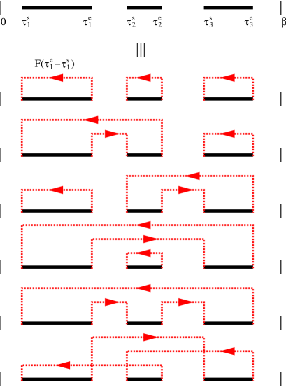
Figure 1: Illustration of $Z^{F}_{3}(\tau_{1}^{s},\tau_{1}^{e};\tau_{2}^{s},\tau_{2}^{e};\tau_{3}^{s},\tau_{3}^{e})$ in terms of diagrams. A full line corresponds to an occupied fermion state. Each end point $\tau_{m}^{e}$ of a segment is connected to a starting point $\tau_{n}^{s}$ by a dashed line representing $F(\tau_{m}^{e}-\tau_{n}^{s})$. The combined weight of the diagrams can be expressed as a determinant.

Combining the $k!$ diagrams into a determinant is essential. Some diagrams have negative weight and a “worm”-type algorithm which sampled individual diagrams would run into a bad sign problem. Yet we found in all of our computations that the determinant remains positive.

Suppose we start with a collection of segments $s_{k}=(\tau_{1}^{s},\tau_{1}^{e};\tau_{2}^{s},\tau_{2}^{e};\ldots;\tau_{k}^{s},\tau_{k}^{e})$ and want to insert a new segment $\tilde{s}$ at a randomly chosen $\tilde{\tau}^{s}$. If $\tilde{\tau}^{s}$ happens to lie on a segment of $s_{k}$, the move to the new configuration $s_{k+1}=s_{k}+\tilde{s}$ is rejected, otherwise it has to satisfy a detailed balance condition. If the length $\tilde{l}$ of the new segment is chosen randomly in the interval $[0,l_{\text{max}}]$, with $l_{\text{max}}$ determined by $\tilde{\tau}^{s}$ and the collection $s_{k}$ of existing segments, and we propose to remove this new segment in the new configuration $s_{k+1}$ with probability $1/(k+1)$, the condition is

$$\frac{p_{\text{ins}}(s_{\text{new}})}{p_{\text{rem}}(s_{\text{new}})}= \frac{Z^{F}_{k+1}(s_{k+1})}{Z^{F}_{k}(s_{k})}\frac{\beta l_{\text{max}}}{k+1}e^{\tilde{l}\mu}.$$ (6)

The result for anti-segments is similar and for shift updates from a configuration $s$ to a configuration $\tilde{s}$ (changing the length of some segment from $l$ to a randomly chosen $\tilde{l}\in[0,l_{\text{max}}]$) one obtains

$$\frac{p(s\rightarrow\tilde{s})}{p(\tilde{s}\rightarrow s)}= \frac{Z^{F}_{k}(\tilde{s})}{Z^{F}_{k}(s)}e^{(\tilde{l}-l)\mu}.$$ (7)

Figure 2: Green functions for $n=1$, $U/t=3.5\sqrt{2}$, $\beta t=400,200,31.4$ and $20$. Lines without symbols (upper and right axes) show $G(\tau)$ on a semi-log scale over the wide time interval $[\beta/2,\beta]$ revealing marked differences between metallic ($\beta t=200,400$) and insulating ($\beta t=20,31.4$) solutions. Lines with symbols (lower and left axes) show the same data on a linear scale in the very narrow $\tau$ range $[0,\beta/2000]$, revealing the accurate representation of the rapid drop of $G(\tau)$.

A procedure analogous to that in Ref. Rubtsov05 is used to calculate the determinant ratios and the new enlarged (reduced) matrices in a time $O(k^{2})$. We store and manipulate $M$, the inverse of Eq. (5), because $M$ allows easy access to the determinant ratios in Eqs. (6) and (7) and is required for measuring the Green function, since

$$G(\tau) =\Big{\langle}\frac{1}{\beta}\sum_{i=1}^{k}\sum_{j=1}^{k}M_{j,i}\Delta(\tau,\tau_{i}^{e}-\tau_{j}^{s})\Big{\rangle},$$ (8)

$$\Delta(\tau,\tau^{\prime}) =\left\{\begin{array}[]{ll}\delta(\tau-\tau^{\prime})&\tau^{\prime}>0\\ -\delta(\tau-\tau^{\prime}-\beta)&\tau^{\prime}<0\end{array}\right..\hskip 14.22636pt$$ (11)

The end points $G(0)$ and $G(\beta)$ can be measured accurately from the average total length of the segments.

In the form given here, the algorithm generalizes straightforwardly to any model with interaction terms which are diagonal in an occupation number basis (for models with exchange, see Ref. Werner06b ). One simply introduces one collection of segments for each spin/orbital state, and the weight of a configuration now also depends on the segment overlap. For example, in the one-orbital Hubbard model with on-site interaction $U$, there is one collection of segments for spin up and one for spin down, while in Eqs. (6) and (7) one has to add a factor $\exp(-\delta_{\text{ov}}U)$ on the right hand side, where $\delta_{\text{ov}}$ denotes the change in overlap between up and down segments.

We have used the new method to study the paramagnetic phase of the Hubbard model with semicircular density of states of bandwidth $4t$, for interactions of the order of the Mott critical value $U_{c2}$ and temperatures as low as $\beta t=400$. For this model the self-consistency condition reduces to $F(\tau)=t^{2}G(-\tau)$. Simulations for temperatures down to $\beta t\approx 50$ can be run on a laptop. For calculations at $\beta t=400$, we typically used 10 CPU hours for each iteration in order to accurately resolve the short- and long-time behavior.

Figure 2 shows the impurity model Green function for $U/t=3.5\sqrt{2}$, $\beta t=20$, 31.4, 200 and $400$ and $n=1$ (half filling). The lower two temperatures are out of reach of the Hirsch-Fye algorithm. We collected the data on a grid of $10^{4}$ points for $\beta t=200,400$ and $10^{3}$ points for $\beta t=20,31.4$. The lines with symbols show that the method accurately captures the steep short-time drop of $G$; the lines without symbols demonstrate clearly the difference in long-time behavior between the insulating (high-$T$) and metallic (low-$T$) solutions.

Figure 3: Probability $p(k)$ for a configuration with $k$ segments plotted for different interaction strengths $U/t$ for $\beta t=100$ and half-filling. The peak position shifts to lower values of $k$ as $U/t$ is increased. The inset compares the scaling of the matrix size with $U$ to Hirsch-Fye ($\approx 5\beta U$) and the method of Ref. Rubtsov05 ($\approx 0.5\beta U$).

Despite the almost perfect resolution, the typical size, $k$, of the matices, $M$, which are generated during the simulation remains reasonable even at low temperatures. This property explains the superior performance of the strong-coupling expansion method. Figure 3 shows the probability distribution $p(k)$ for $\beta t=100$ and different values of the interaction strength. While the peak value of the distribution is proportional to $\beta$, it shifts to lower order as the interaction strength is increased, in contrast to Hirsch-Fye or the method of Ref. Rubtsov05 , where the matrix size scales approximately as $5\beta U$ and $0.5\beta U$, respectively. The inset of Fig. 3 shows that the linear size of the matrix in our method can easily be a factor 100 smaller than in a Hirsch-Fye calculation or a factor $10$ smaller than in the weak-coupling approach of Ref. Rubtsov05 . The cubic scaling of the computational effort with matrix size implies a dramatically improved efficiency at couplings of the order of the Mott critical value, making low $T$ behavior accessible.

Figure 4: Kinetic energy obtained using the indicated impurity solvers plotted as a function of temperature for $U/t=4$ and $U/t=3.5\sqrt{2}\approx 4.95$. The former value corresponds to a metallic phase, while for $U/t=3.5\sqrt{2}$, the system undergoes a metal-insulator transition.

To verify the accuracy of the method we show in Fig. 4 the kinetic energy $K=2t^{2}\int_{0}^{\beta}d\tau G(\tau)G(-\tau)$ obtained via the new approach, the exact diagonalization method Capone06 , and the Hirsch-Fye method. The results are plotted against $T^{2}$ to show that the theoretically expected Fermi liquid result can be obtained even when the characteristic energy scales are very low. The new algorithm displays the metal-insulator transition clearly, agrees perfectly with exact diagonalization results, and is consistent with the Hirsch-Fye data at elevated temperatures.

Figure 4 shows a discontinuity arising from the instability of the metallic solution as the temperature is increased above a certain value ($T/t\approx 0.026$ at $U/t=4.95$). The instability implies the existence of a first order metal-insulator transition, but strictly speaking it is a spinodal point. To further demonstrate the power of the method we locate the true phase boundary by constructing the free energy of the metallic state. We compute the total internal energy per site $E(T)=K(T)+U\langle n_{\uparrow}n_{\downarrow}\rangle$, from which we obtain the specific heat $C(T)=dE(T)/dT$ and hence the entropy $S(T)=\int_{0}^{T}dT^{\prime}(C(T^{\prime})/T^{\prime})$. We compare this to the free energy of the paramagnetic insulating state for which $E(T)$ has negligible $T$-dependence because of the gap, but the entropic contribution is $-T\ln 2$. Results are illustrated in Fig. 5 for $U/t=5.3$, where the interaction is so large that exact diagonalization data in the relevant $T$ regime are not available. The jump in the kinetic energy is clearly seen to be a spinodal effect, occuring at a higher temperature ($T\approx 0.011t$) than the $T_{c}=0.00685(4)t$ at which the free energies cross. The latent heat of this metal-insulator transition is $T_{c}(S_{\text{met}}(T_{c})-S_{\text{ins}})=0.00250(5)t$.

Figure 5: Points: Kinetic energy as a function of temperature for $U/t=5.3$. Solid line with error estimates as dotted lines: free energy of the metallic state. Dashed line: free energy of the insulating state. Inset: quadratic $T$-dependence of the total energy.

In conclusion, we have developed a continuous-time impurity solver, based on a stochastic evaluation of an expansion in the hybridization. The new approach, which (even away from half-filling) does not appear to suffer from a sign problem, is much more efficient at intermediate to strong couplings than other available methods. It allows to simulate the Hubbard model at previously inaccessible temperatures, permitting direct access to the asymptotic low energy physics, for example allowing the computation of the latent heat across the metal-insulator transition. The algorithm opens up for systematic study the low temperature properties of strongly interacting quantum models relevant to transition metal oxides, actinides and other correlated electron materials.

PW, AC and AJM acknowledge support from NSF DMR 0431350, and LdM from the Columbia-Science Po “Alliance” program. We thank N. Prokof’ev, A. Rubtsov and T. Pruschke for stimulating discussions. The continuous-time calculations were performed on the Hreidar cluster at ETH Zürich, using the ALPS library ALPS .

References

- (1) E. Dagotto, Int. J. Mod. Phys. B 5, 77 (1991).
- (2) E. Y. Loh Jr. et. al., Phys. Rev. B 41, 9301 (1990).
- (3) S. R. White, Phys. Rev. Lett. 69, 2863 (1992).
- (4) E. Müller-Hartmann, Z. Phys. B74 507 (1989).
- (5) M. Metzner and D. Vollhard, Phys. Rev. Lett. 62, 324 (1989).
- (6) A. Georges and G. Kotliar Phys. Rev. B 45, 6479 (1992).
- (7) A. Georges et al., Rev. Mod. Phys. 68, 13 (1996).
- (8) T. Maier et al., Rev. Mod. Phys. 77, 1027 (2005).
- (9) J. E. Hirsch and R. M. Fye, Phys. Rev. Lett. 56, 2521 (1986).
- (10) M. Caffarel and W. Krauth, Phys. Rev. Lett. 72,1545 (1994).
- (11) A. Toschi et al., Phys. Rev. Lett. 95, 097002 (2005).
- (12) N. V. Prokof’ev et al., JETP Lett. 64, 911 (1996).
- (13) A. N. Rubtsov et al., Phys. Rev. B 72, 035122 (2005).
- (14) P. Werner and A. J. Millis, cond-mat/0607136.
- (15) M. Capone, L. de’ Medici, and A. Georges, cond-mat/0512484.
- (16) M. Troyer et al., Lecture Notes in Computer Science 1505, 191 (1998); F. Alet et al., J. Phys. Soc. Jpn. Suppl. 74, 30 (2005); http://alps.comp-phys.org/ .