Entropy and Correlation Functions of a Driven Quantum Spin Chain

Abstract

We present an exact solution for a quantum spin chain driven through its critical points. Our approach is based on a many-body generalization of the Landau-Zener transition theory, applied to fermionized spin Hamiltonian. The resulting nonequilibrium state of the system, while being a pure quantum state, has local properties of a mixed state characterized by finite entropy density associated with Kibble-Zurek defects. The entropy, as well as the finite spin correlation length, are functions of the rate of sweep through the critical point. We analyze the anisotropic XY spin $1/2$ model evolved with a full many-body evolution operator. With the help of Toeplitz determinants calculus, we obtain an exact form of correlation functions. The properties of the evolved system undergo an abrupt change at a certain critical sweep rate, signaling formation of ordered domains. We link this phenomenon to the behavior of complex singularities of the Toeplitz generating function.

I Introduction

Recent advances in the studies of ultracold atoms trapped in optical lattices have opened a new arena of investigation of nonequilibrium strongly correlated quantum systems Greiner et al. (2002); Jacksch et al. (1998). These new opportunities are epitomized by the pioneering experiments on tunable Mott insulator-to-superfluid quantum phase transition, observed by manipulation of the optical lattice potential in 3d Greiner et al. (2002) and 1d Stöferle et al. (2004) systems. The highly controllable environment and long coherence times of these systems provide new framework for investigation of nonequilibrium dynamics of quantum critical phenomena Clark and Jaksch (2004); Dziarmaga et al. (2002); Sengupta et al. (2004).

One interesting question arising in this framework has to do with the properties of defects produced by sweeping through a critical point. For the phase transitions occurring at finite temperature the defect production is described by Kibble-Zurek (KZ) theory Kibble (1976); Zurek (1985). This theory, which initially was applied to topological defects left behind cosmological phase transitions, and only later found its way in condensed matter physics, estimates the correlation length in the ordered state using a causality argument. The correlation length serves as a measure of the size of the ordered domains and of typical separation between defects. Defect production was probed in recent experiments employing superfluid ${}^{3}{\rm He}$ Ruutu et al. (1996); Bauerle et al. (1996) and superconducting Josephson junctions Carmi et al. (2000).

Phase transitions in cold atom systems are characterized by a high degree of coherence, which makes the dynamics near the critical point essentially non-dissipative. The theory of defect production in this situation has to be modified to account for coherent dynamics. Defect production in quantum dynamics can be studied using integrable 1d spin models. The 1d spin models with varying coupling constants provide a template for many quantum phenomena. Realizations of such models have been proposed recently in 1d qubit chainsLevitov et al. (2001) and optical latticesDuan et al. (2003). The models of quantum spin quench dynamics resulting from an abrupt change of coupling constant which takes the system across the phase boundary, were considered in Refs.Sengupta et al. (2004); Calabrese and Cardy (2005). The quench dynamics, while providing useful insight, do not describe the situation of a continuous sweep across the transition, which is addressed in the present work.

Besides defect production rate and density, there is an interesting question of the entropy associated with the defects. Naively, it may seem that the entropy cannot be produced at zero temperature by a system evolving unitarily in a pure state. However, if the evolved state is sufficiently complex, it may look entropic from a local point of view, i.e. if observed in a volume much smaller than the total system size. As we shall see, this is precisely the case in this problem.

In the present article we study time evolution of a many-body system which is swept at a constant speed through its quantum critical point. With the help of an exactly solvable 1d quantum spin model with a time-dependent Hamiltonian we explore how the time evolution across the critical point manifests itself in the many-body effects and spin correlation functions. In particular, we analyze the relation between the sweep speed and spatial spin correlations, providing an extension of KZ scenario to the quantum critical point regime. Our analytical results are in agreement with recent numerical study of this problem, reported in Ref.Zurek et al. (2005).

Our approach is based on a many-body generalization of the Landau-Zener (LZ) transition theory. In this work we focus on the anisotropic XY spin $1/2$ chain with time-dependent couplings. We consider unitary evolution of the system, initially in the ground state, which crosses its equilibrium critical points. Since the Hamiltonian of the fermionized spin chain is quadratic, the evolution of the many-body state can be expressed with the help of a Bogoliubov transformation through a suitable set of the $2\times 2$ evolution problems of LZ form, one for each fermion momentum value.

Our analysis reveals that the evolved system state has a number of interesting characteristics. Firstly, despite being in a pure quantum state in a global sense, its local properties are identical to those of a system in a mixed state, characterized by finite effective temperature and entropy density. Although the finite entropy property of a pure state may seem counterintuitive, it naturally arises in the description of local properties, such as correlation functions. We shall see that the origin of finite entropy can be traced to coarse-graining in momentum space. On a more intuitive level, the system pure state can described as a superposition of different configurations of ordered domains with uniform magnetization. However, the coherence of amplitudes associated with different domain arrangements cannot be detected locally without having access to the entire set of variables in the system, which leads to an apparent mixed state and finite entropy.

Secondly, the transition from the adiabatic to non-adiabatic regime in the LZ problem, taken as a function of the sweep rate, depends on the momentum value of the fermionic mode. The characteristic crossover momentum can be associated with the inverse correlation length $\ell$ in the KZ picture, corresponding to typical domain size. This approach yields a scaling relation between the correlation length and the sweep speed, $\ell\propto v^{-1/2}$. This relation, obtained directly from the analysis of the many-body evolution operator, agrees with the KZ causality argument prediction.

Lastly, due to a simple product structure of the evolved state, the correlation functions can be obtained in a closed, exact form with the help of the theory of Toeplitz determinants. The correlation functions exhibit a crossover from monotonically decreasing behavior at fast sweep speed, $e^{-r/\ell}$, to an oscillatory behavior at a slow speed, $e^{-r/\ell}\cos(\omega r-\varphi)$. The oscillatory behavior, which appears abruptly below certain sweep speed value, corresponds to alternate magnetization signs in neighboring ordered domains (see Fig. 1). The spatial period $2\pi/\omega$ gives characteristic domain size. The parameters $\ell$, $\omega$ and $\varphi$ exhibit a singularity at the critical sweep speed, which is analyzed and explained in the Toeplitz determinant framework via evolution of zeroes of the generating function in a complex plane.

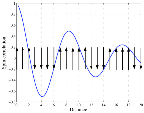
Figure 1: Spin correlation function schematic position dependence for slow sweep speed and corresponding typical arrangement of Kibble-Zurek domains. The correlation length and oscillation period are controlled by domain size.

The plan of this article is as follows. We start with analyzing the full many-body evolution operator of the XY spin chain with the help of Jordan-Wigner fermionization and reduction to the LZ transition problem in each fermion momentum subspace (Sec. II). Next, in Sec. IV, we show that in a macroscopic system (number of sites $N\to\infty$), a non-equilibrium steady state (NESS) emerges at late times. This is a mixed state characterized by a density matrix with finite entropy which depends on the sweep speed. The state of a mixed character appears due to decoherence intrinsic to the many-body LZ process, without any external decoherence effects. Technically, the mixed state arises as a result of taking the large $N$ limit in the correlation functions for spins separated by distances much less than the system size, $r\ll N$. This procedure allows to eliminate the rapidly oscillating terms in the correlation functions, which would disappear in a real system as a result of physical decoherence processes, even if the latter are extremely weak. The entropy of NESS is analyzed in Sec. V.

The density matrix description of NESS is subsequently used in Secs. VI and VIII to characterize ordering and analyze correlation functions. The method employed in analytic calculation uses some results from the theory of Toeplitz determinants which are reviewed in Appendix A. We obtain the asymptotics of equal-time spin correlators in the NESS which have non-trivial crossover behavior as a function of the sweep rate. Both numerical and analytical results are presented, compared, and found to be in agreement.

II Spin Chain Dynamics

In this section, we consider a quantum XY spin $1/2$ chain in time-dependent transverse field, described by the Hamiltonian

$${\cal H}(t) = -\frac{1}{2}\sum_{x=1}^{N}\left[J_{1}\sigma_{x}^{1}\sigma_{x+1}^{1}+J_{2}\sigma_{x}^{2}\sigma_{x+1}^{2}-h(t)\sigma_{x}^{3}\right]$$

where $N$ is the number of sites. The anisotropic coupling values are

$$J_{1}=J(1+\gamma)/2,\quad J_{2}=J(1-\gamma)/2,\quad h(t)=vt$$ (2.1)

Here $J=\frac{1}{2}(J_{1}+J_{2})$ is the average coupling and $\gamma=(J_{1}-J_{2})/(J_{1}+J_{2})$ is the anisotropy parameter. Note that the values $\gamma=0,\pm 1$ describe the isotropic XY model and the Ising model, respectively. (Without loss of generality, we assume $J>0$.)

In this article, the problem (II) is considered with periodic boundary conditions, i.e. $x=N+1$ is identified with $x=1$. Other choices, such as open boundary conditions, are possible. While the properties of interest in the large $N$ limit will be insensitive to the form of boundary conditions, periodic boundary conditions will make the intermediate steps of calculations more transparent.

The time-dependent transverse field $h(t)$ defines the evolution in the equilibrium system phase space which starts from and ends at the state in which the external field $h(t)$ is much larger than the couplings $J_{1,2}$ (Fig.2). Thus in the asymptotic ground states at $t\to\pm\infty$ the spins are fully polarized: $\psi^{(0)}_{-\infty}=(...\downarrow\downarrow\downarrow\downarrow...)$ and $\psi^{(0)}_{+\infty}=(...\uparrow\uparrow\uparrow\uparrow...)$. A fully adiabatic time evolution (with negligible speed $v=dh/dt$) would transform the initial state $\psi^{(0)}_{-\infty}$ into the state $\psi^{(0)}_{+\infty}$. This would also describe physical evolution at a finite but sufficiently slow speed, provided that the ground and excited states are separated by a finite gap at all times. However, if the evolution takes the system through a critical point, where the gap vanishes, the nonadiabatic effects inevitably give rise to a state much more complex than $(...\uparrow\uparrow\uparrow\uparrow...)$.

To analyze the time-dependent state we evaluate the evolution operator $\hat{U}_{T}={\rm Texp}\left(-i\int_{-T}^{T}H(t)dt\right)$, using Schrödinger representation. We choose a long evolution time interval, $-T<t<T$, so that

$$T\gg t_{Q}\equiv J/v,$$ (2.2)

where $2t_{Q}$ is the transit time between the critical lines $h=\pm J$ (Fig. 2). Since the effect of the couplings $J_{1,2}$ is important only during a relatively short time interval of order $t_{Q}$, when $h(t)\simeq J_{1,2}$, one expects the results to be fairly insensitive to the specific value of $T$. Indeed, as we shall discover shortly, in the limit described by Eq.(2.2) universal results will arise.

Figure 2: Zero-temperature phase diagram of anisotropic XY model adapted from Ref.Barouch and McCoy (1971). The lines of critical points, $h=\pm J$ and $\gamma=0$ with $|h/J|\leq 1$ are marked by dashed lines, the circular domain $(h/J)^{2}+\gamma^{2}\leq 1$ is marked by dotted line (see text). The evolution trajectory of the system (II) due to time-dependent $h(t)$ is shown by solid line.

The model (II) has a long history dating back to the original solution of the equilibrium model by Lieb, Schulz, and Mattis Lieb et al. (1961) who obtained an exact solution using Jordan-Wigner fermionization. Let us recall the basic features of the phase diagram in equilibrium. Barouch and McCoy Barouch and McCoy (1971) obtained the phase diagram by considering spin correlators in the ground state. These results were subsequently extended by Tracy and Vaidya Vaidya and Tracy (1977, 1978) and further generalized in Refs.Colomo et al. (1992); Its et al. (1993) which employ quantum inverse scattering technique.

For reader’s convenience, here we summarize the zero-temperature equilibrium phase diagram Barouch and McCoy (1971) as a function of $h/J$ and $\gamma$ in Fig. 2. The system exhibits spontaneous ferromagnetic Ising order for $-J<h<J$, (antiferromagnetic for $J<0$) and can be described for $|h|>J$ as disordered, or paramagnetic. The lines of critical points $h=\pm J$, separating these regimes, are in the Ising universality class. The gap in the excitation spectrum

$$\epsilon(k)=\pm\left((h+J\cos k)^{2}+\gamma^{2}J^{2}\sin^{2}k\right)^{1/2}$$ (2.3)

vanishes on the critical lines. Outside the circular domain marked in Fig. 2, $\gamma^{2}+h^{2}/J^{2}>1$, the correlators in the ground state exhibit Ising-like pure exponential decay. In contrast, for $\gamma^{2}+h^{2}/J^{2}\leq 1$ the correlators have oscillatory subleading terms. The ground state on the circle $\gamma^{2}+h^{2}/J^{2}=1$ is a direct product of single-site spin states Müller and Schrock (1985). On the $\gamma=0$ line ($J_{1}=J_{2}$) the Hamiltonian is isotropic. In this case, in the interval $-J<h<J$ the ground state is quantum critical.

For our choice of the time-dependent field, the system is deep in the disordered phase at both the early and late times, $|h(t\sim\pm T)|\gg J$. At such times the instantaneous eigenstates of $H(t)$ evolve quasi-adiabatically, with a pure phase factor. However, at intermediate times $t\simeq t_{Q}$ we expect non-trivial dynamics as the system enters the phase with spontaneous Ising order, $-J<h<J$, passing through the critical points at $h(t)=\pm J$.

Our exact solution of the dynamical problem is a direct generalization of the equilibrium solution. We employ the time-independent Jordan-Wigner string variables

$$\tau_{x}=\prod_{x^{\prime}<x}(-\sigma_{x^{\prime}}^{3}).$$ (2.4)

In the Ising limit $\gamma=1$, the quantities $\tau_{x}$ are dual to the $\sigma_{x}^{1}$ and represent so-called disorder variables Savit (1980). With the help of $\tau_{x}$ we define spinless fermionic operators

$$a_{x}=\tau_{x}\sigma_{x}^{-},\quad a_{x}^{+}=\tau_{x}\sigma_{x}^{+},$$

with $\sigma_{x}^{\pm}=\frac{1}{2}(\sigma_{x}^{1}\pm i\sigma_{x}^{2})$ the raising and lowering operators.

The fermionized Hamiltonian is quadratic:

$${\cal H}=\sum_{x=1}^{N}A_{x}a^{+}_{x}a_{x+1}+B_{x}a_{x}a_{x+1}+{\rm h.c.}-2h(t)a^{+}_{x}a_{x},$$ (2.5)

where we subtracted a constant $E_{0}=Nh(t)$. Here the couplings $A_{x}=J_{1}+J_{2}=J$, $B_{x}=J_{2}-J_{1}=-\gamma J$ are the same for all $1\leq x<N$, and

$$A_{x=N}=J\tau_{N},\quad B_{x=N}=-\gamma J\tau_{N}.$$ (2.6)

The string operator $\tau_{N}$ can be expressed as $\exp(i\pi\hat{\cal N})$, where $\hat{\cal N}=\sum_{x=1}^{N}a^{+}_{x}a_{x}$ is the total fermion number. The complication due to the presence of the operator-valued couplings (2.6) in the Hamiltonian (2.5) turns out to be inessential Barouch and McCoy (1971). In fact, since different terms of Eq.(2.5) either conserve the fermion number $\hat{\cal N}$, or change it by $\pm 2$, the operator $\tau_{N}$ is a constant of motion, $[\tau_{N},{\cal H}]=0$. This allows to replace $\tau_{N}$ by the c-number equal to its value in the initial state: $\tau_{N}=(-1)^{N}$. Thus we obtain a truly quadratic translationally invariant Hamiltonian in the fermion representation with periodic or antiperiodic boundary conditions, depending on the parity of $N$.

It will be convenient to write fermionic operators using two-component vectors,

$${\bf C}_{x}=\left(\begin{matrix}a_{x}\\ a^{\dagger}_{x}\end{matrix}\right),\ \ \ {\bf C}_{k}=\left(\begin{matrix}a_{k}\\ a^{\dagger}_{-k}\end{matrix}\right)=\frac{1}{\sqrt{N}}\sum_{x}e^{ikx}{\bf C}_{x},$$ (2.7)

with $k=2\pi m/N$, where $m$ is integer or half-integer, depending on the parity of $N$. The fermionized Hamiltonian, in the momentum representation (2.7), splits into a sum of independent terms, $H(t)=\left(\sum_{k>0}H_{k}(t)\right)+E^{\prime}_{0}$, where each term operates in the four-dimensional Hilbert space associated with the momentum states $k$, $-k$ filled with different numbers of fermions, and $E^{\prime}_{0}=\sum_{k\geq 0}J\cos k$ is a constant. The operators $H_{k}(t)$ are bilinear in ${\bf C}_{k}$ and have the form

$$H_{k}(t)=-{\bf C}_{k}^{\dagger}\left(\begin{matrix}h(t)+J\cos k&i\gamma J\sin k\\ -i\gamma J\sin k&-h(t)-J\cos k\end{matrix}\right){\bf C}_{k}$$ (2.8)

which conserves $k$ due to translational invariance. Also, $H_{k}$ conserves the fermion occupancy number $n_{k}=a^{+}_{k}a_{k}+a^{+}_{-k}a_{-k}$ up to $\pm 2$ (i.e. the parity of $n_{k}$) separately within each $k$-subspace $(k,-k)$.

III Many-body Landau-Zener transition

Using the representation (2.8) we can write the full many-body evolution operator as a tensor product of partial evolution operators acting in the $(k,-k)$ subspaces:

$$U(t)=\bigotimes_{k>0}\hat{U}_{k}(t)\,,\quad\hat{U}_{k}(t)={\rm Texp}\left(-i\int_{-T}^{t}H_{k}(t^{\prime})dt^{\prime}\right)$$ (3.1)

To obtain $\hat{U}_{k}$, we consider the basis in the $k$, $-k$ subspace generated by the $a_{k}$ vacuum $a_{k}|0\rangle=0$ as follows:

$$|0\rangle,\quad|k,-k\rangle=a^{\dagger}_{k}a^{\dagger}_{-k}|0\rangle$$

$$|k\rangle=a^{\dagger}_{k}|0\rangle.\quad|-k\rangle=a^{\dagger}_{-k}|0\rangle$$

The latter two states $|\pm k\rangle$ of occupancy one are eigenstates of the Hamiltonian (2.8):

$$H_{k}(t)|\pm k\rangle=(h(t)+J\cos k)|\pm k\rangle.$$

(This follows from conservation of $k$ and the parity of $n_{k}$.) Thus each of the states $|\pm k\rangle$ evolves in time with a phase factor, $|\pm k\rangle(t)=e^{-i\varphi(t)}|\pm k\rangle$, with

$$\frac{d\varphi}{dt}=h(t)+J\cos k.$$ (3.2)

The other two states, $|0\rangle$ and $|k,-k\rangle$, evolve as superposition $\Psi_{k}(t)=u_{k}(t)|0\rangle+v_{k}(t)|k,-k\rangle$. We denote the corresponding $2\times 2$ evolution operator as $\hat{S}_{k}(t)$.

This discussion can be summarized by writing the $4\times 4$ evolution operator $\hat{U}_{k}$ in a block-diagonal form:

$$\hat{U}_{k}=\left(\begin{matrix}\hat{S}_{k}(t)&0\\ 0&e^{-i\varphi(t)\hat{1}}\end{matrix}\right)$$ (3.3)

with $\hat{1}$ a $2\times 2$ identity operator. The first and the second block correspond to the states $|0\rangle$, $|k,-k\rangle$ and $|\pm k\rangle$, respectively.

To describe $\hat{S}_{k}(t)$, we project the Hamiltonian $H_{k}(t)$ on the subspace $|0\rangle$, $|k,-k\rangle$, which gives an evolution equation for $u_{k}(t)$, $v_{k}(t)$ as follows:

$$i\partial_{t}\Psi_{k}=\left(\begin{matrix}h(t)+J\cos k&-2i\gamma J\sin k\\ 2i\gamma J\sin k&-h(t)-J\cos k\end{matrix}\right)\Psi_{k}$$ (3.4)

The form of Eq.(3.4) is identical to that of the LZ transition problem Landau (1932); Zener (1932) for two levels evolving linearly with time through an avoided crossing of size $\Delta_{k}=2\gamma J|\sin k|$.

The result of the evolution defined by Eq.(3.4) can be represented as a $2\times 2$ unitary matrix which depends on the Landau-Zener adiabaticity parameter $\alpha_{k}=|\Delta_{k}|^{2}/v_{12}$, where $v_{12}=2dh/dt=2v$ is the relative velocity of the levels. The parameter $\alpha_{k}$ is small for fast level crossing and large for slow crossing. In our case, we have

$$\alpha_{k}=(4\gamma^{2}J^{2}/2v)\sin^{2}k\equiv z\sin^{2}k,$$

where we introduced the dimensionless parameter

$$z=2\gamma^{2}J^{2}/v$$ (3.5)

to be used throughout the rest of the paper.

The evolution matrix for the LZ problem can be obtained exactly in analytic form. In the limit of the total evolution time long compared to the level crossing time (realized in our case, since $T/t_{Q}\gg 1$), one can write the evolution operator $S_{k}$ explicitly in terms of the LZ transiton amplitudes

$$r_{k}=e^{-\pi\alpha_{k}},\quad s_{k}=-\operatorname{sgn}(k)\sqrt{1-r_{k}^{2}}$$ (3.6)

The long-time asymptotic form of the matrix $\hat{S}_{k}$ (e.g., see Ref.Brundobler and Elser (1993)) is as follows:

$$S_{k}=\begin{bmatrix}r_{k}e^{-i\varphi_{k}}&-s_{k}e^{-i\eta_{k}}\\ s_{k}e^{i\eta_{k}}&r_{k}e^{i\varphi_{k}}\end{bmatrix},$$

where the time-dependent phases are

$$\varphi_{k} = f_{k}(x_{k}^{+})-f_{k}(x_{k}^{-})$$ (3.7)

$$\eta_{k} = f_{k}(x_{k}^{+})+f_{k}(x_{k}^{-})+\pi/4-\arg\Gamma(i\alpha_{k})$$

$$f_{k}(x) = x^{2}/4+\alpha_{k}\ln|x|+\mathcal{O}(x^{-2})$$

Here $\Gamma(x)$ is the gamma function and

$$x_{k}(t)=2(vt+J\cos k)/v^{1/2}$$ (3.8)

is dimensionless time. Note that in the long time limit only the phases $\varphi_{k}$, $\eta_{k}$ depend on time, quickly growing as a function of $T$, while the amplitudes $r_{k}$, $s_{k}$ become time-independent, approaching the asymptotic values (3.6).

Figure 3: LZ probability (3.9) of remaining in the initial state for $z/z_{\ast}=0.1,1,10$ (from top to bottom). The dashed line marks $p_{k}=0.5$. Note the regions near $k=0,\pm\pi$ (critical modes) where LZ transition does not take place even at a slow sweep speed $z/z_{\ast}\gg 1$.

Since the states $0\rangle$, $|\pm k\rangle$, $|k,-k\rangle$ are invariant (up to a phase factor) at $t\to\pm\infty$, with LZ transitions between $0\rangle$ and $|k,-k\rangle$ happening only at times $t\simeq J/v$, the asymptotic matrix $S_{k}$ can be used to describe transitions resulting from the time evolution. In Fig. 3 we plot the probability

$$p_{k}=|r_{k}|^{2}=e^{-2\pi\alpha_{k}}=e^{-2\pi z\sin^{2}k}$$ (3.9)

for the system, evolving from the state $|0\rangle$ at $t=-T$, to remain in this state at late time $t=T$. (The quantity (3.9) also describes the probability of the state $|k,-k\rangle$ to remain itself.) The top curve in Fig. 3 corresponds to small $z$ (fast sweep rate $v$) when the levels cross quickly and the transition probability is small. The transition probability increases at larger $z$, with fully adiabatic regime reached for typical values of $k$ at very large $z$. In this limit, the systems performs a nearly complete transfer of population from the initial state $|0\rangle$ to the state $|k,-k\rangle$, which in the spin language corresponds to spin orientation reversal $\sigma^{3}_{x}\to-\sigma^{3}_{x}$. This behavior is illustrated by the lower curve in Fig. 3. In this case, while the majority of the modes evolve adiabatically to the final state $|k,-k\rangle$, a small fraction of the modes with $k$ close to $0,\pm\pi$ evolve nonadiabatically. These modes remain stuck in the the initial state $|0\rangle$, for $p_{k}\approx 1$, or form a superposition of the states $|0\rangle$ and $|k,-k\rangle$ with comparable weights, for $p_{k}\approx 1/2$ (see Fig. 3).

To characterize the degree of adiabaticity of different modes, it is convenient to define a special value of $z$ which will be of importance in the discussion below:

$$z_{\ast}=\frac{\ln 2}{2\pi}=0.110...$$ (3.10)

As Fig. 3 illustrates, at $z=z_{\ast}$ the curve $p_{k}$ is tangent to the $p=1/2$ line at $k=\pm\pi/2$. As we shall see in Sec.IV, the modes with $p_{k}=1/2$ are the ones for which the decoherence due to partition at LZ transition is the strongest. These modes at large $t$ evolve as an equal weight superposition $u(t)|0\rangle+v(t)|k,-k\rangle$ with $|u(t)|=|v(t)|$ and relative phase rapidly changing in time. The oscillatory phase factors will be identified below with the source of intrinsic decoherence.

In addition, we shall see in Secs.VI and VIII that the value $z=z_{\ast}$, which marks the appearance of the modes with $p_{k}=1/2$, is also special in another way. We shall find that the spin correlation functions in the final state undergo an abrupt change at the sweep speed value corresponding to $z=z_{\ast}$, from monotonic at $z<z_{\ast}$ to oscillatory at $z>z_{\ast}$. Interestingly, this transition in the correlation function behavior occurs at the same speed value which corresponds to the largest phase space of the modes with $p_{k}=1/2$.

At fixed $z$, the degree of adiabaticity for a particular mode is quite sensitive to the value of $k$. As illustrated in Fig. 3, due to the $\sin^{2}k$ dependence in $p_{k}$, the adiabatic regime for the modes with different $k$ is reached at different values of the sweep speed, $z\sin^{2}k\gg z_{\ast}$. In particular, for the modes with $k$ sufficiently close to $0$ and $\pm\pi$ the transition is adiabatic only at very large $z$. These modes are special since they are gapless on the critical lines $h=\pm J$ of the equilibrium phase diagram, crossed by the evolution trajectory (Fig. 2). Such critical modes, characterized by small excitation frequency, vanishing at $k=0,\pm\pi$, are not able to react to field sweep with finite velocity $v$, no matter how small the latter is. For the whole system, the nonadiabatic behavior of the $k=0,\pm\pi$ modes means that the spin reversal is incomplete even at very slow sweep. The fraction of the spins that do not accomplish reversal, at large $z$ can be estimated as

$$\Delta n=\sum_{k\sim 0,\pm\pi}p_{k}\approx\frac{1}{\pi}\int e^{-2\pi zk^{2}}dk=(2\pi^{2}z)^{-1/2}.$$ (3.11)

The density of defects $\Delta n$ has an inverse square root dependence on the sweep speed $v$. By order of magnitude, the estimate (3.11) can be obtained also from the momentum value $k\simeq(z_{\ast}/z)^{1/2}$ corresponding to the crossover at $p_{k}\simeq 1/2$.

Our result (3.11) for $\Delta n$ can be compared to the estimate following from the KZ causality argument Kibble (1976); Zurek (1985), which predicts the domains of the ordered phase of size

$$\ell=c\tau$$ (3.12)

where $c$ is the velocity of gapless excitations at the critical point and $\tau$ is the characteristic transit time. In our case, from the excitation spectrum (2.3), at the critical points $h=\pm J$ the velocity is $c=\gamma J$. The transit time for the $k$-mode can be estimated as the time of sweeping across the gap: $\tau_{k}\simeq\Delta_{k}/v$, where $\Delta_{k}=ck$. After identifying $\ell$ with $1/k$, Eq.(3.12) becomes $\ell=c^{2}/(v\ell)$, yielding $\ell$ vs. $v$ dependence

$$\ell=c/\sqrt{v}.$$ (3.13)

The $-1/2$ power law scaling is in agreement with the result (3.11), which confirms the KZ scenario Kibble (1976); Zurek (1985) for 1d spin chain and links it to the many-body LZ transition. Similar observations were made in a recent numerical study of a spin model in a finite size system Zurek et al. (2005).

IV Decoherence due to Transit Through Critical Point

Here we discuss the phenomenon of intrinsic decoherence resulting from massive production of spin excitations at a sweep through critical point. We start with noting that the evolution during $-T<t<T$, taken formally, is manifestly unitary and preserves all phase relationships. For the density matrix of the entire system, the evolution $i\dot{\rho}=[\rho,H]$ starting with a pure state $\rho(t=-T)=|0_{N}\rangle\langle 0_{N}|$ of $N$ spins obtains a pure state:

$$\rho(N,T)=\rho(t=T)=\hat{U}_{T}|0_{N}\rangle\langle 0_{N}|\hat{U}_{T}^{\dagger}$$ (4.1)

However, we shall see that some of the phases in the density matrix (4.1) develop rapid oscillation at large $T$. The phase growing with $T$ will be found to depend on the momentum $k$ so that the oscillatory part of $\rho$ averages to zero after integration over $k$ in all local correlators.

It is beneficial to identify the oscillatory terms and suppress them early in calculation. This can be achieved by replacing the unitarily evolved state (4.1) by a decohered state from which the rapidly oscillating terms are removed. This procedure, which will be seen to describe correctly the local properties of the evolved system, leads to the notion of non-equilibrium steady state (NESS). Besides the benefit of simplicity, early appearance of NESS in the analysis also helps to develop intuition about how the results of evolution depend on various parameters, such as the sweep rate and coupling strength.

Alternatively, one could proceed more formally, carrying the oscillatory terms in $\rho$ over and then arguing that they drop out in the limit of long time $T$ and large systems size. For that, one would have to include the effect of some auxiliary phyical decoherence mechanism and obtain suppression of the oscillatory terms independent of the strength of decoherence effect, no matter how weak the latter is. Instead, we choose to build the NESS and its decohered density matrix prior to analyzing the correlators.

We shall focus on the observables, i.e. spin correlators, which are more physical quantities than the full many-body density matrix. Let us consider correlators in position space within a block $[1,n]$:

$$\langle{\cal A}(x)...{\cal A}^{\prime}(x^{\prime})\rangle,\quad 1\leq x,...,x^{\prime}\leq n,$$ (4.2)

where ${\cal A}...{\cal A}^{\prime}$ are local observables given by products of a finite number of fermion operators. In the discussion below the intermediate length scale $n$ will be much smaller than the system size, $n\ll N$. These correlators can be evaluated with the help of a reduced density matrix obtained by tracing out all spin variables outside the block $1\leq x\leq n$. The resulting density matrix describes only the $2^{n}$ spin states in the block:

$$\rho(n,T)=\operatorname{Tr}_{N-n}[\rho(N,T)]$$ (4.3)

where $\operatorname{Tr}_{N-n}$ denotes integration of the $N-n$ spins outside the block $1\leq x\leq n$, and $T$ is evolution time. The reduced density matrix adequately describes the correlators and other properties at distances shorter than $n$.

Next, we consider how by taking the three scales $N$, $T$, $n$ to infinity in proper order one arrives at the NESS. First, we take the thermodynamic limit $N\rightarrow\infty$ to eliminate recurrence times of order of level spacing for finite-size systems. Second, we take the long time limit $T\rightarrow\infty$ to suppress oscillations and arrive at a steady state. Finally, we take the long-wavelength limit $n\rightarrow\infty$ and obtain the decohered density matrix

$$\rho_{D}=\lim_{n\rightarrow\infty}\lim_{T\rightarrow\infty}\lim_{N\rightarrow\infty}\rho_{D}(N,T,n)$$ (4.4)

which describes NESS in an infinite system.

Not all phase relationships of the pure state density matrix, Eq.(4.1), survive the limiting procedure (4.4). We describe this process as decoherence by analogy with loss of phase information for density matrices of open quantum systems coupled explicitly to an environment Nielsen and Chuang (2000); Zurek (2003). In contrast to the latter, however, the decoherence described by (4.4) is of an intrinsic origin, arising from the spin chain acting as both the system undergoing decoherence and the environment that induces it. An implicit separation between the two emerges only when considering correlators in contrast to the explicit separation in open quantum systems.

We shall use the fermion representation constructed above to evaluate $\rho_{D}$. Formally, this restricts our theory to the correlators of the form (4.2) with the observables ${\cal A}...{\cal A}^{\prime}$ all taken at equal times. In the fermion representation, the full density matrix $\rho(N,T)$ decouples into a tensor product over the $k$,$-k$ subspaces: $\rho(N,T)=\bigotimes_{k>0}R_{k}$ with a $4\times 4$ matrix $R_{k}$. The latter has nonzero elements only between the states $|0\rangle$ and $|k,-k\rangle$, since the amplitude of the states $|\pm k\rangle$, which is zero in the initial state, cannot change with time [see Eq.(3.3)]. Thus within each $k$,$-k$ subspace the density matrix $R_{k}$ is effectively $2\times 2$, restricted to the subspace $|0\rangle$, $|k,-k\rangle$ where it is nonzero:

$$\rho(N,T)=\bigotimes_{k>0}\rho_{k},\quad\rho_{k}=\begin{pmatrix}p_{k}&-q_{k}^{*}\\ -q_{k}&1-p_{k}\end{pmatrix}$$ (4.5)

where $\rho_{k}$ is evaluated as $S_{k}|0\rangle\langle 0|S_{k}^{-1}$. Here $p_{k}$ is given by Eq.(3.9), and

$$q_{k}=r_{k}s_{k}e^{i(\varphi_{k}+\eta_{k})}$$ (4.6)

are obtained from the $S$-matrix (3.7).

Now, let us consider correlation functions in the fermion representation. Since the Hamiltonian is quadratic in this representation, the state $\rho(N,T)$, obtained by evolution of the $t=-T$ fermion vacuum, is of a gaussian form. This allows to employ Wick’s theorem to write any correlator as a sum of products of pair correlators. Thus an arbitrary local observable can be expressed in terms of the $2\times 2$ matrix of pair correlators

$$G(x,x^{\prime},N,T)=\langle{\bf C}_{x}{\bf C}^{\dagger}_{x^{\prime}}\rangle\equiv\operatorname{Tr}[\rho(N,T){\bf C}_{x}{\bf C}^{\dagger}_{x^{\prime}}]$$ (4.7)

while $\langle{\bf C}_{x}\rangle=0$ for a gaussian fermion state.

Using Eq.(4.7) we can obtain the decohered matrix $\rho_{D}$ by demanding that it reproduces $G(x,x^{\prime},N,T)$ under the limits in Eq.(4.4). Taking $N\rightarrow\infty$ first, we write the result as an integral over a continuous $k$ variable:

$$G(x,x^{\prime},\infty,T)=\int_{-\pi}^{\pi}\frac{dk}{2\pi}e^{-ik(x-x^{\prime})}\begin{pmatrix}p_{k}&q_{k}\\ q_{k}^{*}&1-p_{k}\end{pmatrix}$$ (4.8)

Turning to the $T\to\infty$ limit, we note that, while $p_{k}$ and the modulus $|q_{k}|$ approach the asymptotic LZ values exponentially quickly, the phase of $q_{k}$ exhibits oscillations as a function of time $T$. To the leading order, at large $T$ we have

$$\varphi_{k}+\eta_{k}\approx vT^{2}+2JT\cos k+O(\ln T).$$ (4.9)

It is crucial that this phase has a $\cos k$ dependence on $k$. Due to the $k$-dependent phase factor $e^{i(\varphi_{k}+\eta_{k})}$, with the oscillations becoming very fast at large $T$, the integral of $q_{k}$ over $k$ in Eq.(4.8) vanishes in the limit $T\to\infty$ (which practically means $T/t_{Q}\gg 1$). This argument shows that the off-diagonal elements of the correlator $G(x,x^{\prime},\infty,\infty)$ vanish for arbitrary $x$, $x^{\prime}$. The result

$$G(x,x^{\prime},\infty,\infty)=\int_{-\pi}^{\pi}\frac{dk}{2\pi}e^{-ik(x-x^{\prime})}\begin{pmatrix}p_{k}&0\\ 0&1-p_{k}\end{pmatrix}$$ (4.10)

means that can simply ignore the oscillatory terms by setting $q_{k}=0$ in all correlation functions. We point out that such a result agrees with the intuition that the rapidly oscillating off-diagonal matrix elements of $\rho$ vanish due to arbitrarily small decoherence, and thus can be ignored in all correlation functions.

Applying the $q_{k}=0$ rule to $\rho(N,T)$ given by Eq.(4.5) we obtain the decohered density matrix $\rho_{D}$ as a product of diagonal $2\times 2$ matrices, restricted to the subspace $|0\rangle$, $|k,-k\rangle$:

$$\rho_{D}=\bigotimes_{k>0}\rho_{D,k},\quad\rho_{D,k}=\begin{pmatrix}p_{k}&0\\ 0&1-p_{k}\end{pmatrix}$$ (4.11)

With such identification, the decohered pair correlator is $G(x,x^{\prime},\infty,\infty)=\operatorname{Tr}[\rho_{D}{\bf C}_{x}{\bf C}^{\dagger}_{x^{\prime}}]$, as required. The relation of the higher order correlators with the pair correlators via Wick’s theorem decomposition, including fermionic signs, remains unchanged.

Finally, we note that $p_{k}=e^{-2\pi z\sin^{2}k}$ as a function of $k$ has periodicity $\pi$, while $q_{k}$ has periodicity $2\pi$ (see Eqs.(3.6),(3.7)). Thus the correlation functions of the decohered state $\rho_{D}$, obtained by setting $q_{k}=0$, acquire even/odd sublattice structure in position space. The correlators (4.10) vanish if $x$ and $x^{\prime}$ belong to different sublattices:

$$x-x^{\prime}=2n: G(x,x^{\prime})=\begin{pmatrix}\tilde{p}_{n}(z)&0\\ 0&\delta_{n,0}-\tilde{p}_{n}(z)\end{pmatrix},$$

$$x-x^{\prime}=2n+1: G(x,x^{\prime})=0$$ (4.12)

where

$$\tilde{p}_{n}(z)=\int_{-\pi}^{\pi}p_{k}e^{-ikn}\frac{dk}{2\pi}=e^{-\pi z}I_{n}(\pi z)$$ (4.13)

with $I_{n}(x)$ the modified Bessel function of the first kind. The decoupling of the even and odd sublattice in the decohered state, manifest in Eq.(IV), indicates that the decohered density matrix factorizes as

$$\rho_{D}=\rho_{E}\otimes\rho_{O},$$ (4.14)

where each $\rho_{E}$, $\rho_{O}$ acts only on the even (odd) sublattice. This factorization will be used below in the analysis of spin correlation functions.

V Entropy of the decohered state

The necessity of transition from the pure state to NESS, characterized by the decohered density matrix $\rho_{D}$, can be inferred without reference to pair correlators, by employing the procedure of coarse-graining in momentum space. Let us consider the evolved pure state density matrix $\rho(N,T)$, Eq.(4.5). While the diagonal matrix elements of $\rho(N,T)$ are smooth functions of $k$ and independent of $T$, the off-diagonal elements between $|0\rangle$ and $|k,-k\rangle$ rapidly oscillate as functions of both $k$ and $T$. The oscillation $k$-dependence, described by the phase factors $e^{\pm 2iJT\cos k}$ [see Eq.(4.9)], becomes increasingly more rapid at large $T$. This property makes the oscillatory terms very sensitive to coarse-graining in $k$ space: They vanish after intergrating over any small interval $\Delta k\ll 1$ which is large compared to $(JT)^{-1}$. This argument, applied above to individual correlators evaluated at finite separation in real space using the integral representation (4.10), can also be applied to the entire density matrix. The coarse-graining selects the matrix elements of $\rho(N,T)$ which are smooth in $k$, suppressing the oscillating parts. Only the diagonal elements of $\rho(N,T)$ survive in $\rho_{D}$, consistent with the interpretation that the superpositions of the $|0\rangle$ and $|k,-k\rangle$ states decohere into a statistical mixture. Using the language of open quantum systems Zurek (2003), one can identify the instantaneous eigenstates $|0\rangle$, $|k,-k\rangle$ of $H(t\to+\infty)$ with the pointer states which survive decoherence.

To quantify the amount of information lost in the decoherence process Zurek (2003), we consider the von Neumann entropy of the system, $S=-{\rm tr\/}\,\rho_{D}\ln\rho_{D}$. [It will be more convenient to use natural base $\ln$ instead of a more standard $\log_{2}$.] An expression for the entropy density $s=S/N$ follows directly from the form (4.11) of $\rho_{D}$:

$$s=-\int_{-\pi}^{\pi}\left(p_{k}\ln p_{k}+(1-p_{k})\ln(1-p_{k})\right)\frac{dk}{2\pi}$$ (5.1)

Using Taylor series for $\ln(1-p_{k})$ and evaluating the integral for each term, we obtain

$$s=(\pi z+1)\tilde{p}_{0}(z)-\pi z\tilde{p}_{1}(z)-\sum_{m=1}^{\infty}\frac{\tilde{p}_{0}(z(m+1))}{m(m+1)}$$ (5.2)

with $\tilde{p}_{n}(z)$ given by Eq.(4.13). The entropy (5.2) as a function of sweep rate is plotted in Fig. 4. We note that $s$ tends to zero in the limit of small and large $z$, since for such $z$ the dynamics gives rise to few superposition states. The function $s(z)$ peaks near $z\simeq z_{\ast}$.

Let us consider the limit of slow sweep speed, $z\gg z_{\ast}$. In this case, Eq.(5.2) gives

$$s=\left(\sum_{m=1}^{\infty}\frac{1}{m(m+1)^{3/2}}-\frac{1}{2}\right)\Delta n\approx 0.0761\,\Delta n,$$ (5.3)

where $\Delta n=(2\pi^{2}z)^{-1/2}$ is the density of defects in the spin-reversed state (3.11), which describes the fraction of the spins remaining not reversed after slow evolution. For fast sweeps, $z\ll z_{\ast}$, using the expansion $p_{k}=1-2\pi z\sin^{2}k$, we obtain

$$s^{\prime}=-\int_{-\pi}^{\pi}z\sin^{2}k\ln\left(\frac{e}{2\pi z\sin^{2}k}\right)dk\approx\rho_{0}\ln\frac{c}{\rho_{0}}$$ (5.4)

where $\rho_{0}=\pi z$ is the density of the defects evaluated as $\int_{-\pi}^{\pi}(1-p_{k})dk/2\pi$, and $c\sim 1$ is a constant. In this case, $\rho_{0}$ describes the number of reversed spins, which is small at a fast sweep.

It is interesting to compare these results to the entropy of a classical gas of a low density $\Delta n\ll 1$,

$$s_{\rm gas}=-\Delta n\ln\Delta n-(1-\Delta n)\ln(1-\Delta n)\approx\Delta n\ln\frac{e}{\Delta n}.$$

This agrees with the result for the fast sweep, Eq.(5.4), upon identification of $\Delta n$ with $\rho_{0}$. In contrast, the value $s$ obtained for slow sweep, Eq.(5.3) is small compared to $s_{\rm gas}$ for the same density:

$$s_{\rm gas}/s\approx 13.966\ln(e/\Delta n)\gg 1.$$

Small entropy indictes that the arrangement of defects in the quantum system after a slow sweep is more orderly than in an ideal gas. Another manifestation of partial ordering and correlations of the defects will be discussed in Secs.VI and VIII, where we shall see that at slow sweep speeds the two-point spin correlation function exhibits spatial oscillations, with abrupt onset at $z=z_{\ast}$. As illustrated by Fig. 1, such oscillations result from quasi-regular arrangement of KZ domains.

Figure 4: Entropy density $s$, Eq.(5.2), as a function of $z/z_{\ast}$, inverse sweep speed. Note that $s$ peaks near $z_{\ast}$ and tends to zero for small and large $z$.

VI Spin Correlators and Toeplitz Determinants

Here we consider the correlation functions of spin variables $\sigma_{x}^{\alpha}$, and of the string variable $\tau_{x}$, Eq.(2.4), used in the fermionization transformation. We obtain exact expressions for these correlators in the form of Toeplitz determinants, which will allow to analyze them at large spatial separation. We shall see that the asymptotic behavior of the correlation functions is sensitive to the sweep speed, changing abruptly from a pure exponential decay at $z<z_{\ast}$ to an oscillatory dependence at $z>z_{\ast}$. In this section, we focus on the non-trivial behavior for the correlators of transverse spin $\sigma_{x}^{1}$, $\sigma_{x}^{2}$, and of $\tau_{x}$, and give a simple mathematical and physical picture. The detailed derivation and additional results on $\sigma_{x}^{3}$ correlators can be found in Sec. VIII.

It is convenient to write the quantities of interest as products of Majorana fermion operators $A_{x}=a_{x}^{\dagger}+a_{x}$, $B_{x}=a^{\dagger}_{x}-a_{x}$. (For convenience, we omit the factors $1/\sqrt{2}$, $i/\sqrt{2}$ often appearing in the definition of these operators.) The Majorana operators $A_{x}$, $B_{x}$ satisfy the algebra

$$A_{x}^{\dagger}=A_{x},\quad[A_{x},A_{y}]_{+}=\delta_{xy}$$ (6.1)

$$B_{x}^{\dagger}=-B_{x},\quad[B_{x},B_{y}]_{+}=-\delta_{xy}$$ (6.2)

$$[A_{x},B_{y}]_{+}=0$$ (6.3)

In the fermion representation, the pair products of the spin variables $\sigma_{x}^{\alpha}$ as well as the string variables $\tau_{x}$, appearing in the correlators, can be expressed as products of Majorana operators as follows:

$$\sigma^{1}_{x}\sigma^{1}_{x+n} = B_{x}A_{x+1}B_{x+1}\ldots A_{x+n-1}B_{x+n-1}A_{x+n}$$ (6.4)

$$\sigma^{2}_{x}\sigma^{2}_{x+n} = A_{x}A_{x+1}B_{x+1}\ldots A_{x+n-1}B_{x+n-1}B_{x+n}$$ (6.5)

$$\tau_{x}\tau_{x+n} = A_{x}B_{x}A_{x+1}B_{x+1}\ldots A_{x+n}B_{x+n}.$$ (6.6)

To obtain expectation values, we average the products of a finite number of the operators $A_{x}$, $B_{x}$ using Wick’s theorem and the decohered density matrix $\rho_{D}$, Eq.(4.11), introduced in Sec.IV.

An additional simplification occurs due to decoupling of the fermionic correlators, evaluated with the decohered density matrix $\rho_{D}$, into a product of separate contributions of the even and odd sublattice, Eq.(4.14). Let us explore this factorization for the correlator $\langle\sigma_{x}^{1}\sigma_{x+2n}^{1}\rangle$. By regrouping the operators $A_{x}$, $B_{x}$, separating the parts corresponding to the two sublattices, we write

$$\sigma^{1}_{x}\sigma^{1}_{x+2n} = (B_{x}A_{x+2}B_{x+2}\ldots A_{x+2n-2}B_{x+2n-2}B_{x+2n})$$ (6.7)

$$(A_{x+1}B_{x+1}\ldots A_{x+2n-1}B_{x+2n-1}).$$

Comparing the two expressions in parentheses to Eqs.(6.5),(6.6), we see that the spin operator pair product $\sigma_{x}^{1}\sigma_{x+2n}^{1}$ evaluated on the full lattice is a product of analogous operators $\sigma_{x}^{1}\sigma_{x+n}^{1}$ and $\tau_{x}\tau_{x+n}$, each evaluated on a sublattice. This leads to factorization for the expectation values since fermionic pair correlators do not mix different sublattices. The result can be symbolically written as

$$\langle\sigma^{1}_{x}\sigma^{1}_{x+2n}\rangle=\langle\langle\sigma^{1}_{x}\sigma^{1}_{x+n}\rangle\rangle\langle\langle\tau_{x}\tau_{x+n}\rangle\rangle$$ (6.8)

where the brackets $\langle...\rangle$ describe expectation values of operators on the full lattice, while $\langle\langle...\rangle\rangle$ refer to an expectation value on a sublattice. Similar reasoning for other correlators leads to

$$\langle\sigma_{x}^{2}\sigma_{x+2n}^{2}\rangle = \langle\langle\sigma_{x}^{2}\sigma_{x+n}^{2}\rangle\rangle\langle\langle\tau_{x}\tau_{x+n}\rangle\rangle$$ (6.9)

$$\ \langle\tau_{x}\tau_{x+2n}\rangle = \langle\langle\tau_{x}\tau_{x+n}\rangle\rangle\langle\langle\tau_{x}\tau_{x+n}\rangle\rangle$$ (6.10)

where single (double) brackets refer to correlators on the full lattice (sublattice). This allows us to focus just on the sublattice correlators.

With the help of fermionization, the sublattice correlators at separation $n$ can be written in terms of $n\times n$ determinants of Toeplitz matrices, defined by a set of constant diagonals:

$$D_{n}[f]=\det\begin{vmatrix}f_{0}&f_{-1}&\cdots&f_{-(n-1)}\\ f_{1}&f_{0}&\cdots&f_{-(n-2)}\\ \vdots&\vdots&\ddots&\vdots\\ f_{n-1}&f_{n-2}&\cdots&f_{0}\end{vmatrix}$$ (6.11)

The structure of the matrix, completely specified by the set of numbers $f_{n}$, can be encoded in a generating function

$$f(\xi)=\sum_{n}f_{n}\xi^{n},\quad f_{n}=\oint_{C}\frac{d\xi}{\xi}\xi^{-n}f(\xi)$$ (6.12)

with the contour $C$ being the unit circle $|\xi|=1$. The properties of Toeplitz determinants depend on the combination of poles, zeros and other singularities of $f(\xi)$ in the complex plane Böttcher and Silbermann (1990).

In our case, the Toeplitz matrix representation is obtained by evaluating the sublattice correlators in (6.8), (6.9), (6.10) using fermion representation. With the help of Wick’s theorem, all correlators can be expressed as polynomials of pair correlators of Majorana fermions. Due to the sublattice structure of $\rho_{D}$, the nonzero pair averages are all of the form $\langle a_{x}^{\dagger}a_{x^{\prime}}\rangle$ with $x-x^{\prime}$ even. In addition, the expectation values $\langle A_{x}A_{x^{\prime}}\rangle$ and $\langle B_{x}B_{x^{\prime}}\rangle$, with $x\neq x^{\prime}$, are zero due to Majorana fermion algebra. Only the pairs of operators $B_{x}A_{x^{\prime}}$ give nonzero expectation values:

$$\langle B_{x}A_{x^{\prime}}\rangle=\int_{-\pi}^{\pi}e^{ik(x-x^{\prime})}(1-2p_{k})\frac{dk}{2\pi}$$ (6.13)

where $p_{k}$ is the LZ probability, Eq.(3.9). [We note that, while $A_{x}A_{x^{\prime}}=B_{x}B_{x^{\prime}}=1$ at $x=x^{\prime}$, such combinations do not arise in the fermionic representation of spin variables.] Summing over all pair contractions with appropriate fermionic signs brings the sublattice spin correlators to the Toeplitz determinant form:

$$\langle\langle\sigma^{1}_{x}\sigma^{1}_{x+n}\rangle\rangle = D_{n}[g^{+1,z}]$$ (6.14)

$$\langle\langle\sigma^{2}_{x}\sigma^{2}_{x+n}\rangle\rangle = D_{n}[g^{-1,z}]$$ (6.15)

$$\langle\langle\tau_{x}\tau_{x+n}\rangle\rangle = D_{n}[g^{0,z}]$$ (6.16)

where the generating functions $g^{m,z}$ are defined as

$$g^{m,z}(\xi)=-(-\xi)^{m}(1-2p_{k}),\quad\xi=e^{2ik}.$$ (6.17)

This form of the generating function, and, in particular, the origin of the factors $\xi$, $\xi^{-1}$, can be understood as follows. The string of $A_{x}B_{x}$ operators appearing in the $\sigma_{x}^{1}$ correlator has an additional $B_{x}$ at the beginning and $A_{x+n}$ at the end compared to a similar string for the $\tau$ correlator. This results in a shift of the matrix elements $g_{n}\rightarrow g_{n+1}$ in the determinants for $\tau$ compared to the one for $\sigma_{x}^{1}$, which translates to the mapping $g(\xi)\rightarrow\xi g(\xi)$ of the generating functions. Similar reasoning accounts for the factor $\xi^{-1}$ for the $\sigma_{x}^{2}$ correlator generating function. The factor of $2$ in the relation $\xi=e^{2ik}$ arises because the correlators are restricted to a sublattice, which makes the $k$-dependence $\pi$ periodic rather than $2\pi$ periodic. The factor $-(-1)^{m}$ ensures correct fermionic sign.

The Toeplitz matrix representation allows to study the correlation functions numerically, since evaluating determinants on a computer is a low cost operation. However, as we show below, the problem can also be handled analytically. The benefit of the analytic treatment is that it provides a very clear and complete description of the behavior of the correlation functions at different sweep speeds, including the transition at $z=z_{\ast}$.

VII Spin correlators asymptotics

We are primarily interested in the behavior of the sublattice correlators at large separation which maps to the large-$n$ asymptotics of Toeplitz determinants. It is instructive to recall the Szegö limit theorem result for the Toeplitz determinant (6.11) asymptotic behavior:

$$D_{n}[f]\approx\exp\left(n\int_{0}^{2\pi}\ln f(e^{i\theta})\frac{d\theta}{2\pi}\right)$$ (7.1)

which holds when the generating function $f(\xi)$ has a zero winding number and no singularities on the unit circle. The origin of the asymptotic (7.1) can be seen by noting that in this case the matrix elements $f_{n}$ rapidly decrease with $|n|$, and the Toeplitz matrix can be approximated by a band matrix. Then the result (7.1) naturally follows after closing the interval $1\leq x\leq N$ into a circle and going to Fourier representation. The question of how the asymptotic (7.1) is modified in the cases when the winding numbers are nonzero and/or the generating function has singularities on the unit circle has been a subject of many publications. Not trying to review all the literature, in the discussion below we will cite the available results, either conjectured or proven, as appropriate.

We shall start with the simplest situation, for which Szegö limit theorem provides a suitable framework. Let us consider the Toeplitz determinant representation for the correlator (6.16) with the generating function $f(\xi)=g^{0,z}(\xi)$. This function is real for $|\xi|=1$, and thus has zero winding number. In this case, Eq.(7.1) yields

$$D_{n}[g^{0,z}]\approx e^{an},\quad a=\int_{0}^{\pi}\ln\left(1-2e^{-2\pi z\sin^{2}k}\right)\frac{dk}{\pi}$$

The expression for $a$ is analytic at $z<z_{\ast}$, has a singularity at $z=z_{\ast}$, and becomes ill-defined at $z>z_{\ast}$. To clarify the origin of this behavior, let us inspect zeros of $g^{0,z}$. There is an infinite number of zeros $\xi=\lambda_{p},\lambda_{p}^{-1}$ of multiplicity one, with $p$ an integer, which can be found from the representation

$$g^{0,z}(\xi)=e^{-\pi z(1-2z_{\ast}/z-x)}-1,$$ (7.2)

where $x=(\xi+\xi^{-1})/2$. We obtain

$$\lambda_{p}=\exp\left[-\operatorname{acosh}\left(1-\frac{\ln 2}{\pi z}-\frac{2ip}{z}\right)\right]$$ (7.3)

where we choose the branch of $\operatorname{acosh}(x)$ with positive real part so that $|\lambda_{p}|\leq 1$. Note that $|\lambda_{p}|>|\lambda_{p}^{\prime}|$ for $|p|<|p^{\prime}|$, so that the zeros closest to the unit circle are $\lambda_{0}$ and $\lambda_{0}^{-1}$, which satisfy

$$\frac{1}{2}(\lambda+\lambda^{-1})=1-2z_{\ast}/z.$$ (7.4)

The $\lambda(z)$ dependence has a square root singularity at $z=z_{\ast}$. To specify the analyticity branch near the singularity, we take $p=+0$, with an infinitesimal positive part, in Eq.(7.3).

The $z$ dependence of the roots (7.4) is illustrated in Fig.5. Both roots are real and negative at $z<z_{\ast}$: $\lambda_{0}<-1<\lambda_{0}^{-1}<0$. As $z$ tends to $z_{\ast}$, the roots move along the real axis towards $\xi=-1$, approach one another and merge at $z=z_{\ast}$, then split and remain on the unit circle at $z>z_{\ast}$, with $\lambda_{0}^{-1}=\lambda_{0}^{\ast}$. This leads to a singularity of the determinants $D_{n}[g^{0,z}]$, and thus of the correlation functions, at $z=z_{\ast}$.

\psfrag{l}{$\lambda_{0}$}\psfrag{l1}{$\lambda_{0}^{-1}$}\psfrag{z=zs}{$z=z_{\ast}$}\includegraphics[width=180.67499pt]{roots.eps}

Figure 5: Motion of the roots $\lambda_{0}$, $\lambda_{0}^{-1}$ as a function of $z$ from the negative real axis for $z<z_{\ast}$ to the unit circle for $z>z_{\ast}$. The direction of the arrows indicate increasing $z$.

To better understand the behavior near $z=z_{\ast}$, it is instructive to try isolate the effect of the roots $\lambda_{0}$, $\lambda_{0}^{-1}$. For that, we consider simplified generating functions

$$f^{(m)}(\xi)=-(-\xi)^{m}\lambda_{0}^{-1}\left(1-\lambda_{0}\xi\right)\left(1-\lambda_{0}\xi^{-1}\right)$$ (7.5)

where $m=0,\pm 1$ and $\lambda_{0}$, $\lambda_{0}^{-1}$ are defined by Eq.(7.4). The simplified expressions (7.5) capture most of the non-trivial behavior of the sublattice correlators arising at $z\approx z_{\ast}$. Each of the functions $f^{(m)}$ has only three nonzero Fourier coefficients $f^{(m)}_{n}$, and thus the Toeplitz matrix in this case is three-diagonal. One can easily calculate the corresponding Toeplitz determinants, obtaining

$$D_{n}[f^{(\pm 1)}]=(-1)^{n}$$ (7.6)

$$D_{n}[f^{(0)}]=(-1)^{n}\frac{\lambda_{0}^{n+1}-\lambda_{0}^{-(n+1)}}{\lambda_{0}-\lambda_{0}^{-1}}.$$ (7.7)

These quantities, obtained from the simplified generating functions, Eq.(7.5), describe the qualitative behavior of the sublattice correlators for $\sigma^{1}_{x}$, $\sigma^{2}_{x}$, and $\tau_{x}$, according to Eqs.(6.14),(6.15),(6.16).

The expressions (7.6) are independent of $\lambda_{0}$, indicating a smooth behavior of $\sigma^{1}_{x}$, $\sigma^{2}_{x}$ sublattice correlators with $z$ which will persist upon including the full generating function. The $m=0$ determinant, Eq.(7.7), is analytic as a function of $\lambda_{0}$ even at $\lambda_{0}=\lambda_{0}^{-1}$. More interestingly, and somewhat unexpectedly, it is analytic as a function of $z$ at $z=z_{\ast}$, since the right hand side of Eq.(7.7) is polynomial in $\lambda_{0}+\lambda_{0}^{-1}$. As a function of $n$, the expression (7.7) exhibits a crossover from exponential behavior at $z<z_{\ast}$ to oscillatory behavior as $z>z_{\ast}$. In addition, it grows linearly with $n$ exactly at $z=z_{\ast}$. This crossover behavior, as well as nonanaliticity in $z$, persist upon including the full generating function.

For comparison, let us consider the asymptotics for sublattice correlators obtained from the full generating function, as discussed in Sec. VIII:

$$\langle\langle\sigma_{x}^{\alpha}\sigma_{x+n}^{\alpha}\rangle\rangle\approx E_{1}(-G)^{n},\quad(\alpha=1,2)$$ (7.8)

$$\langle\langle\tau_{x}\tau_{x+n}\rangle\rangle\approx E_{1}(-G)^{n}\frac{\lambda_{0}^{n+1}E_{2}-\lambda_{0}^{-n-1}E_{2}^{-1}}{\lambda_{0}-\lambda_{0}^{-1}}$$ (7.9)

where $G$ and $E_{1,2}$, given by Eqs.(8.4),(8.5),(8.6), have a smooth $z$ dependence. We note similarity of the behavior of these expressions to Eqs.(7.6),(7.7) at $\lambda_{0}\approx\lambda_{0}^{-1}$. We see that the origin of the crossover behavior in the sublattice correlators, resulting in nonanaliticity in $z$, is indeed the motion of the zeros $\lambda_{0}$ from the real axis to the unit circle.

It will be useful to also write the sublattice correlators in the canonical form

$$\langle\langle\sigma_{x}^{\alpha}\sigma_{x+n}^{\alpha}\rangle\rangle\approx A_{\sigma}e^{-n/\ell_{\sigma}}\cos\pi n$$ (7.10)

$$\langle\langle\tau_{x}\tau_{x+n}\rangle\rangle\approx A_{\tau}e^{-n/\ell_{\tau}}\cos(\omega_{\tau}n-\varphi_{\tau})$$ (7.11)

($\alpha=1,2$). The parameters appearing in these expressions, the amplitudes $A_{\sigma,\tau}$, the correlation lengths $\ell_{\sigma,\tau}$, the wavenumber of spatial oscillations $\omega_{\tau}$, and the phase $\varphi_{\tau}$, are plotted as a function of $z/z_{\ast}$ in Fig. 6.

The correlation lengths $\ell_{\sigma}$ and $\ell_{\tau}$ both become large at a slow sweep speed. At a fast sweep, the $\sigma^{1,2}_{x}$ correlators become short-ranged, while the $\tau_{x}$ correlator is long-ranged. The oscillatory behavior of the $\tau_{x}$ correlator appears abruptly at $z=z_{\ast}$, with the spatial frequency and other parameters displayed in Fig. 6 having non-analytic behavior. The character of this singularity is similar to that exhibited by the simplified model discussed above, Eqs.(7.6),(7.7), which is controlled by the zeroes of the generating function nearest to the unit circle.

	(a)
	(b)
	(c)

Figure 6: The sublattice correlation function parameters, Eqs.(7.10),(7.11), dependence on the inverse sweep speed $z/z_{\ast}$: (a) the correlation lengths $\ell_{\sigma}$, $\ell_{\tau}$; (b) the frequency $\omega_{\tau}$ and phase shift $\varphi_{\tau}$; (c) the amplitudes $A_{\sigma}$, $A_{\tau}$. Shown are the analytical dependences obtained from Eqs.(7.8),(7.9), which were verified by evaluating Toeplitz determinants numerically.

Although the sublattice correlators are mathematically convenient, the physical content of our results becomes more transparent in the full lattice correlators. From the factorization relation, Eq.(6.8), since $\cos\pi n=(-)^{n}$, the $\sigma^{1,2}$ correlators are simply given by

$$\langle\sigma_{x}^{\alpha}\sigma_{x+2n}^{\alpha}\rangle\approx A_{\sigma}A_{\tau}e^{-n/\ell}\cos((\pi-\omega_{\tau})n+\varphi_{\tau})$$ (7.12)

$(\alpha=1,2)$, where $\ell^{-1}=\ell_{\sigma}^{-1}+\ell_{\tau}^{-1}$.

Now, let us discuss the physical regimes described by these correlations functions. In the time evolution considered here, the system is driven from the disordered through the ordered phase and back into the disordered phase. In equilibrium, the correlations of $\sigma_{x}^{1,2}$ are absent at the early and late times, i.e. in the disordered phases, but can build up at intermediate times when the system is in the ordered phase. The simplest situation arises at small $z$, i.e. high sweep speed. In this case, all the modes in the system can be treated in a sudden approximation. There is very little time for correlations in the ordered phase to build up, which results in very short range correlations described by exponential decay with a small correlation length.

In contrast, large $z$ describes the slow sweep speed regime, when the dynamics becomes more adiabatic. However, full adiabaticity cannot be reached for a system driven across quantum critical points where the gap vanishes. The build-up of correlations upon crossing the first quantum critical point from the disordered to ordered phase, $h=-J$, can be understood in the KZ framework as appearance of ordered domains of size $\ell\approx c/\sqrt{v}$, Eq.(3.13). The length scale $\ell$ characterizes separation between defects of the ordered state, resulting from nonadiabaticity at crossing the critical point. The defects for the ferromagnetically ordered state, describing our system in equilibrium at $-J<h(t)<J$, are domain walls separating domains with opposite magnetization. The magnetization sign alternation in the domains leads to an oscillatory behavior of the correlators on top of exponential decay, as illustrated in Fig. 1. Subsequent crossing into the disordered phase at $h=J$ then leads to suppression of the correlations built up in the ordered phase. This is consistent with the behavior of the full lattice correlators where both the correlation length $\ell$ and the spatial period $2\pi/(\pi-\omega_{\tau})$ grow as $z^{1/2}$ at large $z$, while the correlator amplitude $A_{\tau}A_{\sigma}$ goes to zero.

The crossover between the two regimes, occurring at $z=z_{\ast}$, corresponds to sweep speed of the order of the inverse bandwidth. As in the discussion of Eqs.(7.6),(7.7), the behavior of the correlation functions near $z=z_{\ast}$ at fixed $n$ is analytic and is described as a smooth crossover. The apparently singular behavior in Fig. 6 is analogous to Stoke’s phenomenon Erdélyi (1956) for asymptotic series, where the coefficients of an asymptotic expansion of a function may not be analytic in some parameters even when the function itself is analytic in those parameters.

VIII Spin Correlators II

In this section we outline the details of derivation of the results discussed above. A general procedure for calculating the asymptotics for Toeplitz determinants from the structure of the singularities in the generating function is described in Appendix A. We note that, while this procedure in its most general form is only a conjecture, it is a reasonable extension of known rigorous results. Moreover, since our generating function, Eq.(6.17), has only simple zeros of integer order, the approach used below stands on a firm ground: In this case, as discussed in Appendix A, our procedure follows from a rigorous result of Ref.Böttcher and Silbermann (1981). In addition, we have compared our analytic results to the correlation functions obtained from direct numerical evaluation of the Toeplitz determinants, and found them to be in full agreement.

As discussed above, among all roots of our generating function, Eq.(7.3), one pair, $\lambda_{0}$ and $\lambda_{0}^{-1}$, plays a special role. We write the generating function $g^{m,z}$ in the form

$$g^{m,z}(\xi)=-(-\xi)^{m}\lambda_{0}^{-1}\left(1-\lambda_{0}\xi\right)\left(1-\lambda_{0}\xi^{-1}\right)e^{h(\xi)}$$ (8.1)

which isolates these most relevant roots into a factor identical to the simplified generating function discussed above, Eq.(7.5). The remaining part, $e^{h(\xi)}$, has the form

$$e^{h(\xi)}=e^{\pi z\left(\xi+\xi^{-1}\right)/4}\frac{\pi z}{\sqrt{2e^{\pi z}}}\prod_{p\neq 0}\frac{z(1-\lambda_{p}\xi)(1-\lambda_{p}\xi^{-1})}{4|p|\lambda_{p}}$$ (8.2)

It is explicit in this expression that $e^{h(\xi)}$ has all its singularities located further away from the unit circle than $\lambda_{0}$ and $\lambda_{0}^{-1}$. The expression for $h(\xi)$ can be written in a more compact form:

$$h(\xi)=\ln\left(\frac{1-e^{-\pi z(1-2z_{\ast}/z-x)}}{2(1-2z_{\ast}/z-x)}\right)$$ (8.3)

where $x=(\xi+\xi^{-1})/2$.

We obtain the correlator asymptotics given in Eqs.(7.8),(7.9) either by using the result of Ref. Böttcher and Silbermann (1981) or by the more general method of Appendix A. The latter procedure involves a contour $C$ that passes through the two roots $\lambda_{0}$, $\lambda_{0}^{-1}$ closest to the unit circle. (This contour does not have to be a circle when $|\lambda_{0}|\neq 1$.) We isolate the contributions of $\lambda_{0}$ and $\lambda_{0}^{-1}$, and incorporate the rest of the generating function into a part smooth off of $C$, denoted by $h(\xi)$. In the contribution of $h(\xi)$ to the quantities in the asymptotics, given by contour integrals over $C$, we can deform $C$ to the unit circle. Finally, we reparameterize the complex variable $\xi$ on the unit circle in the contour integral with $x=\cos\theta$, $\xi=e^{i\theta}$. This yields expressions for the parameters $G$, $E_{i}$ of the form

$$\ln G = h_{0}=\int_{-1}^{1}\frac{dx}{\sqrt{1-x^{2}}}\tilde{h}(x)$$ (8.4)

$$\ln E_{1} = \sum_{n=1}^{\infty}nh_{n}^{2}=\ln\left(\frac{2G}{\pi z}\right)+\frac{1}{2\pi^{2}}\mathchoice{{\vbox{\hbox{$\textstyle-$}}\kern-4.86108pt}}{{\vbox{\hbox{$\scriptstyle-$}}\kern-3.25pt}}{{\vbox{\hbox{$\scriptscriptstyle-$}}\kern-2.29166pt}}{{\vbox{\hbox{$\scriptscriptstyle-$}}\kern-1.875pt}}\!\int_{-1}^{1}\mathchoice{{\vbox{\hbox{$\textstyle-$}}\kern-4.86108pt}}{{\vbox{\hbox{$\scriptstyle-$}}\kern-3.25pt}}{{\vbox{\hbox{$\scriptscriptstyle-$}}\kern-2.29166pt}}{{\vbox{\hbox{$\scriptscriptstyle-$}}\kern-1.875pt}}\!\int_{-1}^{1}dxdy\tilde{h}^{\prime}(x)\frac{\tilde{h}(x)-\tilde{h}(y)}{x-y}\sqrt{\frac{1-x^{2}}{1-y^{2}}}$$ (8.5)

$$\ln E_{2} = \sum_{n=1}^{\infty}h_{n}(\lambda_{0}^{n}-\lambda_{0}^{-n})=-\ln\left(\frac{\pi z^{3}G}{32}\right)\Theta(z_{\ast}-z)-\frac{1}{\pi}\mathchoice{{\vbox{\hbox{$\textstyle-$}}\kern-4.86108pt}}{{\vbox{\hbox{$\scriptstyle-$}}\kern-3.25pt}}{{\vbox{\hbox{$\scriptscriptstyle-$}}\kern-2.29166pt}}{{\vbox{\hbox{$\scriptscriptstyle-$}}\kern-1.875pt}}\!\int_{-1}^{1}\frac{dx}{\sqrt{1-x^{2}}}\tilde{h}(x)\frac{(\lambda_{0}-\lambda_{0}^{-1})/2}{(\lambda_{0}+\lambda_{0}^{-1})/2-x}$$ (8.6)

where and $\Theta(x)$ is the step function. Here $h_{n}$ are the Fourier coefficients of $h(\xi)=\sum_{n}h_{n}\xi^{n}$, and the function $\tilde{h}(x)$ is just $h(\xi)$ reparameterized with $x=(\xi+\xi^{-1})/2$. The integrals are in the principal value sense where appropriate. Both $G$ and $E_{1}$ are positive and smooth in $z$. However, $E_{2}$ is real for $z<z_{\ast}$ and a pure phase for $z>z_{\ast}$ which is the same behavior as $\lambda_{0}$.

In passing from correlators in the form of Eqs.(7.8),(7.9) to the canonical form of Eqs.(7.10),(7.11) we have to formally drop the $\lambda_{0}^{n}$ for $z<z_{\ast}$ since it is subleading compared to $\lambda_{0}^{-n}$. This gives the following relation between the parameters:

$$A_{\sigma} = E_{1}$$ (8.7)

$$\ell^{-1}_{\sigma} = -\ln G$$ (8.8)

$$\ln A_{\tau} = {\rm Re}\,\ln\left(\frac{E_{1}}{E_{2}(1-\lambda_{0}^{2})}\right)$$ (8.9)

$$\ell^{-1}_{\tau} = -{\rm Re}\,\ln\left(\frac{G}{\lambda_{0}}\right)$$ (8.10)

$$\omega_{\tau} = (\pi-{\rm Im}\,\ln\lambda_{0})\Theta(z-z_{\ast})$$ (8.11)

$$\varphi_{\tau} = ({\rm Im}\,\ln\left(\lambda_{0}E_{2}\right)-\pi/2)\Theta(z-z_{\ast})$$ (8.12)

where $\alpha=1,2$ and $\Theta(x)$ is the step function. We note that $\omega_{\tau}$ and $\varphi_{\tau}$ are nonzero only at $z>z_{\ast}$. Also, the two correlation lengths $\ell_{\sigma}$ and $\ell_{\tau}$ are equal at $z>z_{\ast}$ and differ at $z<z_{\ast}$ (see Fig.6).

Now, let us consider the behavior at large $z$, describing slow sweep speed. As we noted earlier, in this case the length scales $\xi_{\sigma}$, $\xi_{\tau}$ and $2\pi/(\pi-\omega_{\tau})^{-1}$ are comparable to the typical length scale separating KZ defects (i.e. domain walls). These quantities are given by $\ln G$ and $\ln\lambda_{0}$ via Eqs.(8.8),(8.10),(8.11). Eq.(7.3) gives $\ln\lambda=-\operatorname{acosh}(1-2z_{\ast}/z)$ which has a known large-$z$ expansion. Using the integral representation in Eqs.(8.4),(8.5),(8.6) we obtain

$$\ln G=\ln(1-2e^{-\pi z})-\frac{2}{\pi}\mathchoice{{\vbox{\hbox{$\textstyle-$}}\kern-4.86108pt}}{{\vbox{\hbox{$\scriptstyle-$}}\kern-3.25pt}}{{\vbox{\hbox{$\scriptscriptstyle-$}}\kern-2.29166pt}}{{\vbox{\hbox{$\scriptscriptstyle-$}}\kern-1.875pt}}\!\int_{0}^{2\pi z}dx\frac{\operatorname{acos}(1-x/\pi z)}{e^{x}-2}$$ (8.13)

after integrating once by parts and changing variables $x\rightarrow\pi z(1-x)$. For large $z$, we can drop the $\ln$ term, which is exponentially small, expand $\operatorname{acos}$ in $1/z$, and integrate term by term with the upper limit at infinity to obtain the large-$z$ expansion. This procedure yields

$$\ell^{-1}_{\sigma}=\ell^{-1}_{\tau}\approx\sum_{n=0}^{\infty}\frac{A_{n}}{(2\pi z)^{n+1/2}}$$ (8.14)

$$\omega_{\tau}\approx\pi-\sum_{n=0}^{\infty}B_{n}\left(\frac{\ln 2}{2\pi z}\right)^{n+1/2}.$$ (8.15)

Here the coefficients $A_{n}$, $B_{n}$ are given by

$$A_{n}=\frac{\Gamma(n+\frac{1}{2})^{2}{\rm Re}\,\operatorname{Li}_{n+3/2}(2)}{\pi^{3/2}\Gamma(n+1)}$$ (8.16)

$$B_{n}=\frac{\Gamma(n+\frac{1}{2})}{\pi^{1/2}(n+\frac{1}{2})\Gamma(n+1)}$$ (8.17)

where $\operatorname{Li}_{\nu}(x)$ is the polylogarithm function and $\Gamma(x)$ is the gamma function. These expressions exhibit the scaling $\ell_{\sigma,\tau},\,(\pi-\omega)^{-1}\propto z^{1/2}$ expected from the KZ picture.

IX Magnetization

Figure 7: Magnetization $m^{z}$, Eq.(9.3), as a function of the inverse sweep speed $z/z_{\ast}$. Note the smooth transition from small to large $z$.

The correlators of $\sigma_{x}^{3}$ are much simpler to analyze since they are composed of a fixed number of Majorana fermions:

$$\sigma^{3}_{x} = A_{x}B_{x}$$ (9.1)

$$\sigma^{3}_{x}\sigma^{3}_{x+n} = A_{x}B_{x}A_{x+n}B_{x+n}.$$ (9.2)

Averaging these expressions with the help of Eq.(IV), we find

$$m^{z}=\langle\sigma_{x}^{3}\rangle = 1-2e^{-\pi z}I_{0}(\pi z)$$ (9.3)

$$\langle\sigma_{x}^{3}\sigma_{x+2n}^{3}\rangle = \langle\sigma_{x}^{3}\rangle^{2}-\left(2e^{-\pi z}I_{n}(\pi z)\right)^{2}.$$ (9.4)

where $n\neq 0$ and, as before, the brackets $\langle...\rangle$ denote the averages in the full lattice. The magnetization $m^{z}$ is plotted in Fig. 7.

The behavior of magnetization at fast and slow sweep is given by the small-$z$ and large-$z$ asymptotic:

$$m^{z}=\begin{cases}-1+2\tilde{z}+O(z^{2})&\tilde{z}\ll 1\\ 1-(2/\pi\tilde{z})^{1/2}+O(z^{-3/2})&\tilde{z}\gg 1\end{cases},$$ (9.5)

where $\tilde{z}=\pi z$. The asymptotic expansion in Eq.(9.5) is in integer powers at small $z$, and in negative half-integer powers at large $z$. The small $z$ limit corresponds to fast sweep, and so the magnetization deviates little from the initial $H(t\to-\infty)$ ground state value of $m^{z}=-1$. In contrast, large $z$ describe slow sweep when the magnetization follows the dynamical field $h(t)$ nearly adiabatically, and thus $m^{z}$ approaches the $H(t\to+\infty)$ ground state value $m^{z}=+1$.

The magnetization correlator $\langle\sigma_{x}^{3}\sigma_{x+2n}^{3}\rangle$ is also a smooth function of $z$. Subtracting $\langle\sigma_{x}^{3}\rangle^{2}$, we obtain the irreducible (connected) correlator

$$D_{n}=\langle\sigma_{x}^{3}\sigma_{x+2n}^{3}\rangle-\langle\sigma_{x}^{3}\rangle^{2}=-\left(2e^{-\pi z}I_{n}(\pi z)\right)^{2}.$$ (9.6)

Correlations of magnetization at distant points are given by the large-$n$ expansion of $D_{n}$ at fixed $z$. We obtain

$$e^{-\pi z}I_{n}(\pi z)=\int_{-\pi}^{\pi}e^{\pi z(\cos\theta-1)}e^{in\theta}\frac{d\theta}{2\pi}=(2\pi z)^{-1/2}e^{-n^{2}/2z}$$

where we used an expansion near the saddle point, $1-\cos\theta=\frac{1}{2}\theta^{2}+O(\theta^{4})$, and a gaussian approximation for the integral over $\theta$. This gives an asymptotic behavior

$$D_{n}=-\frac{2}{\pi z}e^{-n^{2}/z}$$ (9.7)

The correlation length, which is very short at small $z$ (fast sweep), grows as $\ell\propto z^{1/2}$ at large $z$ (slow sweep), in agreement with KZ picture.

X Conclusion

This article presents an exact solution for a quantum spin chain driven through quantum critical points. We consider an anisotropic XY chain in a time-dependent transverse field $h(t)$ that drives the system from a disordered paramagnetic phase at early times into an ordered Ising phase, and back into the paramagnetic phase at late times, crossing two quantum critical points along the way. We construct an exact many-body evolution operator in fermionized representation with the help of Landau-Zener transition theory, and use it to study the evolved state. It is found that the evolved many-body state, while technically a pure state, acquires local properties of a mixed state. The emerging nonequilibrium steady state is characterized by finite entropy density, which is a function of the sweep speed. The transformation of a pure state into an entropic state, resulting from intrinsic decoherence, is analyzed via coarse-graining in momentum space.

Correlation functions in the final entropic state are calculated using the method of Toeplitz determinants. We present exact results for the the asymptotic behavior of spin correlators at large spatial separation. The correlation length dependence on the sweep speed is found to be consistent with the Kibble-Zurek $-1/2$ power law scaling. We characterize the crossover behavior in which the correlation functions, monotonic at fast speed, acquire oscillatory spatial dependence at slow speed. The critical speed for this transition is found near which the the correlation function parameters exhibit nonanalytic behavior.

Appendix A Toeplitz Determinant Asymptotics

Toeplitz matrices, having constant diagonals, and their determinants, Eq.(6.11), arise in many mathematical and physical problems. In particular, one is often interested in the large-$n$ behavior of $D_{n}[f]$. Toeplitz determinant asymptotics form basis for a number of rigorous results, being particularly useful in the computation of various quantities in two-dimensional Ising model (see for example Ref. McCoy and Wu (1973)). However, the rather daunting mathematical literature on the subject has led to some confusion on the status and use of various results such as Szegö’s limit theorem and generalizations of the Fisher-Hartwig conjecture (for example, see Chap. 10 of Ref. Böttcher and Silbermann (1990)). We give a formulation of Toeplitz determinant asymptotics that unifies all previously known results, both conjectured and mathematically rigorous, and extends them to a larger class of Toeplitz determinants.

The central quantity in the study of Toepltiz determinants is a function of complex variable, called generating function, which is specified for some contour $C$ that encloses the origin once. The generating function $f_{C}(\xi)$ integral over $C$ gives the matrix elements $f_{n}$ via

$$f_{n}=\oint_{C}\frac{d\xi}{\xi}\xi^{-n}f_{C}(\xi)$$ (A.1)

The theory of Toeplitz determinants links the large-$n$ behavior of $D_{n}[f]$ to the analytic structure of $f_{C}(\xi)$, in particular its singularities. Here we wish to stress two points. The first point is the importance of specifying the contour $C$ in relating $f_{C}(\xi)$ to $f_{n}$ as it gives an explicit distinction between singularities inside, outside, and on $C$. This point is well-known in the literature where $C$ is taken to be the unit circle and figures prominently in the derivation of known results on Toeplitz determinants.

The second point is the freedom to deform $C$ to $C^{\prime}$ when $f(\xi)$ is analytic between the two contours. This point was briefly mentioned in Ref. Forrester and Frankel (2004) and used to obtain the behavior of spin correlation functions of the two-dimensional Ising model above the transition temperature. The freedom to deform $C$ in a general setting is a key element of our proposed extension of Toeplitz asymptotics.

We consider the class of generating functions, first studied by Fisher and Hartwig Fisher and Hartwig (1968), which are given by

$$f_{C}(\xi)=e^{H(\xi)}\xi^{m}\prod_{p}\left(1-\lambda_{p}^{-1}\xi\right)^{\alpha_{p}}\left(1-\lambda_{p}\xi^{-1}\right)^{\beta_{p}}$$ (A.2)

with $H(\xi)=h_{+}(\xi)+h_{-}(\xi)+h_{0}$, where $h_{+}$ ($h_{-}$) is analytic inside and on $C$ (outside and on $C$) satisfying $h_{+}(0)=0$ ($h_{-}(\infty)=0$), and $m$ is an integer winding number. The roots $\lambda_{p}$ are on $C$ and give power-law singularities with exponent $\alpha_{p}$ ($\beta_{p}$). However, this representation of $f_{C}(\xi)$ is not unique in the sense that different choices of $C$, $h_{0}$, $h_{\pm}$, $\lambda_{p}$, $\alpha_{p}$, and $\beta_{p}$ will give the same matrix elements $f_{n}$. For fixed $C$, the formal identity

$$1=\left(-\xi^{-1}\lambda\right)^{n}\left(1-\lambda^{-1}\xi\right)^{n}\left(1-\lambda\xi^{-1}\right)^{-n}$$ (A.3)

for integer $n$ shows that the transformation

$$e^{h_{0}} \rightarrow e^{h_{0}}\prod_{p}(-\lambda_{p})^{n_{p}}$$ (A.4)

$$m \rightarrow m-\sum_{p}n_{p}$$ (A.5)

$$\alpha_{p} \rightarrow \alpha_{p}+n_{p}$$ (A.6)

$$\beta_{p} \rightarrow \beta_{p}-n_{p}$$ (A.7)

gives a generating function with the same Fourier coefficients $f_{n}$, Eq.(A.1), as those obtained for the original function $f_{C}(\xi)$. Under such a transformation, while the parameters $h_{0}$, $\alpha_{p}$, $\beta_{p}$, $m$ change, the Toeplitz matrix is preserved. The consequences of such transformation was first pointed out by Basor and Tracy in Basor and Tracy (1991), who noted that all different generating function representations contribute to the asymptotics.

Let us now consider deformations of the contour $C$. We note that Eq.(A.2) allows singularities to be on $C$. Since the matrix elements $f_{n}$ given by Eq.(A.1) must remain the same upon deforming $C$ to $C^{\prime}$, such a deformation must not enclose any singularities, but $C^{\prime}$ can possibly pass through additional singularities that $C$ does not. In the representation (A.2), singularities strictly outside (inside) of $C$ are described by $h_{-}$ and $h_{+}$ while singularities on $C$ are described by the roots $\lambda_{p}$. By appropriately deforming $C$ to $C^{\prime}$, we can move power-law singularities from $h_{+}$ and $h_{-}$ and include them in additional roots $\lambda^{\prime}_{p}$ on $C^{\prime}$.

The most general result in the literature is for $C$ fixed to be the unit circle but taking into account the transformations of Eqs.(A.4)-(A.7). It was first proposed by Basor and Tracy Basor and Tracy (1991) and is known as the generalized Fisher-Hartwig conjecture. Each representation given by Eqs.(A.4)-(A.7) gives a contribution to $D_{n}[f]$ of the form

$$\delta_{m,0}Ae^{h_{0}n}n^{\sum_{p}\alpha_{p}\beta_{p}}$$ (A.8)

with the prefactor

$$A=\exp\left(\sum_{k=1}^{\infty}kh_{k}h_{-k}\right)\prod_{p}\frac{G(1+\alpha_{p})G(1+\beta_{p})}{G(1+\alpha_{p}+\beta_{p})}e^{-\alpha_{p}h_{-}(\lambda_{p})-\beta_{p}h_{+}(\lambda_{p})}\prod_{p^{\prime}\neq p}\left(1-\frac{\lambda_{p^{\prime}}}{\lambda_{p}}\right)^{-\alpha_{p}\beta_{p^{\prime}}}$$ (A.9)

where $G(x)$ is the Barnes $G$-function Basor and Tracy (1991) which satisfies $G(x+1)=\Gamma(x)G(x)$ and

$$h_{\pm}(\xi)=\sum_{k=1}h_{\pm k}\xi^{\pm k}.$$

The constraint $\delta_{m,0}$ in Eq.(A.8) means that the contributions for non-zero winding numbers $m$ are not of the above form but decay faster than $n^{\eta}$ for all real $\eta<0$. The asymptotic of $D_{n}[f]$ is obtained by summing the terms which give the leading contribution for large $n$.

This conjecture has been proven rigorously in some cases. The case for arbitrary $\alpha_{p}$ and $\beta_{p}$, but such that only one representation contributes to the leading term, has only been proven relatively recently Ehrhardt (2001, 1997). The case for positive integer $\alpha_{p}$ and $\beta_{p}$ but with multiple representations contributing at leading order was proven by Böttcher and Silbermann Böttcher and Silbermann (1981).

The generalized Fisher-Hartwig conjecture as stated above gives the asymptotics of $D_{n}[f]$ as a sum of contributions from each equivalent representation of the generating function $f_{C}(\xi)$, but with $C$ fixed to be the unit circle. The natural extension is to also allow arbitrary deformations of $C$ to $C^{\prime}$ that may touch but not cross the singularities, and then sum over the leading contributions from the additional equivalent representations. This procedure can be concisely expressed as follows. One writes down the generating function in the form of Eq.(A.2) with the power-law singularities for $\lambda_{p}$ arbitrarily distributed in the complex plane. Then one generates the equivalent representations via Eqs.(A.4)-(A.7) and sums over the contributions given by Eq.(A.8). In practice only the singularities closest to the unit circle need to be considered. This is because under the transformation of Eqs.(A.4)-(A.7), $e^{h_{0}}$ gets multiplied by powers of $\lambda_{p}$. Since the contribution to $D_{n}[f]$ given by Eq.(A.8) contains $e^{h_{0}n}$, the singularities far from the unit circle generically give subleading contributions.

This proposed extension of the generalized Fisher-Hartwig conjecture is particularly useful for generating functions with power-law singularities off of the unit circle but non-zero winding number. The generalized Fisher-Hartwig conjecture is not applicable in this case due to the presence of winding numbers. [Note $\delta_{m0}$ in Eq.(A.8).] However, by using the freedom to deform the contour $C$ to the singularities off of the unit circle we can absorb the winding number into $\alpha_{p}$, $\beta_{p}$ via Eqs.(A.4)-(A.7). After that the zero winding number result, Eq.(A.8), can be used.

Essentially, the generalized Fisher-Hartwig conjecture relates power-law singularities on the unit circle to the asymptotic behavior of Toeplitz determinants. Our proposed extension just states that the same relation holds for power-law singularities with a generic location in the complex plane. The literature on Toeplitz determinants mostly considers singularities on the unit circle, with an exception of the result obtained by Day Day (1975) for rational generating functions

$$f(\xi)=\frac{\prod_{p}(\xi-\lambda_{p})}{\prod_{q}(\xi-\rho_{q})}$$ (A.10)

where $\lambda_{p}$ and $\rho_{q}$ are arbitrary in the complex plane. This function is clearly of the form of Eq.(A.2). The corresponding Toeplitz determinant can be evaluated explicitly and the result is given exactly by generating all equivalent representations using all the roots via Eqs.(A.4)-(A.7) and summing over the corresponding contributions of Eq.(A.8). This provides evidence that the extension proposed here holds in a general setting, although we expect it to give only the leading asymptotic contribution and not the exact determinant in this case.

References

- Greiner et al. (2002) M. Greiner, O. Mandel, T. W. Hänsch, and I. Bloch, Nature 415, 39 (2002).
- Jacksch et al. (1998) D. Jacksch, C. Bruder, J. I. Cirac, C. W. Gardiner, and P. Zoller, Phys. Rev. Lett. 81, 3108 (1998).
- Stöferle et al. (2004) T. Stöferle, H. Moritz, C. Schori, M. Köhl, and T. Esslinger, Phys. Rev. Lett. 92, 130403 (2004).
- Clark and Jaksch (2004) S. R. Clark and D. Jaksch, Phys. Rev. A 70, 043612 (2004).
- Dziarmaga et al. (2002) J. Dziarmaga, A. Smerzi, W. H. Zurek, and A. R. Bishop, Phys. Rev. Lett. 88, 167001 (2002).
- Sengupta et al. (2004) K. Sengupta, S. Powell, and S. Sachdev, Phys. Rev. A 69, 053616 (2004).
- Kibble (1976) T. W. B. Kibble, J. Phys. A 9, 1387 (1976).
- Zurek (1985) W. H. Zurek, Nature 317, 505 (1985).
- Ruutu et al. (1996) V. M. H. Ruutu, V. B. Eltsov, A. J. Gill, T. W. B. Kibble, M. Krusius, Y. G. Makhlin, B. Placais, G. E. Volovik, and W. Xu, Nature 382, 334 (1996).
- Bauerle et al. (1996) C. Bauerle, Y. M. Bunkov, S. N. Fisher, H. Godfrin, and G. R. Pickett, Nature 382, 332 (1996).
- Carmi et al. (2000) R. Carmi, E. Polturak, and G. Koren, Phys. Rev. Lett. 84, 4966 (2000).
- Levitov et al. (2001) L. S. Levitov, T. P. Orlando, J. B. Majer, and J. E. Mooij, condmat/0108266 (2001).
- Duan et al. (2003) L.-M. Duan, E. Demler, and M. D. Lukin, Phys. Rev. Lett. 91, 090402 (2003).
- Calabrese and Cardy (2005) P. Calabrese and J. Cardy, J.Stat.Mech. 0504, P010 (2005).
- Zurek et al. (2005) W. H. Zurek, U. Dorner, and P. Zoller, Phys. Rev. Lett. 95, 105701 (2005).
- Barouch and McCoy (1971) E. Barouch and B. M. McCoy, Phys. Rev. A 3, 786 (1971).
- Lieb et al. (1961) E. Lieb, T. Schultz, and D. Mattis, Ann. Phys. 16, 407 (1961).
- Vaidya and Tracy (1977) H. G. Vaidya and C. A. Tracy, Physica 92A, 1 (1977).
- Vaidya and Tracy (1978) H. G. Vaidya and C. A. Tracy, Phys. Lett. 68A, 378 (1978).
- Colomo et al. (1992) F. Colomo, A. G. Izergin, V. E. Korepin, and V. Tognetti, Phys. Lett. 169A, 243 (1992).
- Its et al. (1993) A. R. Its, A. G. Izergin, V. E. Korepin, and N. A. Slavnov, Phys. Rev. Lett. 70, 1704 (1993).
- Müller and Schrock (1985) G. Müller and R. E. Schrock, Phys. Rev. B 32, 5845 (1985).
- Savit (1980) R. Savit, Rev. Mod. Phys. 52, 453 (1980).
- Landau (1932) L. D. Landau, Phys. Z. Sowjetunion 2, 46 (1932).
- Zener (1932) C. Zener, Proc. R. Soc. London A 137, 696 (1932).
- Brundobler and Elser (1993) S. Brundobler and V. Elser, J. Phys. A 26, 1211 (1993).
- Nielsen and Chuang (2000) M. A. Nielsen and I. L. Chuang, Quantum Computation and Quantum Information (Cambridge University Press, Cambridge, England, 2000).
- Zurek (2003) W. H. Zurek, Rev. Mod. Phys. 75, 715 (2003).
- Böttcher and Silbermann (1990) A. Böttcher and B. Silbermann, Analysis of Toeplitz Operators (Springer-Verlag, Berlin, 1990).
- Erdélyi (1956) A. Erdélyi, Asymptotic Expansions (Dover, New York, 1956).
- Böttcher and Silbermann (1981) A. Böttcher and B. Silbermann, Math. Nachr. 102, 79 (1981).
- McCoy and Wu (1973) B. McCoy and T. T. Wu, The two-dimensional Ising model (Harvard University Press, Cambridge, 1973).
- Forrester and Frankel (2004) P. J. Forrester and N. E. Frankel, J. Math. Phys. 45, 2003 (2004).
- Fisher and Hartwig (1968) M. E. Fisher and R. E. Hartwig, Adv. Chem. Phys. 15, 333 (1968).
- Basor and Tracy (1991) E. L. Basor and C. A. Tracy, Phys. A 177, 167 (1991).
- Ehrhardt (2001) T. Ehrhardt, Oper. Theory Adv. Appl. 124, 217 (2001).
- Ehrhardt (1997) T. Ehrhardt, Ph.D. thesis, Technische Universität Chemnitz (1997).
- Day (1975) K. M. Day, Trans. Amer. Math. Soc. 206, 224 (1975).