Adiabatic $N$-soliton interactions of Bose-Einstein condensates in external potentials

Abstract

Perturbed version of the complex Toda chain (CTC) has been employed to describe adiabatic interactions within $N$-soliton train of the nonlinear Schrödinger equation (NLS). Perturbations induced by weak quadratic and periodic external potentials are studied by both analytical and numerical means. It is found that the perturbed CTC adequately models the $N$-soliton train dynamics for both types of potentials. As an application of the developed theory we consider the dynamics of a train of matter - wave solitons confined to a parabolic trap and optical lattice, as well as tilted periodic potentials. In the last case we demonstrate that there exist critical values of the strength of the linear potential for which one or more localized states can be extracted from a soliton train. An analytical expression for these critical strengths for expulsion is also derived.

I Introduction

One of the most remarkable phenomena occurring in nonlinear systems is the possibility to form localized states of soliton type as a result of the interplay between dispersion and nonlinearity. These states display interesting properties in response to external fields and their interactions have been the subject of continuous interest since the creation of the soliton theory. Besides the motivation from the viewpoint of fundamental physics, studies on soliton interactions are very important for applications such as optical fiber communications systems, where optical solitons are used as information bit carriers hasegawa . In this context the interaction between neighboring solitons in a train limits the transmission capacity of the communication system, so that soliton interaction becomes very important for optimal information packing and transmission rates design. Trains of solitons (fluxons) in interaction play an important role also in long Josephson junctions where their dynamics, induced by external magnetic fields, is used to construct flux-flow oscillators, devices of interest for applications in superconducting mm and sub-mm wave electronics barone . Other rapidly developing fields in which interacting solitons play a crucial role are photonic crystals kivshar and Bose-Einstein condensates (BEC).

Recently, BEC solitons have attracted a great deal of interest both from the theoretical and the experimental point of view (see e.g. reviews abd ). In particular, self-trapped states capable to propagate in space without distortion are of interest for pulsed atomic soliton lasers, atomic nano-litography and high precision interferometry jpb and the transport of BEC solitons in the presence of external potentials, serving as magnetic and optical traps and waveguides may become important in future technologies.

The aim of the present paper is to study the adiabatic dynamics of a train of $N$ interacting solitons of the nonlinear Schrödinger equation (NLS) in weak external potentials. As a physical model we consider matter-wave solitons in quasi-one dimensional BEC with attractive interactions between atoms, such as ⁷Li, ⁸⁵Rb or ¹³⁷Cs. The results, however, are of interest also for nonlinear optics and for photonic crystals. In particular, we study the N-soliton dynamics in parabolic, linear and periodic potentials, modelling the NLS train soliton interaction in terms of a complex Toda chain (CTC) which is valid in the adiabatic approximation. This model has been successfully used in previous papers (see Refs. GKUE ; GUED ; Arnold ; GKDU ; GU ; G_Gal02 ) and will be used here to continue the analysis in Liss ; GBS on the perturbed CTC (PCTC) as a model for N-soliton interaction in BEC with quadratic and periodic potentials. Our results provide an additional confirmation of the stabilization properties of the periodic potentials observed in WB ; UGL in a different physical setup. In particular, for the case of an $N$-soliton train trapped in a weak parabolic trap we find that the train performs contracting and expanding oscillations if its center of mass coincides with the minimum of the potential, while it oscillates around the minimum of the potential as a whole if its center of mass is shifted from the minimum. In the last case contracting and expanding motions of the soliton train is superimposed to the center of mass dynamics. As the strength of the parabolic trap increases we find from numerical simulations that the N-soliton dynamics becomes more complicated with the the merging (splitting) of individual solitons when the train is contracted (expanded) during its oscillating motion in the trap. This behavior resemble the phenomenon of ”missing solitons” observed in the experiment strecker .

We have investigated the case of a tilted periodic potentials i.e. a potential which is the superposition of periodic and linear potentials. The effect of the linear potential, if it is strong enough, is that it can overcome the stabilization effect of the periodic potential. As a result we show that there exist critical values of the strength of the linear potential for which one or more localized states can be extracted from a soliton train (array). We find that the critical strength for expulsion changes with the number of the solitons in the train. To this regard we have derives an analytical expression for the potential critical strengths at which expulsion is achieved by means of an Hamiltonian approach for the PCTC. From this comparison we find that the analysis based on the PCTC provides a good description for the expulsion phenomena.

We remark that since the critical value of the potential strength is an indirect measure of the binding energy of an N-solitons train, one could use BEC soliton arrays in accelerated optical lattices to measure N-solitons matter waves binding energies. One could indeed reproduce the effect of the linear potential by means of accelerated optical lattices and measuring the critical acceleration at which the expulsion of one soliton from the array occurs. We hope experiments in this direction will be performed soon.

The paper is organized as follows. In section II we introduce the mean field Gross-Pitaevskii equation (GPE) appropriate for quasi one dimensional BEC in external potentials and discuss the N-soliton interaction in terms of the complex Toda chain. In Section III we study the perturbed nonlinear Schrödinger equation and the perturbed CTC equation in the adiabatic approximation for different types of external potentials: quadratic, linear and periodic. The analysis of the N-soliton dynamics obtained from the perturbed CTC with the above potentials is compared with direct numerical GPE simulations in section IV. In section V we introduce a Hamiltonian formulation of the PCTC and derive an analytical expression for the critical strengths of the linear potential for which the phenomenon of soliton expulsion occurs. Finally, in the last section the main results of the paper are briefly summarized.

II Model equations and N-soliton interaction

The dynamics of a condensate in the mean-field approximation at zero temperature is governed by the 3D nonlinear Schrödinger equation (in the BEC context called also as Gross-Pitaevskii equation (GPE))

$$i\hbar\frac{\partial\Psi}{\partial t}=\left[-\frac{\hbar^{2}}{2m}\nabla^{2}+V(x,y,z)+\frac{4\pi\hbar^{2}a_{s}{\cal N}}{m}|\Psi|^{2}\right]\Psi,$$ (1)

where $\Psi(\mathbf{r},t)$ is the macroscopic wave function of the condensate normalized so that $\int|\Psi(\mathbf{r})|^{2}d\mathbf{r}=1$, ${\cal N}$ is the total number of atoms, $m$ is the atomic mass, $a_{s}$ is the $s$-wave scattering length (below we shall be concerned with attractive BEC for which $a_{s}<0$), and

$$V(x,y,z)=\frac{m}{2}[\omega_{x}^{2}x^{2}+\omega_{\bot}^{2}(y^{2}+z^{2})]$$ (2)

is the axially symmetric trapping potential which provides for the tight confinement in the transverse plane $\left(y,z\right)$, as compared to loose axial trapping, assuming $\omega_{x}^{2}/\omega_{\bot}^{2}\ll 1$. The condensate trapped in such a potential acquires highly elongated form.

When the transverse confinement is strong enough, so that the transverse oscillation quantum, $\hbar\omega_{\bot}$, is much greater than the characteristic mean-field interaction energy, $(4\pi\hbar^{2}a_{s}/m){\cal N}|\Psi|^{2}$, the dynamics is effectively one-dimensional. In this case, the wave function may be effectively factorized as $\Psi(x,y,z,t)=\psi(x,t)\phi(y,z)$, where $\phi(y,z)=\exp[-(y^{2}+z^{2})/2a_{\bot}^{2}]/\sqrt{\pi}a_{\bot}$ is the normalized ground state of the 2D harmonic oscillator in the transverse direction, with $a_{\bot}=\sqrt{\hbar/m\omega_{\bot}}$ being the corresponding transverse harmonic-oscillator length. Inserting the factorized expression into the 3D GPE (1), and integrating it over the transverse plane $(y,z)$, one derives the effective 1D equation

$$i\hbar\frac{\partial\psi}{\partial t}=\left[-\frac{\hbar^{2}}{2m}\frac{\partial^{2}}{\partial x^{2}}+\frac{m}{2}\omega_{x}^{2}x^{2}+g_{1D}{\cal N}|\psi|^{2}\right]\psi,$$ (3)

where we have neglected the zero-point energy of the transverse motion, $\hbar\omega_{\bot}$, and defined a coefficient of the 1D nonlinearity, $g_{1D}=4\pi\hbar^{2}a_{s}m^{-1}\int|\phi(y,z)|^{4}dydz=2a_{s}\hbar\omega_{\bot}$. It is convenient to use normalized units for time and space variables, introducing transformations: $t\rightarrow\omega_{\bot}t$, $x\rightarrow x/a_{\bot}$, and the rescaled wave function $u\rightarrow\sqrt{2{\cal N}|a_{s}|}\psi$

$$i\frac{\partial u}{\partial t}+\frac{1}{2}\frac{\partial^{2}u}{\partial x^{2}}-V_{2}x^{2}u+|u|^{2}u=0,$$ (4)

where $V_{2}=\omega_{x}^{2}/(2\omega_{\bot}^{2})$, is a small parameter characterising the strength of the external parabolic potential. In the experiment of Rice university strecker a matter-wave soliton train (comprising $N\sim 10$ solitons) of Bose-condensed ⁷Li atoms ($a_{s}=-0.21$ nm, $m=11.65\cdot 10^{-27}$ kg) was created. Radial confinement was strong, $\omega_{\bot}\sim$ 800 Hz, while the axial one had been as weak as $\omega_{x}\sim$ 3 Hz. In the experiment khaykovich , where a single soliton of ⁷Li BEC was created, the trap aspect ratio was smaller: $\omega_{\bot}\sim$ 710 Hz, $\omega_{x}\sim$ 50 Hz. Therefore, $V_{2}\sim 10^{-5}\div 10^{-3}$ is in the range of realistic experimental conditions. Below we shall consider also other kinds of weak potentials in the axial direction $x$, instead of (or combined with) the parabolic trap in Eq. (4), see BCCD ; carretero . Assuming them as perturbations $iR[u]=V(x)u(x,t)$, we move them to the right hand side of the governing equation.

The $N$-soliton train interactions for the nonlinear Schrödinger equation (NLS) and its perturbed versions

$$i\frac{\partial u}{\partial t}+\frac{1}{2}\frac{\partial^{2}u}{\partial x^{2}}+|u|^{2}u=i\epsilon R[u],$$ (5)

started with the pioneering paper Karp , by now has been extensively studied (see GKUE ; GUED ; Arnold ; GKDU ; Liss and references therein). Several other nonlinear evolution equations (NLEE) were also studied, among them the modified NLS equation KodHas ; IG_BJ ; Val&I ; GDY ; GU , some higher NLS equations Liss , the Ablowitz-Ladik system Dokt and others.

Below we concentrate on the perturbed NLS eq. (5). By $N$-soliton train we mean a solution of the (perturbed) NLS fixed up by the initial condition:

$$u(x,t=0)=\sum_{k=1}^{N}u_{k}^{\rm 1s}(x,t=0),\qquad u_{k}^{\rm 1s}(x,t)={2\nu_{k}e^{i\phi_{k}}\over\cosh z_{k}},$$ (6)

$$z_{k}(x,t)=2\nu_{k}(x-\xi_{k}(t)),\qquad\xi_{k}(t)=2\mu_{k}t+\xi_{k,0}$$ (7)

$$\phi_{k}(x,t)={\mu_{k}\over\nu_{k}}z_{k}+\delta_{k}(t),\qquad\delta_{k}(t)=W_{k}t+\delta_{k,0},$$ (8)

Each soliton has four parameters: amplitude $\nu_{k}$, velocity $\mu_{k}$, center of mass position $\xi_{k}$ and phase $\delta_{k}$. The adiabatic approximation uses as a small parameter $\varepsilon_{0}\ll 1$ the soliton overlap which falls off exponentially with the distance between the solitons. Then the soliton parameters must satisfy Karp :

$$|\nu_{k}-\nu_{0}|\ll\nu_{0},\quad|\mu_{k}-\mu_{0}|\ll\mu_{0},$$

$$|\nu_{k}-\nu_{0}||\xi_{k+1,0}-\xi_{k,0}|\gg 1,$$ (9)

where $\nu_{0}={1\over N}\sum_{k=1}^{N}\nu_{k}$, and $\mu_{0}={1\over N}\sum_{k=1}^{N}\mu_{k}$ are the average amplitude and velocity respectively. In fact we have two different scales:

$$|\nu_{k}-\nu_{0}|\simeq\varepsilon_{0}^{1/2},\qquad|\mu_{k}-\mu_{0}|\simeq\varepsilon_{0}^{1/2},$$

$$|\xi_{k+1,0}-\xi_{k,0}|\simeq\varepsilon_{0}^{-1}.$$

One can expect that the approximation holds only for such times $t$ for which the set of $4N$ parameters of the soliton train satisfy (II).

Equation (5) finds a number of applications to nonlinear optics and for $R[u]\equiv 0$ is integrable via the inverse scattering transform method ZMNP ; FaTa . The $N$-soliton train dynamics in the adiabatic approximation is modelled by a complex generalization of the Toda chain GKUE ; GUED :

$$\frac{{\rm d}^{2}Q_{j}}{{\rm d}t^{2}}=16\nu_{0}^{2}\left(e^{Q_{j+1}-Q_{j}}-e^{Q_{j}-Q_{j-1}}\right),\qquad j=1,\dots,N.$$ (10)

The complex-valued $Q_{k}$ are expressed through the soliton parameters by:

$$Q_{k}(t)=2i\lambda_{0}\xi_{k}(t)+2k\ln(2\nu_{0})+i(k\pi-\delta_{k}(t)-\delta_{0}),$$ (11)

where $\delta_{0}=1/N\sum_{k=1}^{N}\delta_{k}$ and $\lambda_{0}=\mu_{0}+i\nu_{0}$. Besides we assume free-ends conditions, i.e., $e^{-Q_{0}}\equiv e^{Q_{N+1}}\equiv 0$.

Note that the $N$-soliton train is not an $N$-soliton solution. The spectral data of the corresponding Lax operator $L$ is nontrivial also on the continuous spectrum of $L$. Therefore the analytical results from the soliton theory can not be applied. Besides we want to treat solitons moving with equal velocities and also to account for the effects of possible nonintegrable perturbations $R[u]$.

The fact MFM ; Moser that the CTC, like the (real) Toda chain (RTC) MFM , is a completely integrable Hamiltonian system allows one to analyze analytically the asymptotic behavior of the $N$-soliton trains. However unlike the RTC, the CTC has richer variety of dynamical regimes GKUE ; GKDU ; GEI such as:

• asymptotically free motion if $v_{j}\neq v_{k}$ for $j\neq k$; this is the only dynamical regime possible for RTC;

• $N$-s bound state if $v_{1}=\dots=v_{N}$ but $\zeta_{k}\neq\zeta_{j}$ for $k\neq j$;

• various intermediate (mixed) regimes; e.g., if $v_{1}=v_{2}>\dots>v_{N}$ but $\zeta_{k}\neq\zeta_{j}$ for $k\neq j$ then we will have a bound state of the first two solitons while all the others will be asymptotically free;

• singular and degenerate regimes if two or more of the eigenvalues of $L$ become equal, e.g., $\zeta_{1}=\zeta_{2}\dots$ and $\zeta_{j}\neq\zeta_{k}$ for $2<j\neq k$.

By $\zeta_{k}=v_{k}+iw_{k}$ above we have denoted the eigenvalues of the Lax matrix $L$ in the Lax representation $L_{\tau}=[M,L]$ of the CTC where:

$$L = \sum_{k=1}^{N}b_{k}E_{kk}+\sum_{k=1}^{N-1}a_{k}(E_{k,k+1}+E_{k+1,k}),$$ (12)

where

$$b_{k}\equiv-{1\over 2}{dQ_{k}\over d\tau}={\mu_{k}+i\nu_{k}\over 2},\qquad a_{k}={1\over 2}e^{(Q_{k+1}-Q_{k})/2},$$

and the matrices $E_{kp}$ are defined by $(E_{kp})_{ij}=\delta_{ki}\delta_{pj}$. The eigenvalues $\zeta_{k}$ of $L$ are time independent and complex-valued along with the first components $\eta_{k}=\vec{z}_{1}^{(k)}$ of the normalized eigenvectors of $L$:

$$L\vec{z}^{(k)}=\zeta_{k}\vec{z}^{(k)},\qquad(\vec{z}^{(k)},\vec{z}^{(m)})=\delta_{km}.$$ (13)

The set of $\{\zeta_{k}=v_{k}+iw_{k},\;\eta_{k}=\sigma_{k}+i\theta_{k}\}$ may be viewed as the set of action-angle variables of the CTC.

Using the CTC model one can determine the asymptotic regime of the $N$-soliton train. Given the initial parameters $\mu_{k}(0),\nu_{k}(0),\xi_{k}(0),\delta_{k}(0)$ of the $N$-soliton train one can calculate the matrix elements $b_{k}$ and $a_{k}$ of $L$ at $t=0$. Then solving the characteristic equation on $L|_{t=0}$ one can calculate the eigenvalues $\zeta_{k}$ to determine the asymptotic regime of the $N$-soliton train GKUE ; GKDU . Another option is to impose on $\zeta_{k}$ a specific constraint, e.g. that all $\zeta_{k}$ be purely imaginary, i.e. all $v_{k}=0$. This will provide a set of algebraic conditions $L|_{t=0}$, and on the initial soliton parameters $\mu_{k}(0),\nu_{k}(0),\xi_{k}(0),\delta_{k}(0)$ which characterize the region in the soliton parameter space responsible for the $N$-soliton bound states.

III The perturbed NLS and perturbed CTC equations

We will consider several specific choices $R^{(p)}[u]$ of perturbations, $p=1,2,\dots$ in (5). In the adiabatic approximation the dynamics of the soliton parameters can be determined by the system (see Karp for $N=2$ and GKUE ; GKDU for $N>2$):

$${d\lambda_{k}\over dt} = -4\nu_{0}\left(e^{Q_{k+1}-Q_{k}}-e^{Q_{k}-Q_{k-1}}\right)$$ (14)

$$+ M^{(p)}_{k}+iN^{(p)}_{k},$$

$${d\xi_{k}\over dt} = 2\mu_{k}+\Xi^{(p)}_{k},\qquad{d\delta_{k}\over dt}=2(\mu_{k}^{2}+\nu_{k}^{2})+X_{k}^{(p)},$$ (15)

where $\lambda_{k}=\mu_{k}+i\nu_{k}$ and $X_{k}^{(p)}=2\mu_{k}\Xi_{k}^{(p)}+D_{k}^{(p)}$. The right hand sides of Eqs. (14)–(15) are determined by $R_{k}^{(p)}[u]$ through:

$$N_{k}^{(p)} = {1\over 2}\int_{-\infty}^{\infty}{dz_{k}\over\cosh z_{k}}\,\mbox{Re}\,\left(R_{k}^{(p)}[u]e^{-i\phi_{k}}\right),$$ (16)

$$M_{k}^{(p)} = {1\over 2}\int_{-\infty}^{\infty}{dz_{k}\,\sinh z_{k}\over\cosh^{2}z_{k}}\,\mbox{Im}\,\left(R_{k}^{(p)}[u]e^{-i\phi_{k}}\right),$$ (17)

$$\Xi_{k}^{(p)} = {1\over 4\nu_{k}^{2}}\int_{-\infty}^{\infty}{dz_{k}\,z_{k}\over\cosh z_{k}}\,\mbox{Re}\,\left(R_{k}^{(p)}[u]e^{-i\phi_{k}}\right),$$ (18)

$$D_{k}^{(p)}={1\over 2\nu_{k}}\int_{-\infty}^{\infty}{dz_{k}\,(1-z_{k}\tanh z_{k})\over\cosh z_{k}}\mbox{Im}\,\left(R_{k}^{(p)}[u]e^{-i\phi_{k}}\right).$$ (19)

Inserting (14), (15) into (11) we derive:

$${dQ_{k}\over dt} = -4\nu_{0}\lambda_{k}+{2k\over\nu_{0}}\mathcal{N}_{0}^{(p)}+2i\xi_{k}\left(\mathcal{M}_{0}^{(p)}+i\mathcal{N}_{0}^{(p)}\right)$$ (20)

$$+ i\left(2\lambda_{0}\Xi_{k}^{(p)}-X_{k}^{(p)}-\mathcal{X}_{0}^{(p)}\right),$$

$$\mathcal{N}_{0}^{(p)} = {1\over N}\sum_{j=1}^{N}N_{j}^{(p)},\qquad\mathcal{M}_{0}^{(p)}={1\over N}\sum_{j=1}^{N}M_{j}^{(p)},$$

$$\mathcal{X}_{0}^{(p)} = {1\over N}\sum_{j=1}^{N}X_{j}^{(p)}.$$

In deriving eq. (20) we have kept terms of the order $\Delta\nu_{k}\simeq\mathcal{O}(\sqrt{\epsilon_{0}})$ and neglected terms of the order $\mathcal{O}(\epsilon_{0})$. The perturbations result in that $\nu_{0}$ and $\mu_{0}$ may become time-dependent. Indeed, from (14) we get:

$${d\mu_{0}\over dt}=\mathcal{M}_{0}^{(p)},\qquad{d\nu_{0}\over dt}=\mathcal{N}_{0}^{(p)},$$ (21)

The small parameter $\epsilon_{0}$ can be related to the initial distance $r_{0}=|\xi_{2}-\xi_{1}|_{t=0}$ between the two solitons. Assuming $\nu_{1,2}\simeq\nu_{0}$ we find:

$$\epsilon_{0}=\int_{-\infty}^{\infty}dx\left|u_{1}^{\rm 1s}(x,0)u_{2}^{\rm 1s}(x,0)\right|\simeq 8\nu_{0}r_{0}e^{-2\nu_{0}r_{0}}.$$ (22)

In particular, (22) means that $\epsilon_{0}\simeq 0.01$ for $r_{0}\simeq 8$ and $\nu_{0}=1/2$.

We assume that initially the solitons are ordered in such a way that $\xi_{k+1}-\xi_{k}\simeq r_{0}$. One can check GUED ; GU that $N_{k}^{(p)}\simeq M_{k}^{(p)}\simeq\exp(-2\nu_{0}|k-p|r_{0})$. Therefore the interaction terms between the $k$-th and $k\pm 1$-st solitons will be of the order of $e^{-2\nu_{0}r_{0}}$; the interactions between $k$-th and $k\pm 2$-nd soliton will of the order of $e^{-4\nu_{0}r_{0}}\ll e^{-2\nu_{0}r_{0}}$.

The terms $\Xi_{k}^{(0)}$, $X_{k}^{(0)}$ are of the order of $r_{0}^{a}\exp(-2\nu_{0}r_{0})$, where $a=0$ or $1$. However they can be neglected as compared to $\widetilde{\mu}_{k}$ and $\widetilde{\nu}_{k}$, where

$$\widetilde{\mu}_{k}=\mu_{k}-\mu_{0}\simeq\sqrt{\epsilon_{0}},\qquad\widetilde{\nu}_{k}=\nu_{k}-\nu_{0}\simeq\sqrt{\epsilon_{0}},$$ (23)

The corrections to $N_{k}^{(p)}$, …, coming from the terms linear in $u$ depend only on the parameters of the $k$-th soliton; i.e., they are ‘local’ in $k$. The nonlinear terms in $u$ present in $iR^{(p)}[u]$ produce also ‘non-local’ in $k$ terms in $N_{k}^{(p)}$, ….

III.1 Quadratic and tilted potentials

Let $iR[u]=V(x)u(x,t)$. Our first choice for $V(x)$ is a quadratic one:

$$V^{(1)}(x)=V_{2}x^{2}+V_{1}x+V_{0}.$$ (24)

Skipping the details we get the results:

$$N_{k}^{\rm(1)} = 0,\qquad\Xi_{k}^{\rm(1)}=0,$$ (25a)

$$M_{k}^{\rm(1)} = -V_{2}\xi_{k}-{V_{1}\over 2},$$ (25b)

$$D_{k}^{\rm(1)} = V_{2}\left({\pi^{2}\over 48\nu_{k}^{2}}-\xi_{k}^{2}\right)-V_{1}\xi_{k}-V_{0},$$ (25c)

and $X_{k}^{\rm(1)}=D_{k}^{\rm(1)}$. As a result the corresponding PCTC takes the form Liss :

$${d\lambda_{k}\over dt} = -4\nu_{0}\left(e^{Q_{k+1}-Q_{k}}-e^{Q_{k}-Q_{k-1}}\right)$$ (26)

$$- V_{2}\xi_{k}-{V_{1}\over 2},$$

$${dQ_{k}\over dt} = -4\nu_{0}(\mu_{k}+i\nu_{k})-iD_{k}^{\rm(1)}-{i\over N}\sum_{j=1}^{N}D_{j}^{\rm(1)},$$ (27)

where $\lambda_{k}=\mu_{k}+i\nu_{k}$.

If we now differentiate (27) and make use of (26) we get Liss :

$${d^{2}Q_{k}\over dt^{2}} = 16\nu_{0}^{2}\left(e^{Q_{k+1}-Q_{k}}-e^{Q_{k}-Q_{k-1}}\right)$$

$$+ 4\nu_{0}\left(V_{2}\xi_{k}+{V_{1}\over 2}\right)-i{dD_{k}^{\rm(1)}\over dt}-{i\over N}\sum_{j=1}^{N}{dD_{j}^{\rm(1)}\over dt}.$$

It is reasonable to assume that $V_{2}\simeq{\cal O}(\epsilon_{0}/N)$; this ensures the possibility to have the $N$-soliton train ‘inside’ the potential. It also means that both the exponential terms and the correction terms $M_{k}^{\rm(1)}$ are of the same order of magnitude. From eqs. (26) and (27) there follows that $d\nu_{0}/dt=0$ and:

$${d\mu_{0}\over dt}=-V_{2}\xi_{0}-{V_{1}\over 2},\qquad{d\xi_{0}\over dt}=2\mu_{0},$$ (29)

where $\mu_{0}$ is the average velocity and $\xi_{0}={1\over N}\sum_{j=1}^{N}\xi_{j}$, is the center of mass of the $N$-soliton train. The system of equations (29) for $V_{2}>0$ has a simple solution

$$\mu_{0}(t) = \mu_{00}\cos(\Phi(t)),$$

$$\xi_{0}(t) = \sqrt{2\over V_{2}}\mu_{00}\sin(\Phi(t))-{V_{1}\over 2V_{2}},$$ (30)

where $\Phi(t)=\sqrt{2V_{2}}t+\Phi_{0}$, and $\mu_{00}$ and $\Phi_{0}$ are constants of integration. Therefore the overall effect of such quadratic potential will be to induce a slow periodic motion of the train as a whole.

By tilted potential below we mean a particular case of the quadratic potential with $V_{2}=0$. Then the equations (29)-(III.1) take the form:

$${d\widetilde{\mu}_{0}\over dt}=-{V_{1}\over 2},\qquad{d\widetilde{\xi}_{0}\over dt}=2\widetilde{\mu}_{0},$$ (31)

and have the simple solution

$$\widetilde{\mu}_{0}(t) = -{V_{1}\over 2}t+\widetilde{\mu}_{00},$$

$$\widetilde{\xi}_{0}(t) = -{V_{1}\over 4}t^{2}+\widetilde{\mu}_{00}t+\widetilde{\xi}_{00},$$ (32)

Therefore the tilted potential accelerates the soliton train as a whole in a prescribed direction. It can be used also to ‘pick up’ and accelerate one or more of the solitons from the train confined to a periodic potential.

III.2 Periodic potentials

One may consider several physically important choices of periodic potentials. The simplest one is

$$V^{(2)}(x) = A_{1}\cos(\Omega_{1}x+\Omega_{0})$$ (33)

$$= A_{1}-2A_{1}\sin^{2}(\Omega_{1}x/2+\Omega_{0}/2),$$

where $A$, $\Omega$ and $\Omega_{0}$ are appropriately chosen constants. NLS equation with similar potentials appear in a natural way in the study of Bose-Einstein condensates, see BCCD .

The relevant integrals for $N_{k}$, $M_{k}$, $\Xi_{k}$ and $D_{k}$ are equal to Liss :

$$N_{k}^{(2)} = 0,\qquad\Xi_{k}^{(2)}=0,$$ (34)

$$M_{k}^{(2)} = {\pi A_{1}\Omega_{1}^{2}\over 8\nu_{k}}{1\over\sinh Z_{k}}\sin(\Omega_{1}\xi_{k}+\Omega_{0}),$$ (35)

$$D_{k}^{(2)} = -{\pi^{2}A_{1}\Omega_{1}^{2}\over 16\nu_{k}^{2}}{\cosh Z_{k}\over\sinh^{2}Z_{k}}\cos(\Omega_{1}\xi_{k}+\Omega_{0}),$$ (36)

where $Z_{1,k}=\pi\Omega_{1}/(4\nu_{k})$. These results allow one to derive the corresponding perturbed CTC models. Again we find that $d\nu_{0}/dt=0$.

The second case we will consider is a linear combination of two potentials of the form (33) with correlated frequences:

$$V^{(3)}(x)=A_{1}\cos(\Omega_{1}x+\Omega_{0})+A_{2}\cos(\Omega_{2}x+\Omega_{0})$$ (37)

where $A_{j}$, $\Omega_{j}$ and $\Omega_{0}$ are appropriately chosen constants. Such potentials with correlated frequences, e.g. $\Omega_{2}=2\Omega_{1}$ also appear in the study of Bose-Einstein condensates, see BCCD .

The relevant integrals for $N_{k}$, $M_{k}$, $\Xi_{k}$ and $D_{k}$ are equal to Liss :

$$N_{k}^{(3)} = 0,\qquad\Xi_{k}^{(3)}=0,$$ (38)

$$M_{k}^{(3)} = A_{1}M_{k}(\Omega_{1},Z_{1,k})\sin(\Omega_{1}\xi_{k}+\Omega_{0})$$ (39)

$$+ A_{2}M_{k}(\Omega_{2},Z_{2,k})\sin(\Omega_{2}\xi_{k}+\Omega_{0}),$$

$$D_{k}^{(3)} = A_{1}D_{k}(\Omega_{1},Z_{1,k})\cos(\Omega_{1}\xi_{k}+\Omega_{0})$$ (40)

$$+ A_{2}D_{k}(\Omega_{2},Z_{2,k})\cos(\Omega_{2}\xi_{k}+\Omega_{0}),$$

where

$$M_{k}(\Omega_{j},Z_{j,k}) = {\pi\Omega_{j}^{2}\over 8\nu_{k}}{1\over\sinh Z_{j,k}},$$

$$D_{k}(\Omega_{j},Z_{j,k}) = -{\pi^{2}\Omega_{j}^{2}\over 16\nu_{k}^{2}}{\cosh Z_{j,k}\over\sinh^{2}Z_{j,k}},$$ (41)

$Z_{j,k}=\pi\Omega_{j}/(4\nu_{k})$. These results allow one to derive the corresponding perturbed CTC models. Again we find that $d\nu_{0}/dt=0$.

The last case we consider is an elliptic potential of the form:

$$V^{(4)}(x)=-B\mathrm{sn\,}^{2}(\Omega x;k)$$ (42)

$${}=-B\sum_{s=0}^{\infty}G_{s}(k)\sin(\Omega_{s}x),$$

$$G_{s}(k)=\left({1+k^{2}\over 2k^{3}}-{(2s+1)^{3}\pi^{2}\over 8k^{3}K^{2}}\right){\pi\over K\sinh(\omega_{s})},$$ (43)

$$\Omega_{s}={(2s+1)\pi\over 2K}\Omega,\qquad\omega_{s}={(2s+1)\pi K^{\prime}\over 2K},$$ (44)

where $k$ is the module of the elliptic function, $K=K(k)$ is the complete elliptic integral of the first kind, and $B$ is a constant.

The second line of formula (42) provides the expansion of $\mathrm{sn\,}^{2}(\Omega x;k)$ as infinite series of trigonometric functions. Each of the terms in this series can be treated as perturbation just like above assuming $\Omega_{0}=-\pi/2$. As a result we get:

$$N_{k}^{(4)}=0,\qquad\Xi_{k}^{(4)}=0,$$ (45)

$$M_{k}^{(4)}=B\sum_{s=0}^{\infty}M_{k}(\Omega_{s},Z_{s,k})G_{s}(k)\cos(\Omega_{s}\xi_{k}),$$ (46)

$$D_{k}^{(4)}=-B\sum_{s=0}^{\infty}D_{k}(\Omega_{s},Z_{s,k})G_{s}(k)\sin(\Omega_{s}\xi_{k}),$$ (47)

where $M_{k}$, $D_{k}$ and $\Omega_{s}=(2s+1)\Omega$ are defined as in (III.2).

IV CTC analysis and comparison with numerical simulations

The dynamics of an individual soliton in a train is determined by the combined action of external potential and the influence of neighboring solitons. The interaction with neighboring solitons can be either repulsive, or attractive depending on the phase relations between them. Particularly, if their amplitudes are equal and the initial phase difference between neighboring solitons is $\pi$ (as considered below) they repel each other giving rise to expanding motion in the absence of an external field GKUE ; GUED .

The external potential counterbalances the expansion, trying to confine solitons in the minima of the potential. It is the interplay of these two factors - the interaction of solitons and the action of the external potential, which gives rise to a rich dynamics of the $N$-soliton train.

To verify the adequacy of the perturbed CTC model for the description of the $N$-soliton train dynamics in external potentials we performed comparison of predictions of corresponding perturbed CTC (PCTC) system and direct simulations of the underlying NLS equation (5). Below we present results pertaining to a matter-wave soliton train in a confining (i) parabolic trap and in (ii) a periodic potential modelling an optical lattice.

Here we present the numerical verification of the PCTC model. The perturbed NLS eq. (5) is solved by the operator splitting procedure using the fast Fourier transform taha . In the course of time evolution we monitor the conservation of the norm and energy of the N-soliton train. The corresponding PCTC equations are solved by the Runge-Kutta scheme with the adaptive stepsize control numrecipes .

The evolution of a $N$-soliton train in the absence of potential ($V(x)=0$) is well known, see e.g. GUED ; GKDU . These papers propose a method to determine the asymptotic dynamical regime of the CTC for a given set of initial parameters $\nu_{k}(0)$, $\mu_{k}(0)$, $\xi_{k}(0)$ and $\delta_{k}(0)$. Below we will use mainly the following set of parameters $\nu_{k}(0)=1/2$, $\mu_{k}(0)=0$, $\xi_{k+1}(0)-\xi_{k}(0)=r_{0}$ with two different choices for the phases:

$$\delta_{k}(0)=k\pi,$$ (48)

$$\delta_{k}(0)=0.$$ (49)

These two types of initial conditions (IC) are most widely used in numeric simulations.

In the absence of potential the IC (48) ensure the so called free asymptotic regime, i.e. each soliton develops its own velocity and the distance between the neighboring solitons increases linearly in time. At the same time the center of mass of the soliton train stays at rest (see the left panel of Fig. 1). Under the IC (49) the solitons attract each other going into collisions whenever the distance between them is not large enough.

From mathematical point of view the IC (48) reduce the CTC into a standard (real) Toda chain for which the free asymptotic regime is the only possible asymptotical regime. On the contrary the IC (49) lead to singular solutions for the CTC (see GKUE ; GKDU ; GEI ). The singularities of the exact solutions for the CTC coincide with the positions of the collisions.

Below we will study the effects of the potentials for both types of IC. One may expect that the quadratic potential will prevent free asymptotic regime of IC (48) no matter how small $V_{2}>0$ is and would not be able to prevent collisions in the case of IC (49). The periodic potential, if strong enough, should be able to stabilize and bring to bound states both types of IC.

IV.1 Quadratic potential

For the quadratic external potential $V(x)=V_{2}x^{2}+V_{1}x+V_{0}$ the perturbed CTC equations in terms of soliton parameters have the form:

$${d\mu_{k}\over dt} = 16\nu_{0}^{3}\left(e^{-2\nu_{0}(\xi_{k+1}-\xi_{k})}\cos\Phi_{k}\right.$$ (50)

$$- \left.e^{-2\nu_{0}(\xi_{k}-\xi_{k-1})}\cos\Phi_{k-1}\right)-V_{2}\xi_{k}-{V_{1}\over 2},$$

$${d\nu_{k}\over dt} = 16\nu_{0}^{3}\left(e^{-2\nu_{0}(\xi_{k+1}-\xi_{k})}\sin\Phi_{k}\right.$$ (51)

$$\qquad-\left.e^{-2\nu_{0}(\xi_{k}-\xi_{k-1})}\sin\Phi_{k-1}\right),$$

$${d\xi_{k}\over dt} = 2\mu_{k},$$ (52)

$${d\delta_{k}\over dt}=2(\mu_{k}^{2}+\nu_{k}^{2})+V_{2}\left({\pi^{2}\over 48\nu_{k}^{2}}-\xi_{k}^{2}\right)-V_{1}\xi_{k}-V_{0},$$ (53)

$$\Phi_{k}=2\mu_{0}(\xi_{k+1}-\xi_{k})+\delta_{k}-\delta_{k+1},$$ (54)

where $\mu_{k}$, $\nu_{k}$, $\xi_{k}$ and $\delta_{k}$ for $k=1,\dots,N$ are the $4N$ soliton parameters, see eqs. (6)-(7).

The effect of the quadratic potential on the $N$-soliton train with parameters (48) is to balance the repulsive interaction between the solitons, so that they remain bounded by the potential, as illustrated in the right panels of the figures 1 and 2. The quadratic potentials are supposed to be weak, i.e. we choose $V_{2}$ so that

$$V_{2}\xi_{N}^{2}(0)\leq\nu_{0},\qquad V_{2}\xi_{1}^{2}(0)\leq\nu_{0}.$$ (55)

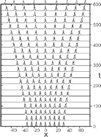
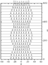
Figure 1: Left panel: $9$-soliton train with initial parameters as in eq. (48) with $r_{0}=8$ in the absence of a potential goes into free asymptotic regime. Solid lines: direct numerical simulation of the NLS equation (5); dashed lines: $\xi_{k}(t)$ as predicted by the CTC equations (50)-(53) with $V_{0}=V_{1}=V_{2}=0$ and $r_{0}=8$. Right panel: Evolution of a $9$-soliton train with the same initial parameters in the quadratic potential $V(x)=V_{2}x^{2}$ with $V_{2}=0.00005$. Solid lines: direct numerical simulation of the NLS equation (5); dashed lines: solution of the PCTC equations (50)-(53). Initially the train is placed symmetrically relative to the minimum of the potential at $x=0$.

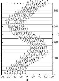
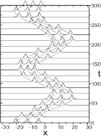
Figure 2: Harmonic oscillations of a N-soliton train initially shifted relative to the minimum of the quadratic potential $V(x)=V_{2}x^{2}$. Left panel: 9-soliton train, $V_{2}=0.00005$. Right panel: 3-soliton train, $V_{2}=0.001$. The IC of the both trains is given by (48) with $r_{0}=8$. In both panels solid lines correspond to direct simulations of the NLS equation (5), and dashed lines to numerical solution of the PCTC equations (50) - (53).

Figures 1 and 2 show good agreement between the PCTC model and the numerical solution of the perturbed NLS equation (5). They also show two types of effects of the quadratic potential on the motion of the $N$-soliton train: (i) the train performs contracting and expanding oscillations if its center of mass coincides with the minimum of the potential, (ii) the train oscillates around the minimum of the potential as a whole if its center of mass is shifted. In the last case contracting and expanding motions of the soliton train is superimposed to the center of mass dynamics. As one can see from the figures the period of this motion matches very well the one predicted by formula (III.1). Indeed, from eq. (III.1) it follows that the period of the center of mass motion is $T=2\pi/\sqrt{2V_{2}}$. For the parameters in fig. 2 we have $T\simeq 628$ (for 9-soliton train), $T\simeq 140$ (for $3$-soliton train). Similar is the dynamics also for the $7$-soliton train on Fig. 3; for the parameters choosen there we have $T\simeq 314$, in good agreement with the numerical simulations.

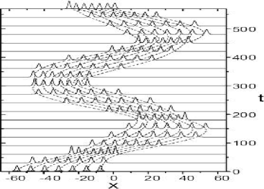
Figure 3: Dynamics of a 7-soliton train placed asymmetrically relative to the minimum of the trap $V(x)=0.0002x^{2}$. Solid lines: results of direct numerical simulations of the NLS equation (5). Dashed lines: result of solution of the PCTC system (50) - (53) for the center of mass $\xi_{i}$. The parameters of solitons are the same as in (48) with $r_{0}=8$. The initial shift of the soliton train relative to the minimum of the parabolic trap is $10\pi$.

The direct simulations of the NLS equation (5) shows that stronger parabolic trap may cause merging of individual solitons at times of contraction, and restoring of the original configuration when the train is expanded. This behavior reminds the phenomenon of ”missing solitons” observed in the experiment strecker . However, this situation is beyond the validity of the PCTC approach.

IV.2 Tilted periodic potential

Now we consider the dynamics of a N - soliton train in a tilted periodic potential, which is the combination of periodic and linear potentials

$$V(x)=A\cos(\Omega x+\Omega_{0})+Bx.$$ (56)

This potential is of particular interest in studies of Bose-Einstein condensates. A train of repulsive BEC loaded in such a potential (where the periodic potential was a 1D optical lattice and the linear one was due to the gravitation) exhibited Bloch oscillations anderson . At each period of these oscillations condensate atoms residing in individual optical lattice cells coherently tunneled through the potential barriers. This was the first experimental demonstration of a pulsed atomic laser anderson . Recently a new model of a pulsed atomic laser was theoretically developed in carr , where the solitons of attractive BEC were considered as carriers of coherent atomic pulses.

Controlled manipulation with matter - wave solitons is important issue in these applications. Below we demonstrate that solitons of attractive BEC confined in optical lattice can be flexible manipulated by adjustment of the strength of the linear potential. In Fig. 4 we show the extraction of different number of solitons from the 5-soliton train by increasing the strength of the linear potential $B$, as obtained from direct simulations of the NLS equation (1) and numerical integration of the PCTC system (38) - (41) with

$$M_{k}^{(2)} = {\pi A\Omega^{2}\over 8\nu_{k}}{1\over\sinh Z_{k}}\sin(\Omega\xi_{k}+\Omega_{0})-\frac{1}{2}B,$$ (57)

$$D_{k}^{(2)} = -{\pi^{2}A\Omega^{2}\over 16\nu_{k}^{2}}{\cosh Z_{k}\over\sinh^{2}Z_{k}}\cos(\Omega\xi_{k}+\Omega_{0})$$ (58)

$$- B\xi_{k}.$$

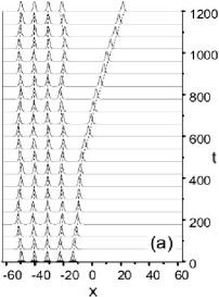
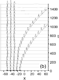
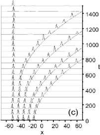
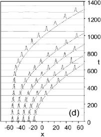
Figure 4: Controlled withdrawal of solitons from the 5-soliton train by adjusting the strength of the linear potential (56) with parameters: $A=-0.0005$, $\Omega=2\pi/9$, $\Omega_{0}=0$. Depending on the tilt, different number of solitons can be pulled out of the train: (a) one soliton at $B=-0.00003$, (b) two at $B=-0.00011$, (c) four at $B=-0.0002$ and (d) five at $B=-0.0003$. The initial phase difference and separation between neighboring solitons in the train are, respectively, $\pi$ and $9$. Initially the train is shifted by $-10\pi$ with respect to $x=0$ for graphical convenience. Solid and dashed lines correspond, respectively, to direct simulations of the NLS equation (5) and numerical integration of the PCTC system (59) - (62).

As is evident from Fig. 4, the PCTC model provides adequate description of the dynamics of a N-soliton train in a tilted periodic potential. A small divergence between predictions for the trajectory of the left border soliton in Fig. 4 (d), is due to the imperfect absorption of solitons from the right end of the integration domain. Reflected waves enter the integration domain and interact with solitons, which causes the discrepancy.

IV.3 Periodic potential

Another external potential in which the $N$-soliton train exhibits interesting dynamics is the periodic potential of the form $V(x)=A\cos(\Omega x+\Omega_{0})$. This case also may have a direct relevance to matter - wave soliton trains confined to optical lattices. The PCTC system in terms of soliton parameters has the form:

$${d\mu_{k}\over dt} = 16\nu_{0}^{3}\left(e^{-2\nu_{0}(\xi_{k+1}-\xi_{k})}\cos\Phi_{k}\right.$$ (59)

$$- \left.e^{-2\nu_{0}(\xi_{k}-\xi_{k-1})}\cos\Phi_{k-1}\right)+M_{k}^{(2)}(\nu_{k}),$$

$${d\nu_{k}\over dt} = 16\nu_{0}^{3}\left(e^{-2\nu_{0}(\xi_{k+1}-\xi_{k})}\sin\Phi_{k}\right.$$ (60)

$$\qquad-\left.e^{-2\nu_{0}(\xi_{k}-\xi_{k-1})}\sin\Phi_{k-1}\right),$$

$${d\xi_{k}\over dt} = 2\mu_{k},$$ (61)

$${d\delta_{k}\over dt} = 2(\mu_{k}^{2}+\nu_{k}^{2})+D_{k}^{(2)}(\nu_{k}),$$ (62)

where $M_{k}^{(2)}(\nu_{k})$, $D_{k}^{(2)}(\nu_{k})$ are given in (34) and (36), and $\Phi_{k}$ – in eq. (54).

Each soliton of the train experience confining force of the periodic potential and repulsive force of neighboring solitons. Therefore, equilibrium positions of solitons do not coincide with the minima of the periodic potential. Solitons placed initially at minima of the periodic potential (Fig. 5) perform small amplitude oscillations around these minima, provided that the strength of the potential is big enough to keep solitons confined. As opposed, the weak periodic potential is unable to confine solitons, and repulsive forces between neighboring solitons (at phase difference $\pi$) induces unbounded expansion of the train.

Figure 5: Solitons (continuous line) remain confined around the minima of the periodic potential $V(x)=A\cos(x)$ (dashed line) performing small amplitude oscillations if its strength is big enough $A=-0.1$.

In the intermediate region, when the confining force of the periodic potential is comparable with the repulsive forces of neighboring solitons, interesting dynamics can be observed such as the expulsion of bordering solitons from the train, as shown in the left panel of Fig. 6.

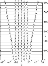
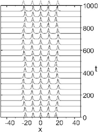
Figure 6: Left panel: The expulsion of solitons from the train, as obtained from direct simulations of the NLS equation (5) (solid lines), and as predicted by PCTC system (59)-(62) for the center of mass $\xi_{i}$ (dashed lines). The IC of the $7$-soliton train are given by (48) with $r_{0}=8$; the parameters of the periodic potential $V(x)=A\cos(\Omega x+\Omega_{0})$ are $A=-0.001,\ \Omega=\pi/4,\ \Omega_{0}=0$. Right panel: Oscillations of the 5-soliton train with IC given by (48) with $r_{0}=9$; in a moderately weak periodic potential, $A=-0.0005$, $\Omega=2\pi/9$, $\Omega_{0}=0$. Solid and dashed lines correspond, respectively, to numerical solution of the NLS eq. (5) and PCTC system (59) - (62).

This phenomenon, revealing the complexity of the internal dynamics of the train, can be explained as follows. Each soliton performs nonlinear oscillations within individual potential wells under repulsive forces from neighboring solitons. When the amplitude of oscillations of particular solitons grow and two solitons closely approach each other, a strong recoil momentum can cause the soliton to leave the train, overcoming barriers of the periodic potential. In Fig. 6 this happens with bordering solitons (the other solitons remain bounded under long time evolution). It is noteworthy to stress that this phenomenon is well described by the PCTC model, as is evident from Fig. 6, left panel.

On the right panel of the same figure we have similar IC as in (48) and we have choosen again the initial positions of the solitons to coincide with the minima of the periodic potential $V(x)=A\cos(\Omega x+\Omega_{0})$; i.e. $r_{0}=2\pi/\Omega$. The values of $A=-0.0005$ and $r_{0}=9$ in the right panel of Fig. 6 now are such that the solitons form a bound state. Therefore for any given initial distance $r_{0}$ there is a critical value $A_{\rm cr}(r_{0})$ for $A$ such that for $A>A_{\rm cr}(r_{0})$ the soliton train with IC (48) will form a bound state.

In contrast to the quadratic potentials, the weak periodic potential is unable to confine solitons, and repulsive forces between neighboring solitons (at $\nu_{k}(0)=1/2,\ \delta_{k}(0)=k\pi$) induces unbounded expansion of the train similar to what was shown in the left panel of Fig. 1.

The periodic potential can play stabilizing role also for the IC (49), when the zero phase difference between neighboring solitons correspond to their mutual attraction. If the periodic potential is strong enough, solitons do not experience collision. The weak periodic potential cannot prevent solitons from collisions, which eventually leads to destruction of the soliton train, as illustrated in Fig. 7. Again for any given initial distance $r_{0}$ there will be a critical value $A_{\rm cr}^{\prime}(r_{0})$ for $A$ such that for $A>A^{\prime}_{\rm cr}(r_{0})$ the soliton train with IC (49) will form a bound state avoiding collisions.

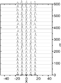
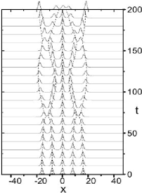
Figure 7: Dynamics of a 5-soliton train with zero phase difference between neighboring solitons, in the periodic potential $V(x)=A\cos(\Omega x+\Omega_{0})$ with $\Omega=\pi/4$, $\Omega_{0}=0$, and $r_{0}=8$. Left panel: When the periodic potential is strong enough $A=-0.02$, the N-soliton train remain confined, each soliton performing small amplitude oscillations around the minima of individual cells. Right panel: Weaker periodic potential $A=-0.01$ cannot prevent solitons from collisions, which destroy the train. Solid and dashed lines correspond, respectively, to numerical solution of the NLS eq. (5) and PCTC system (59) - (62).

Attractive interactions at zero phase difference between neighboring solitons can be balanced by expulsive force on solitons, if the train is positioned on an inverted parabolic trap. In this case solitons far from the center experience stronger expulsive force and leave the train, as illustrated in Fig. 8.

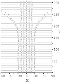
Figure 8: Stabilization of a soliton train in a combined potential (periodic $+$ inverted parabola): $V(x)=-0.02\cos(\Omega x)-0.000145x^{2}$. Separation between in-phase ($\delta_{k}=0$) solitons is $r_{0}=9$, $\Omega=2\pi/9$. Bordering solitons leave the train as they experience stronger expulsion, while the central ones remain bounded.

V Hamiltonian approach to perturbed NLS and CTC

The Hamiltonian method has played important role in the analysis of integrable and close to integrable nonlinear evolution equations and dynamical systems, see FaTa . In this section we will outline how this method can be used for the analysis of the $N$-soliton interactions.

The relation between the Hamiltonian properties of the NLS eq. and the CTC model was derived in VS-EPJ29 . Here we will show that this approach can be extended also to the perturbed versions of NLS and CTC. Indeed, the Hamiltonian of eq. (5) with $iR[u]=V(x)u(x,t)$ is equal to:

$$H = H_{\rm NLS}+H_{\rm V},$$ (63)

$$H_{\rm NLS} = \int_{-\infty}^{\infty}dx\,{1\over 2}\left(|u_{x}|^{2}-|u(x,t)|^{4}\right),$$ (64)

$$H_{\rm V} = \int_{-\infty}^{\infty}dx\,V(x)|u(x,t)|^{2},$$ (65)

One of the ways to derive the CTC from the NLS is based on the use of the variational method AndLis ; Arnold . Namely one constructs the Lagrangian of NLS, then takes an anzatz of the form:

$$u(x,t)=\sum_{k=1}^{N}u_{k}^{(\rm 1s)}(x,t),$$ (66)

and integrate over $x$ neglecting terms of order $\epsilon^{k}$ with $k>1$. Here $u_{k}^{(\rm 1s)}(x,t)$ is the one-soliton pulse with parameters $\mu_{k}$, $\nu_{k}$, $\xi_{k}$ and $\delta_{k}$. The results must depend only on the $4N$ soliton parameters. It was pointed out in VS-EPJ29 that if we apply this method directly to the Hamiltonian $H_{\rm NLS}$ we get additional singular in $\epsilon$ elements which are taken care of by a proper regularization. The regularized Hamiltonian is

$$H_{\rm reg} = 4(\mu_{0}^{2}+\nu_{0}^{2})C_{1}-4\mu_{0}C_{2}+H_{\rm NLS},$$ (67)

$$C_{1} = \int_{-\infty}^{\infty}dx\,|u(x,t)|^{2},$$

$$C_{2} = \int_{-\infty}^{\infty}dx\,{i\over 2}(u^{*}_{x}u(x,t)-u^{*}(x,t)u_{x}),$$

Then one can show that

$$H_{\rm reg}=32\nu_{0}H_{\rm CTC}+\mathrm{const\,}$$ (68)

where $H_{\rm CTC}$ is the Hamiltonian of the CTC. It is obtained from the Toda chain Hamiltonian:

$$H_{\rm TC}=\sum_{k=1}^{N}{1\over 2}p_{k}^{2}+\sum_{k=1}^{N-1}e^{q_{k+1}-q_{k}},$$ (69)

by a complexification procedure after which the dynamical variables become complex-valued:

$$p_{k}\to P_{k}=p_{0,k}+ip_{1,k},\qquad q_{k}\to Q_{k}=q_{0,k}+iq_{1,k},$$ (70)

which must satisfy the Poisson brackets:

$$\{p_{0,k},q_{0,s}\}=\delta_{ks},\qquad\{p_{1,k},q_{1,s}\}=-\delta_{ks},$$ (71)

$$\{p_{0,k},q_{1,s}\}=0,\qquad\{p_{1,k},q_{0,s}\}=0,$$ (72)

Then the CTC can be written down as a standard Hamiltonian system with $2N$-degrees of freedom and Hamiltonian provided by the real part of the complexified $H_{\rm TC}$:

$$H_{\rm CTC} = \sum_{k=1}^{N}{1\over 2}(p_{0,k}^{2}-p_{1,k}^{2})$$ (73)

$$+ 16\nu_{0}^{2}\sum_{k=1}^{N-1}e^{q_{0,k+1}-q_{0,k}}\cos(q_{1,k+1}-q_{1,k}),$$

$$p_{0,k}={dq_{0,k}\over dt}=-4\nu_{0}\mu_{k},\qquad p_{1,k}={dq_{1,k}\over dt}=-4\nu_{0}\nu_{k}.$$ (74)

It remains to replace $q_{0,k}$ and $q_{1,k}$ in terms of the soliton parameters in order to get the final expression for $H_{\rm CTC}$.

Let us now derive the Hamiltonian for the perturbed CTC. To this end we will evaluate $H_{\rm V}$ in terms of the soliton parameters. Inserting the anzats (66) into the integrand for $H_{\rm V}$ we obtain two types of terms. The first type is

$$H_{\rm V} = \sum_{k=1}^{N}H_{k}+\sum_{k=1}^{N}(H_{k,k-1}+H_{k,k+1}),$$ (75)

$$H_{k} = \int_{-\infty}^{\infty}dx\,V(x)|u_{k}^{(\rm 1s)}(x,t)|^{2},$$ (76)

$$H_{k,k-1} = \int_{-\infty}^{\infty}dx\,V(x)(u_{k}^{(\rm 1s),*}u_{k-1}^{(\rm 1s)})(x,t).$$

In what follows we will neglect the terms $H_{k,k-1}$ as compared to $H_{k}$, because their ratio is of the order of $\epsilon$. The integrals in (76) for the quadratic and periodic potentials have the form:

$$H_{k} = 4\nu_{k}\left(\left(V_{2}(\xi_{k}^{2}-{\pi^{2}\over 48\nu_{k}^{2}}\right)+V_{1}\xi_{k}+V_{0}\right)$$ (77)

$$+ {\pi A\Omega\over\sinh Z_{k}}\cos(\Omega\xi_{k}+\Omega_{0}).$$

One can also evaluate the Poisson brackets between the soliton parameters inserting the expressions for $p_{\alpha,k}$ and $q_{\beta,s}$ with $\alpha,\beta=0,1$ into (71). We skip the lengthy calculations here and only note that these Poisson brackets combined with the Hamiltonian

$$H_{\rm PCTC} = H_{\rm CTC}+\sum_{k=1}^{N}H_{k}$$ (78)

$$= H_{\rm CM}+H_{\rm V},$$ (79)

indeed produce the equations of motion for the PCTC.

Our next step is to separate the center of mass motion described by $H_{\rm CM}$:

$$H_{\rm CM} = N\left(8\nu_{0}^{2}(\mu_{0}^{2}-\nu_{0}^{2})+4\nu_{0}(V_{2}\xi_{0}^{2}+V_{1}\xi_{0}+V_{0})\right.$$ (80)

$$- \left.{\pi A\Omega\over\sinh({\pi\Omega\over 4\nu_{0}})}\cos(\Omega\xi_{0}+\Omega_{0})\right),$$

where the subscript 0 stands for the average value of the corresponding parameter, e.g. $\xi_{0}=1/N\sum_{k=1}^{N}\xi_{k}$. Then the Hamiltonian $H_{\rm V}$ would describe the relative motion of the solitons. We will express it as a function of the averaged parameters $\mu_{0}$, …, $\delta_{0}$ and the relative parameters:

$$\widetilde{\mu}_{k}=\mu_{k}-\mu_{0},\qquad\widetilde{\nu}_{k}=\nu_{k}-\nu_{0},$$

$$\widetilde{\xi}_{k}=\xi_{k}-\xi_{0},\qquad\widetilde{\delta}=\delta_{k}-\delta_{0},$$ (81)

Note, that only $N-1$ of the relative parameters are independent; obviously they satisfy $\sum_{k=1}^{N}\widetilde{X}_{k}=0$ where $\widetilde{X}_{k}$ stands for $\widetilde{\mu}_{k}$, …, $\widetilde{\delta}_{k}$.

In evaluating $H_{\rm V}$ we will neglect higher order terms, i.e. terms of the order $\epsilon^{3/2}$ and higher, as well as terms of the order $V_{s}\epsilon^{1/2}$, $A\epsilon^{1/2}$ and higher. As a result $H_{\rm CM}$ and $H_{\rm V}$ simplify to:

$$H_{\rm CM} = 8\nu_{0}^{2}(\mu_{0}^{2}-\nu_{0}^{2})+4\nu_{0}\left(V_{2}\xi_{0}^{2}+V_{1}\xi_{0}+V_{0}-{V_{2}\pi^{2}\over 48\nu_{0}^{2}}\right)$$ (82)

$$+ {\pi A\Omega\over\sinh Z_{0}}\cos(\Omega\xi_{0}+\Omega_{0}),$$

$$H_{\rm V} = 8\nu_{0}^{2}\sum_{k=1}^{N}(\widetilde{\mu}_{k}^{2}-\widetilde{\nu}_{k}^{2}+\widetilde{H}_{k})$$ (83)

$$+ 16\nu_{0}^{2}\sum_{k=1}^{N-1}e^{q_{0,k+1}-q_{0,k}}\cos(q_{1,k+1}-q_{1,k}),$$

$$\widetilde{H}_{k} = 4\nu_{0}V_{2}(\xi_{k}-\xi_{0})^{2}$$ (84)

$$+ {\pi A\Omega\over\sinh Z_{0}}(\cos(\Omega\xi_{k}+\Omega_{0})-\cos(\Omega\xi_{0}+\Omega_{0})).$$

The Hamiltonian $H_{\rm CM}$ which describes the center of mass motion is more simple than $H_{\rm V}$ and often one is able to solve explicitly the corresponding equations of motion, see Section IV. The next step would be, using the known expressions for the averaged variables $\mu_{0}(t)$, …, $\delta_{0}(t)$ to insert them into $H_{\rm V}$ and try to analyze the corresponding equations of motion. This would provide us with information about the relative motion of the solitons around the center of mass. Usually we get a set of nonlinear and non-integrable ODE.

Our idea here is to use the explicit form of $H_{\rm V}$ for the estimation of the critical values of potential strengths $A$, $V_{2}$, $V_{1}$ for which the soliton motion becomes qualitatively different. Doing this we are making use of the following hypothesis based on the well known fact that bound states have negative energies while asymptotically free motions should correspond to positive energies. Therefore we evaluate the Hamiltonian $H_{\rm V}$ inserting in it the initial soliton parameters along with the known expressions for $\mu_{0}$, …, $\delta_{0}$. If the result is negative we may expect that the relative motion of the solitons will be bounded; otherwise one may expect that at least one (or more) of the solitons will move away from the others. The critical value of the corresponding constants will be derived below with the condition $H_{\rm V}=0$.

Assume we have only periodic potential present and the initial soliton configuration is (48). For $A=0$ the solitons will go into asymptotically free regime. Switching on the self-consistent periodic potentials (such that the solitons initially are located at its minima) it is natural to expect that for $A>A_{\rm cr}$ the solitons will be stabilized into a bound state. Then from the condition $H_{\rm V}=0$ we get:

$$A_{\rm cr}=-\left(1-{1\over N}\right){64\nu_{0}^{4}\over\pi\Omega}e^{-2\nu_{0}r_{0}}\sinh{\pi\Omega\over 4\nu_{0}}.$$ (85)

Note that the critical values generically should depend not only on the number of solitons $N$, but also on the initial configuration. The approach we used is not very sensitive to this. It can not provide us with the intermediary critical values when the soliton train is stabilized after emmiting two or more solitons.

We compared the theoretical predictions for $A_{\rm cr}$ from eq. (85) with the data coming from the numeric solutions of the corresponding PCTC for different choices of the initial distance between the solitons $r_{0}$. The results are collected into the table 1. The conclusion is that eq. (85) provides correct dependence of $A_{\rm cr}$ on $r_{0}$ up to an overall constant factor of the order of $1.5$.

$r_{0}$	$A_{\rm cr}^{\rm exp}$	$A_{\rm cr}^{\rm th}$	$A_{\rm cr}^{\rm exp}/A_{\rm cr}^{\rm th}$
$2\pi$	-0.0053	-0.00365	1.45
7	-0.0025	-0.00166	1.51
8	-0.00084	-0.00057	1.47
9	-0.00030	-0.00020	1.50

Table 1: The values of $A_{\rm cr}^{\rm exp}$ obtained from numeric simulations with PCTC versus $A_{\rm cr}^{\rm th}$ obtained from eq. (85) for $N=3$.

In the next table 2 we summarize two sets of critical values for the $5$-soliton trains. From our numeric experiment we derive two critical values of $A$. The first one $A_{\rm cr}^{\rm 5,exp}$ describes the value of $A$ above which all $5$ solitons form a bound state; the second one $A_{\rm cr}^{\rm 3,exp}$ shows the value of $A$ above which the three middle solitons form a bound state while the two end ones separate.

$r_{0}$	$A_{\rm cr}^{\rm 5,exp}$	$A_{\rm cr}^{\rm 3,exp}$	$A_{\rm cr}^{\rm th}$	$A_{\rm 5,cr}^{\rm exp}/A_{\rm cr}^{\rm th}$	$A_{\rm 3,cr}^{\rm exp}/A_{\rm cr}^{\rm th}$
$2\pi$	-0.0068	-0.0029	-0.0044	1.55	0.66
7	-0.0031	-0.0013	-0.0020	1.56	0.65
8	-0.00115	-0.00043	-0.00068	1.68	0.63
9	-0.00041	-0.000155	- 0.00024	1.71	0.65

Table 2: The values of $A_{\rm cr}^{\rm 5,exp}$ and $A_{\rm cr}^{\rm 3,exp}$ obtained from numeric simulations with PCTC versus $A_{\rm cr}^{\rm th}$ obtained from eq. (85) for $N=5$.

Again we see, that formula (85) describes correctly the dependence of both critical values on $r_{0}$.

VI Conclusions

We have studied the dynamics of a $N$-soliton train confined to external fields (quadratic, periodic and tilted potentials). Both the analytical treatment in the framework of the PCTC model, and numerical analysis by direct simulations of the underlying NLS equation show that the PCTC is adequate for description of the adiabatic $N$-soliton interactions in weak external potentials. Hamiltonian approach for the perturbed NLS and CTC has been developed, and applied to the analysis of the soliton ”expulsion” from the train, which is confined to a periodic potential.

As a physical system of direct relevance we have considered matter-wave soliton trains in magnetic traps and optical lattices. In the range of parameters for the trapping potential, used in the BEC soliton train experiments, we found a good agreement between the analytical estimates based on the PCTC model and numerical simulations of the governing NLS equation. In what concerns the critical strength of the periodic potential at which the soliton expulsion occurs, analytical predictions qualitatively agree with numerical simulations. The developed theory can be useful for controlled manipulation with matter-wave soliton trains.

References

• (1) A. Hasegawa and Y. Kodama, Solitons in optical communications, (Oxford, Clarendon Press, 1995).
• (2) Y. Kivshar and G. Agrawal, Optical Solitons: From Fibers to Photonic Crystals, (Academic Press, San Diego, 2003).
• (3) A. Barone, G. Paternó, Physics and Applications of the Josephson Effect, N.Y., Wiley, (1982).
• (4) F. Kh. Abdullaev, A. Gammal, A. M. Kamchatnov and L. Tomio, Int. J. Mod. Phys. B 19, 3415 (2005); V. A. Brazhnyi and V. V. Konotop, Mod. Phys. Lett. B 18, 267 (2004).
• (5) For recent progress in theory and applications of BEC see the special issue: J. Phys. B. vol.38, No.9 (2005).
• (6) K. E. Strecker, G. B. Partridge, A. G. Truscott, and R. G. Hulet, Nature, 417, 150 (2002); K. E. Strecker et al., Advances in Space Research 35, 78 (2005).
• (7) L. Khaykovich, F. Schreck, G. Ferrari, T. Bourdel, J. Cubizolles, L. D. Carr, Y. Castin, and C. Salomon, Science 296, 1290 (2002).
• (8) V. I. Karpman, V. V. Solov’ev, Physica D 3D, 487-502, (1981).
• (9) V. S. Gerdjikov, D. J. Kaup, I. M. Uzunov, E. G. Evstatiev, Phys. Rev. Lett. 77, 3943-3946 (1996).
• (10) V. S. Gerdjikov, I. M. Uzunov, E. G. Evstatiev, G. L. Diankov, Phys. Rev. E 55, No 5, 6039-6060 (1997).
• (11) J. M. Arnold, JOSA A 15, 1450-1458 (1998); Phys. Rev. E 60, 979-986 (1999).
• (12) V. S. Gerdjikov, E. G. Evstatiev, D. J. Kaup, G. L. Diankov, I. M. Uzunov, Phys. Lett. A 241, 323-328 (1998).
• (13) V. S. Gerdjikov, On Modelling Adiabatic $N$-soliton Interactions. Effects of perturbations. In ”Nonlinear Waves: Classical and Quantum Aspects”, Eds.: F. Kh. Abdullaev and V. Konotop. (Kluwer, 2004), 15 - 28.
• (14) E. V. Doktorov, N. P. Matsuka, V. M. Rothos. Phys. Rev. E 69, 056607 (2004).
• (15) Y. Kodama, A. Hasegawa, IEEE J. of Quant. Electron. QE-23, 510 - 524 (1987).
• (16) V. S. Gerdjikov, M. I. Ivanov, P. P. Kulish, Theor. Math. Phys. 44, No.3, 342–357, (1980), (In Russian). V. S. Gerdjikov, M. I. Ivanov, Bulgarian J. Phys. 10, No.1, 13–26; No.2, 130–143, (1983), (In Russian).
• (17) V. S. Shchesnovich and E. V. Doktorov, Physica D 129, 115 (1999); E. V. Doktorov and V. S. Shchesnovich, J. Math. Phys. 36, 7009 (1995).
• (18) V. S. Gerdjikov, E. V. Doktorov, J. Yang, Phys. Rev. E 64, 056617 (2001).
• (19) V. S. Gerdjikov, I. M. Uzunov, Physica D 152-153, 355-362 (2001).
• (20) V. E. Zakharov, S. V. Manakov, S. P. Novikov, L. P. Pitaevskii, Theory of solitons: the inverse scattering method. (Plenum, N.Y.: Consultants Bureau, 1984).
• (21) L. A. Takhtadjan and L. D.  Fadeev, Hamiltonian Approach to Soliton Theory  (Springer Verlag, Berlin, 1986).
• (22) S. V. Manakov, JETPh 67, 543 (1974); H. Flaschka. Phys. Rev. B9, 1924–1925, (1974);
• (23) V. S. Gerdjikov, Complex Toda Chain – an Integrable Universal Model for Adiabatic $N$-soliton Interactions. In Proc. of the Workshop ”Nonlinear Physics: Theory and Experiment. II”, Gallipoli, June-July 2002; Eds.: M. Ablowitz, M. Boiti, F. Pempinelli, B. Prinari. p. 64-70 (2003).
• (24) J. C. Bronski, L. D. Carr, B. Deconinck, J. N. Kutz, Phys. Rev. E 63, 036612 (2001); Phys. Rev. Lett. 86, 1402–1405 (2001); J. C. Bronski, L. D. Carr, R. Carretero-Gonzales, B. Deconinck, J. N. Kutz, K. Promislow, Phys. Rev. E 64, 056615 (2001); F. Kh. Abdullaev, B. B. Baizakov, S. A. Darmanyan, V. V. Konotop, M. Salerno, Phys. Rev. A 64, 043606 (2001).
• (25) R. Carretero-Gonzalez and K. Promislow, Phys. Rev. A 66, 033610 (2002).
• (26) V. S. Gerdjikov, B. B. Baizakov, M. Salerno, Modelling adiabatic N-soliton interactions and perturbations. In: Proceedings of the workshop ”Nonlinear Physics: Theory and Experiment. III”, Gallipoli, 2004;
Eds.: M. Ablowitz, M. Boiti, F. Pempinelli, B. Prinari, Theor. Math. Phys. 144, No. 2, 1138–1146 (2005) .
V. S. Gerdjikov, B. B. Baizakov, On Modelling Adiabatic $N$-soliton Interactions and Perturbations. Effects of external potentials. Report at the International Conference ”Gravity, astrophysics and strings at the Black sea”, Kiten, Bulgaria, June 10 - 16 (2004).
• (27) S. Wabnitz. Electron. Lett. 29, 1711 (1993);
• (28) I. M. Uzunov, M. Gölles, F. Lederer, JOSA B 12, No. 6, 1164 (1995);
I. M. Uzunov, M. Gölles, F. Lederer, Phys. Rev. E 52, 1059-1071 (1995).
• (29) J. Moser, In Dynamical Systems, Theory and Applications. Lecture Notes in Physics, v. 38, Springer Verlag, (1975), p. 467.
• (30) V. S. Gerdjikov, E. G. Evstatiev, R. I. Ivanov, The complex Toda chains and the simple Lie algebras – solutions and large time asymptotics, J. Phys. A: Math & Gen. 31, 8221-8232 (1998).
• (31) T. R. Taha and M. J. Ablowitz, J. Comp. Phys. 55, 203 (1984).
• (32) W. H. Press, S. A. Teukolsky, W. T. Vetterling, and B. P. Flannery, Numerical Recipes. The Art of Scientific Computing. (Cambridge University Press, 1996).
• (33) B. P. Anderson, M. A. Kasevich, Science, 282, 1686 (1998).
• (34) L. D. Carr and J. Brand, Phys. Rev. A 70, 033607 (2004).
• (35) V. S. Gerdjikov. European J. Phys. 29B, 237-242 (2002).
• (36) D. Anderson, and M. Lisak, Opt. Lett. 11, 174 (1986).