Spin Nematic Phase in $S$=1 Triangular Antiferromagnets

Abstract

Spin nematic order is investigated for a $S$=1 spin model on triangular lattice with bilinear-biquadratic interactions. We particularly studied an antiferro nematic order phase with three-sublattice structure, and magnetic properties are calculated at zero temperature by means of bosonization. Two types of bosonic excitations are found. One is a gapless excitation with linear energy dispersion around $\mathbf{k}\sim\mathbf{0}$, and this leads to a finite spin susceptibility at $T=0$ and would have a specific heat $C(T)\sim T^{2}$ at low temperatures. These behaviors can explain many of characteristic features of recently discovered spin liquid state in the triangular magnet, NiGa₂S₄.

The concept of spin liquid was introduced thirty years ago by P. W. Anderson anderson , as a quantum critical state in which the spin-spin correlation function does not show a real long-range order but a power-law behavior. This issue has been studied intensively since then both theoretically and experimentally. Frustration and quantum fluctuations are considered two ingredients to realize a spin liquid, and a spin-1/2 Heisenberg antiferromagnet on triangular lattice was the first candidate. Many antiferromagnetic materials with triangular lattice structure have been studied to see if they may show a spin liquid behavior, but most of them turned out to exhibit some long-range order at low temperatures. Very few exceptions are ${}^{3}\mathrm{He}$ thin layer He and organic $\kappa$-(BEDT-TTF)₂Cu₂(CN)₃ BEDT , and just recently a new spin-liquid material NiGa₂S₄ was discovered nigas . While the former two are spin-1/2 system, NiGa₂S₄ is a spin-1 system.

In NiGa₂S₄, spins of Ni²⁺ ions form triangular layers with undistorted regular triangle units, and the layers are stacked along the c-axis. These layers are effectively decoupled, since the Ni-Ni distance is more than three times longer between layers. This system showed various low-temperature properties that indicate a spin liquid state. First of all, no singularity was observed in specific heat down to the lowest temperature, $T$=0.3 K, meaning the absence of phase transitions. Moreover, the specific heat shows a power-law behavior, $C\sim T^{2}$, below 10K. Secondly, the magnetic susceptibility gradually increased with decreasing temperature, and approached a finite value. Thirdly, neutron experiment observed a peak at an incommensurate wavevector $\mathbf{Q}$$\sim$$(\frac{\pi}{\sqrt{3}},0)$. However, this was not a magnetic Bragg peak, and spin correlation length did not diverge but saturated to about $\xi$$\sim$ 20Å, only seven lattice units.

Absence of magnetic long-range order and presence of critical behaviors are necessary conditions to identify a spin liquid, and these were satisfied in NiGa₂S₄. These may suggest a finite spin gap instead, but this contradicts a nonvanishing temperature dependence of susceptibility. In this paper, we will examine the possibility of a hidden order that reproduce similar low-temperature properties as critical spin liquid states.

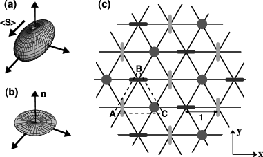
Figure 1: Spin quadrupole moment $\mathcal{Q}_{\mu\mu^{\prime}}$ of a single-site wavefunction when (a) $\langle\mathbf{S}\rangle\neq\mathbf{0}$ and (b) $\langle\mathbf{S}\rangle=\mathbf{0}$. (c) Three-sublattice nematic order. Dotted triangle shows a unit cell of the ordered state.

Possible order parameters are not ordinary static spin dipole moments $\langle\mathbf{S}\rangle$, since neutron experiment did not observe magnetic Bragg peaks. We should note that Ni²⁺ ions do not have orbital degrees of freedom nigas , and that we can describe this system as a pure spin model with no spin anisotropy. Therefore, if any long-range order exists, its order parameter should be represented in terms of spin operators. We will investigate the simplest candidate, spin quadrupole moments, $Q_{\mu\mu^{\prime}}=\frac{1}{2}\langle S^{\mu}S^{\mu^{\prime}}+S^{\mu^{\prime}}S^{\mu}\rangle-\frac{1}{3}S(S+1)\delta_{\mu\mu^{\prime}}$, where $\mu$ is spin index, and this also corresponds to nematic order nematic ; matveev . The nematic order parameter $Q_{\mu\nu}$ describes anisotropy of spin fluctuations, not static moment, and can be nonzero only if $S\geq 1$ momoi . In NiGa₂S₄, local spins are $S$=1 and therefore we consider the nematic order parameter defined at each site. Neutron experiment found a peak of scattering at incommensurate wavevectors $\mathbf{Q}$, not at $\mathbf{q}$=$\mathbf{0}$ or Brillouin zone boundary. This suggests that the expected nematic order is not uniform but modulates in space, i.e., some antiferro order.

To describe this order, the standard Heisenberg Hamiltonian is not sufficient, since it is believed to have a 120-degree magnetic long range order bernu . We use a spin-1 model with additional biquadratic interactions between nearest neighbor sites on the triangular lattice,

$$H=\sum_{\langle i,j\rangle}\left[J\mathbf{S}_{i}\cdot\mathbf{S}_{j}+K(\mathbf{S}_{i}\cdot\mathbf{S}_{j})^{2}\right].$$ (1)

This model has been studied by mean field analysis and numerical calculations nematic_papers . The mean field analysis at $T=0$ showed two nematic phases. One is the region of $K$$<$$J$$<$0 and a uniform nematic order appears. The other one is an antiferro nematic order and it is predicted in the region of 0$<$$J$$<$$K$. The latter is our expected case, and we will investigate that parameter region. We should note that the model (1) is a phenomenological Hamiltonian introduced to describe an expected modulated nematic order. While the antiferromagnetic bilinear terms are naturally expected from superexchange processes, the biquadratic terms are also present as higher-oder processes of virtual electron hopping, but usually it is expected that $|J|$$>$$|K|$. In our choice of model, it is assumed that both coupling constants are renormalized in the low-energy sector from their microscopic values such that 0$<$$J$$<$$K$, but this should be examined in future work.

We investigate the nature of nematic order parameter $Q_{\mu\nu}$ in more details for the $S$=1 case. To see this, it is more convenient not to subtract the constant term in the definition, and consider $\mathcal{Q}_{\mu\nu}(\mathbf{r})$=$\frac{1}{2}\langle S^{\mu}(\mathbf{r})S^{\nu}(\mathbf{r})$ +$S^{\nu}(\mathbf{r})S^{\mu}(\mathbf{r})\rangle$ at site $\mathbf{r}$. We introduce this tensor at each site $\mathbf{r}$ defined for a local wavefunction, and calculate its average by taking account of fluctuations in space and time. In the $S$=1 case, we can show that for any single-site wavefunctions, the three eigenvalues of $\mathcal{Q}_{\mu\nu}$ are $\lambda_{1,2}$=$\frac{1}{2}(1\mp\sqrt{1-\langle\mathbf{S}\rangle^{2}})$, and $\lambda_{3}$=1, and ${\mathcal{Q}}_{\mu\nu}$ is represented as an ellipsoid as shown in Fig. 1(a). Therefore, when $\langle\mathbf{S}\rangle$=$\mathbf{0}$, spin fluctuations are like disk and have zero amplitude in one direction in spin space (see Fig. 1(b)). This is characterized by the director vector $\mathbf{n}$ that is perpendicular to the disk. The corresponding wavefunction $|\psi_{\mathbf{n}}\rangle$ is the coherence state such that $(\mathbf{n}\cdot\mathbf{S})|\psi_{\mathbf{n}}\rangle$=0, namely rotated $|\mbox{$S_{z}$=0}\rangle$ state with quantization axis parallel to $\mathbf{n}$.

Mean field solution of the model (1) is easily obtained for the triangle lattice, and it is a three-sublattice nematic order shown in Fig. 1(c). The directors in the three sublattices are orthogonal to each other, and without generality, we can set $\mathbf{n}_{A}$$\parallel$$x$, $\mathbf{n}_{B}$$\parallel$$y$, and $\mathbf{n}_{C}$$\parallel$$z$, where $A$-$C$ are sublattice indices. Then the mean-field ground state is a direct product of local states $|\Psi_{\mathrm{MF}}\rangle$= $\prod_{\mathbf{R}}|\mbox{$S_{x}$=0}\rangle_{A,\mathbf{R}}$ $\otimes$ $|\mbox{$S_{y}$=0}\rangle_{B,\mathbf{R}}$ $\otimes$ $|\mbox{$S_{z}$=0}\rangle_{C,\mathbf{R}}$. Here, $\mathbf{r}$=$(j,\mathbf{R})$, with sublattice index $j\in\{A,B,C\}$ and unit-cell coordinate $\mathbf{R}$.

We now describe quantum fluctuations of the mean-field solution by introducing bosons. Each $S$=1 spin has three local states, and one of them corresponds to a mean-field solution. Following Matveev matveev , we consider it as a local vacuum and the other two excited states as one-boson states. To be specific, let us consider a site in the C-sublattice. $|\mbox{$S_{z}$=0}\rangle_{C,\mathbf{R}}$ is local vacuum $|\mbox{vac}\rangle_{C,\mathbf{R}}$, and the other states are represented as $|\mbox{$S_{z}$=$\pm$1}\rangle_{C,\mathbf{R}}$= $2^{-1/2}$ $(\alpha_{C,\mathbf{R}}^{\dagger}$$\pm$$i\beta_{C,\mathbf{R}}^{\dagger})$ $|\mbox{vac}\rangle_{C,\mathbf{R}}$, by boson creation operators $\alpha^{\dagger}$ and $\beta^{\dagger}$. Then spin operators are represented as $S_{C\mathbf{R}}^{x}$=$\alpha_{C\mathbf{R}}^{\dagger}$+$\alpha_{C\mathbf{R}}$, $S_{C\mathbf{R}}^{y}$=$\beta_{C\mathbf{R}}^{\dagger}$+$\beta_{C\mathbf{R}}$, $S_{C\mathbf{R}}^{z}$=$-i(\alpha_{C\mathbf{R}}^{\dagger}\beta_{C\mathbf{R}}$ $-$$\beta_{C\mathbf{R}}^{\dagger}\alpha_{C\mathbf{R}})$. In a similar way, two types of bosons are also introduced for the A- and B-sublattices. It is noted that these bosons are subject to constraint, $\alpha_{j\mathbf{R}}^{\dagger}\alpha_{j\mathbf{R}}$ +$\beta_{j\mathbf{R}}^{\dagger}\beta_{j\mathbf{R}}$$\leq$1, or equivalently $\alpha_{j\mathbf{R}}^{2}$=$\beta_{j\mathbf{R}}^{2}$ =$\alpha_{j\mathbf{R}}\beta_{j\mathbf{R}}$=0.

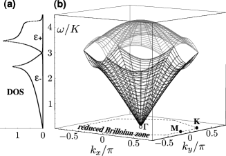
Figure 2: Two types of excitations for $J/K$=0.5.(a) Density of states with logarithmically divergent van Hove singularity. (b) Energy dispersion.

We replace spin operators in the model (1) by bosons and then neglect their interactions. This corresponds to Gaussian approximation of spin fluctuations. After taking the Fourier transformation, the obtained boson hamiltonian reads, $H_{b}$=$3K\Omega$+ $H(\beta_{A},\alpha_{B})$+ $H(\beta_{B},\alpha_{C})$+ $H(\beta_{C},\alpha_{A})$, and

$$H(\beta_{j},\alpha_{j^{\prime}})=3K\sum_{\mathbf{k}}\left(\beta_{j\mathbf{k}}^{\dagger}\beta_{j\mathbf{k}}+\alpha_{j^{\prime}\mathbf{k}}^{\dagger}\alpha_{j^{\prime}\mathbf{k}}\right)$$

$$+3\sum_{\mathbf{k}}\left\{\gamma_{\mathbf{k}}\left[(\mbox{$J$$-$$K$})\beta_{j\mathbf{k}}^{\dagger}\alpha_{j^{\prime}\mathbf{k}}+J\beta_{j\mathbf{k}}^{\dagger}\alpha_{j^{\prime}\mathbf{k}}^{\dagger}\right]+\mbox{h.c.}\right\},$$ (2)

where $\Omega$ is the number of unit cells and the sum is taken over the reduced Brillouin zone of the three-sublattice order, and $\gamma_{\mathbf{k}}$=$\frac{1}{3}e^{-ik_{x}}$+ $\frac{2}{3}e^{ik_{x}/2}\cos(\sqrt{3}k_{y}/2)$. Here we set the lattice constant being unity. Each type of bosons interact with only another one type of bosons, and therefore we can easily diagonalize the boson hamiltonian by Bogoliubov transformation, $H_{b}=\sum_{\mathbf{k},j\in\{A,B,C\}}\sum_{m=\pm}\varepsilon_{m,\mathbf{k}}b_{m\mathbf{k}}^{\dagger}b_{m\mathbf{k}}+E_{0}$ with the eigenenergy

$$\varepsilon_{\pm,\mathbf{k}}=3K\sqrt{(1\pm|\gamma_{\mathbf{k}}|)(1\pm\kappa|\gamma_{\mathbf{k}}|)},\quad\kappa=1-2J/K.$$ (3)

The dispersions and density of states are plotted in Fig. 2 for $J/K$=0.5. The $\varepsilon_{-}$ branch is gapless excitation with asymptotically linear dispersion, $\varepsilon_{-,\mathbf{k}}\sim 3\sqrt{JK/2}\,|\mathbf{k}|$ around $\mathbf{k}$=$\mathbf{0}$. The $\varepsilon_{+}$ branch is gapful excitation, and it touches the $\varepsilon_{-}$ branch at energy $3K$ on the six corners of the Brillouin zone. The $J=0$ case is special, since the mean-field state is an exact eigenstate, and the gapless excitations have a quadratic dispersion, $\varepsilon_{-,\mathbf{k}}\propto k^{2}$. The $J$=$K$ case is also special and the $\varepsilon_{+}$ branch becomes gapless and degenerate with the $\varepsilon_{-}$ branch.

These two branches describe bosonic elementary excitations in the nematic order, and in particular, the gapless branch is the Goldstone mode corresponding to the broken spin rotation symmetry goldstone . These elementary excitations contribute to magnetic fluctuations, and therefore, we may call them magnons also in this case. The Gaussian approximation is checked by calculating $\rho$= $\langle\alpha_{\mathbf{r}}^{\dagger}\alpha_{\mathbf{r}}+\beta_{\mathbf{r}}^{\dagger}\beta_{\mathbf{r}}\rangle$, the density of mean-field excited states. $\rho(J)$ increases from 0 at $J$=0 to about 0.15 at $J$=$K$, which was much smaller than 1, and the approximation is justified semi-quantitatively.

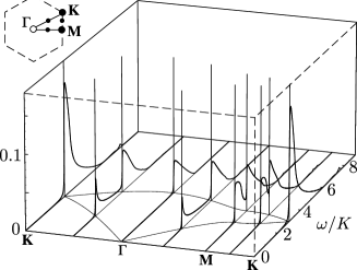
Figure 3: Dynamical spin structure factor $\sum_{j}S_{jj}^{\mu\mu}(\mathbf{k},\omega)$ for $J/K$=0.5. Dispersion of two magnon branches is also plotted.

The dynamical spin structure factor is given at zero temperature by $S^{\mu\mu^{\prime}}_{jj^{\prime}}(\mathbf{k},\omega)$= $\sum_{\nu}\langle 0|S^{\mu}_{j,-\mathbf{k}}|\nu\rangle$ $\langle\nu|S^{\mu^{\prime}}_{j^{\prime},\mathbf{k}}|0\rangle$ $\delta(\mbox{$\omega$$-$$E_{\nu}$+$E_{0}$})$, where $|\nu\rangle$ is the eigenstate with energy $E_{\nu}$ and $|0\rangle$ is the ground state. $S^{\mu}_{j,\mathbf{k}}$ is the Fourier transform of the spin on the $j$-sublattice. Structure factor $S^{\mu\mu^{\prime}}_{jj^{\prime}}(\mathbf{k},\omega)$ is diagonal with respect to spin indices $\mu$ and $\mu^{\prime}$. $\{S^{xx}_{jj^{\prime}}(\mathbf{k},\omega)\}$ is obtained as

$$\left[\begin{array}[]{ccc}S^{xx}_{AA}&S^{xx}_{AB}&S^{xx}_{AC}\\ S^{xx}_{BA}&S^{xx}_{BB}&S^{xx}_{BC}\\ S^{xx}_{CA}&S^{xx}_{CB}&S^{xx}_{CC}\end{array}\right]=\left[\begin{array}[]{ccc}F_{2}&0&0\\ 0&F_{1}^{(0)}&e^{-i\phi_{\mathbf{k}}}F_{1}^{(1)}\\ 0&e^{i\phi_{\mathbf{k}}}F_{1}^{(1)}&F_{1}^{(0)}\end{array}\right],$$ (4)

where $e^{i\phi_{\mathbf{k}}}=\gamma_{\mathbf{k}}/|\gamma_{\mathbf{k}}|$. $F_{1}^{(p)}(\mathbf{k},\omega)$ and $F_{2}(\mathbf{k},\omega)$ denote one and two-magnon contributions:

$$F_{1}^{(p)}(\mathbf{k},\omega) = \frac{1}{2}\sum_{m=\pm}(-m)^{p}e^{2\theta_{m,\mathbf{k}}}\delta(\omega-\varepsilon_{m,\mathbf{k}}),$$ (5)

$$F_{2}(\mathbf{k},\omega) = \frac{1}{4\Omega}\sum_{\mathbf{q},m,n=\pm}\!\sinh^{2}(\theta_{m,\mathbf{k+q}}-\theta_{n,\mathbf{q}})$$ (6)

$$\times\delta(\omega-\varepsilon_{m,\mathbf{k+q}}-\varepsilon_{n,\mathbf{q}}),$$

where $e^{4m\theta_{m,\mathbf{k}}}$= $(1+m\kappa|\gamma_{\mathbf{k}}|)/(1+m|\gamma_{\mathbf{k}}|)$. The summation of the momentum $\mathbf{q}$ is taken over the reduced Brillouin zone in the two-magnon contribution. $\{S^{yy}_{jj^{\prime}}(\mathbf{k},\omega)\}$ and $\{S^{zz}_{jj^{\prime}}(\mathbf{k},\omega)\}$ are given by replacing sublattice indices $(A,B,C)$ in Eq.(4) by $(B,C,A)$ and $(C,A,B)$, respectively. Figure 3 shows $\sum_{j}S_{jj}^{\mu\mu}(\mathbf{k},\omega)$ for $J/K=0.5$. For each $\mathbf{k}$, there are two delta-function peaks at the one-magnon energies $\varepsilon_{\pm,\mathbf{k}}$, and they are accompanied by two-magnon continuum on the higher energy side. As $\mathbf{k}\rightarrow\mathbf{0}$, the delta-function peak of the gapless branch vanishes as $\sqrt{K/(8J)}|\mathbf{k}|\delta(\omega-\varepsilon_{-,\mathbf{k}})$. There are no magnetic Bragg peaks, consistent with the absence of ordinary magnetic dipole order.

In Fig. 4, we present the static structure factor $S(\mathbf{k})=\sum_{\mathbf{r}}\langle 0|S^{\mu}(\mathbf{r})S^{\mu}(\mathbf{0})|0\rangle e^{i\mathbf{k}\cdot\mathbf{r}}$ for $J/K=0.5$. In the the original Brillouin zone of the triangular Bravais lattice, we have

$$S(\mathbf{k}) = {\textstyle\frac{1}{3}}\sum_{m=\pm}(1-m\cos\phi_{\mathbf{k}})e^{2\theta_{m,\mathbf{k}}}$$ (7)

$$+{\textstyle\frac{1}{12\Omega}}\sum_{\mathbf{q},m,n=\pm}\!\sinh^{2}(\theta_{m,\mathbf{k+q}}-\theta_{n,\mathbf{q}}).$$

Note that we have $\phi_{\mathbf{k+\mathbf{b}_{\pm}}}=\phi_{\mathbf{k}}+2\pi/3$, where $\mathbf{b}_{\pm}=(\frac{2\pi}{3},\pm\frac{2\pi}{\sqrt{3}})$. The one-magnon contribution of the gapful mode is strongly suppressed near $\mathbf{k}=\mathbf{0}$, since we have $\cos\phi_{\mathbf{k}}\sim 1-k_{x}^{2}(k_{x}^{2}-3k_{y}^{2})^{2}/1152$. Around the $K$-point $\mathbf{k}_{0}=\frac{1}{3}(2\pi,2\pi/\sqrt{3})$, we have $e^{2\theta_{\pm,\mathbf{k}}}\sim 1-J/(2K)|\mathbf{k}-\mathbf{k}_{0}|$, and the $S(\mathbf{k})$ shows a singularity of cone tip. This leads to a power-law decay in the real-space spin-spin correlation as $|\mathbf{r}|^{-3}$.

Figure 4: Static structure factor $S(\mathbf{k})$ for $J/K$=0.5.

Figure 5: Magnetic susceptibility $\chi_{m}$. Two-magnon contribution is multiplied by factor 20.

The magnetic susceptibility $\chi_{m}$ is calculated from the dynamical correlation function using the relation, $\chi_{m}$=$\lim_{\mathbf{k}\rightarrow\mathbf{0}}\frac{2}{3}\sum_{j,j^{\prime}\in\{A,B,C\}}\int_{0}^{\infty}d\omega S^{\mu\mu}_{jj^{\prime}}(\mathbf{k},\omega)/\omega$. As $\mathbf{k}$$\rightarrow$$\mathbf{0}$, the one-magnon contribution of the gapful mode vanishes but that of the gapless mode converges to a finite value, $2/(9J)$. Adding the two-magnon contribution, the result is

$$\chi_{m}=\frac{2}{9J}+\frac{1}{3\Omega}\sum_{\mathbf{q}}\frac{\sinh^{2}(\theta_{+,\mathbf{q}}-\theta_{-,\mathbf{q}})}{\varepsilon_{+,\mathbf{q}}+\varepsilon_{-,\mathbf{q}}},$$ (8)

in physical units $(g\mu_{B})^{2}$. It is noted that $\chi_{m}$ is isotropic in spin space. The one-magnon part is independent of $K$, and agrees with the classical value calculated by the mean-field approximation. This value also coincides with the classical value for the 120-degree order in the pure Heisenberg model. In Fig. 5, $J$-dependence of $\chi_{m}$ is shown. It is dominated by the one-magnon part and the two-magnon part is very small, about 1.85% at largest. In both $J$=0 and $J$=$K$ cases, the two-magnon part of $\chi_{m}$ vanishes, and $\propto$$J$ around $J=$0 and $\propto$$\sqrt{K-J}$ around $J=K$.

Similarly we can calculate the nematic correlation $\langle{\mathcal{Q}}_{\mu\nu}(\mathbf{r}){\mathcal{Q}}_{\mu^{\prime}\nu^{\prime}}(\mathbf{0})\rangle$. This tensor can be decomposed into $(1-\delta_{\mu\nu})(1-\delta_{\mu^{\prime}\nu^{\prime}})(\delta_{\mu\mu^{\prime}}\delta_{\nu\nu^{\prime}}+\delta_{\mu\nu^{\prime}}\delta_{\nu\mu^{\prime}})G^{(1)}_{\mu\nu}(\mathbf{r})+\delta_{\mu\nu}\delta_{\mu^{\prime}\nu^{\prime}}G^{(2)}_{\mu\mu^{\prime}}(\mathbf{r})$. The Fourier transform $G^{(1)}_{\mu\nu}(\mathbf{k})$ has a similar structure as in Eq.(4), which consists of one and two-magnon parts, while $G^{(2)}_{\mu\mu^{\prime}}(\mathbf{k})$ has the delta-function peaks reflecting the existence of static nematic quadrupole moments and two-magnon part. The one-magnon part of the gapless mode in $G^{(1)}_{\mu\nu}(\mathbf{k})$ diverges as $|\mathbf{k}|^{-1}$ in the limit $\mathbf{k}\rightarrow\mathbf{0}$. The two-magnon part diverges more slowly as $\log|\mathbf{k}|$ around $\mathbf{k}=\mathbf{0}$ in both $G^{(1)}_{\mu\nu}(\mathbf{k})$ and $G^{(2)}_{\mu\mu^{\prime}}(\mathbf{k})$.

Let us discuss the implications of the above results and compare with the experiments for NiGa₂S₄ nigas . We have found gapless bosonic excitations with linear energy dispersion. They contribute to specific heat as, $C$$\sim 12\pi\zeta(3)(T/v)^{2}$$\sim 45.3(T/v)^{2}$ in units of $k_{B}$ per spin, where $v$=$\sqrt{9JK/2}$ is the velocity of the gapless mode. Since the order parameter is a tensor with continuos degrees of freedom as for the 120-degree magnetic order kawamura , the nematic order does not appear at finite temperatures in two-dimensional systems mermin . The zero-temperature magnetic susceptibility is finite and given by $\chi_{m}\sim 2/(9J)$. These behaviors agree with the experimental data. The spin structure factor does not show magnetic Bragg peaks, implying the absence of ordinary magnetic long-range order. As for the static spin structure factor $S(\mathbf{k})$, the three-sublattice nematic order shows a sharp peak at the corners of the reduced Brillouin zone that are inside the original Brillouin zone of the triangular Bravais lattice, and the spin-spin correlation function shows a power-law decay in space $\langle S(\mathbf{r})S(\mathbf{0})\rangle\sim 1/|\mathbf{r}|^{3}$. We should emphasize that the peak in $S(\mathbf{k})$ does not diverge but has only a kink singularity, $S(\mathbf{k})\sim\mbox{const}-A|\mathbf{k}-\mathbf{k}_{0}|$. In neutron experiments, the spin correlation length was determined as the inverse of the peak width, and therefore that is consistent with our result. There remain two points that should be further investigated in future studies. The first point is a detailed structure of $S(\mathbf{k})$. The peak position is different between the neutron data and the theoretical calculation shown before. We believe that it is possible to reproduce similar $S(\mathbf{k})$ by tailoring the starting Hamiltonian by including longer-range interactions, like in the case of incommensurate helical spin order. We should emphasize that the basic features presented above will not change aside from detailed structure in $S(\mathbf{k})$. The second point is the energy dependence. We also need more quantitative analysis on the physical properties at finite temperatures and also under finite magnetic fields, but we believe that the scenario presented in this paper will help the understanding of the intriguing properties of NiGa₂S₄.

The authors thank Satoru Nakatsuji, Yusuke Nambu, and Tsutomu Momoi for stimulating discussions. This work was supported under a Grant-in-Aid for Scientific Research from the Ministry of Education, Science, Sports, and Culture of Japan.

References

- (1) P. W. Anderson, Mater. Res. Bull. 8, 153 (1973); P. Fazekas and P. W. Anderson, Phil. Mag. 30, 423 (1974).
- (2) K. Ishida, M. Morishita, K. Yawata, and Hiroshi Fukuyama, Phys. Rev. Lett. 79, 3451 (1997).
- (3) Y. Shimizu, K. Miyagawa, K. Kanoda, M. Maesato, G. Saito, Phys. Rev. Lett. 91, 107001 (2003).
- (4) S. Nakatsuji et al., Science 309, 1697 (2005).
- (5) H. H. Chen and P. M. Levy, Phys. Rev. Lett. 27, 1383 (1971); A. F. Andreev and I. A. Grishchuk, Sov. Phys. JETP 60, 267 (1984); P. Chandra and P. Coleman, Phys. Rev. Lett. 66, 100 (1991).
- (6) V. M. Matveev, Sov. Phys. JETP 38, 813 (1974).
- (7) One can also define similar nematic order parameters for spin-1/2 systems, if we compose effective spin by multiple spins with .
- (8) For example, exact diagonalization study supports the presence of the magnetic long-range order for = case, [B. Bernu et al., Phys. Rev. B 50, 10048 (1994)], and the order is more stable for larger spin =1.
- (9) G. Fáth and J. Sólyom, Phys. Rev. B 51, 3620 (1995); U. Schollwöck, Th. Jolicoeur, and T. Garel, Phys. Rev. B 53, 3304 (1996); K. Harada and N. Kawashima, Phys. Rev. B 65, 052403 (2002).
- (10) T. Momoi, private communication.
- (11) H. Kawamura and S. Miyashita, J. Phys. Soc. Jpn. 53, 4138 (1984).
- (12) N. D. Mermin and H. Wagner, Phys. Rev. Lett. 17, 1133 (1966).