Critical behaviour of mixed random fibers, fibers on a chain and random graph

Abstract

We study random fiber bundle model (RFBM) with different threshold strength distributions and load sharing rules. A mixed RFBM within global load sharing scheme is introduced which consists of weak and strong fibers with uniform distribution of threshold strength of fibers having a discontinuity. The dependence of the critical stress of the above model on the measure of the discontinuity of the distribution is extensively studied. A similar RFBM with two types of fibers belonging to two different Weibull distribution of threshold strength is also studied. The variation of the critical stress of a one dimensional RFBM with the number of fibers is obtained for strictly uniform distribution and local load sharing using an exact method which assumes one-sided load transfer. The critical behaviour of RFBM with fibers placed on a random graph having co-ordination number 3 is investigated numerically for uniformly distributed threshold strength of fibers subjected to local load sharing rule, and mean field critical behaviour is established.

I Introduction

Sudden catastrophic failure of structures due to unexpected fracture of component materials is a concern and a challenging problem of physics as well as engineering. The dynamics of the failure of materials show interesting properties and hence there has been an enormous amount of study on the breakdown phenomena till nowBenguigui ; Sahimi ; Herrmann ; Bak ; Rava . A total analysis of the fracture of materials should include the investigation of a possible fracture before the occurrence of large deformations and hence the determination of the critical load beyond which if the load on the system increases, the complete failure occurs. Future progress in the understanding of fracture and the application of that knowledge demands the integration of continuum mechanics with the scientific disciplines of material science, physics, mathematics and chemistry. The main challenge here is to deal with the inherent stochasticity of the system and the statistical evolution of microscopic crack to accurately predict the point of final rupture.

Having said about the complexity involved in fracture processes, one can still get an idea of fracture phenomena by studying simplified models. The simplest available model is Fiber Bundle Model(FBM)Daniel ; Coleman ; Peirce . It consists of N parallel fibers. All of them have their ends connected to horizontal rods as shown in Fig. 1. The disorder of a real system is introduced in the fiber bundle in the form of random distribution of strength of each fiber taken from a probability distribution P($\sigma$) and hence called Random Fiber Bundle Model (RFBM). The strength of each fiber is called its threshold strength. As a force F is applied externally on a bundle of N fibers, a stress $\sigma=F/N$ acts on each of them. The fibers which have their threshold strength smaller than the stress generated, will break immediately. The next question that arises is the affect of breaking of fibers on the remaining intact fibers $i.e.$, one has to decide a load sharing rule. The two extreme cases of load sharing mechanisms are Global Load Sharing (GLS)Daniel ; dynamic and Local Load Sharing (LLS)Pacheco ; Zhang ; wu . In GLS, the stress of the broken fiber is equally distributed to the remaining intact fibers. This rule neglects local fluctuations in stress and therefore is effectively a mean field model with long range interactions among the elements of the system Stanley . On the other hand, in LLS the stress of the broken fiber is given only to its nearest surviving neighbours. It is obvious that the actual breaking process involves a sharing rule which is in between GLS and LLS. Several studies have been made which considers a rule interpolating between GLS and LLS mixed1 ; mixed2 .

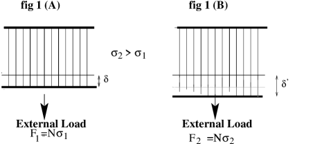
Figure 1: The vertical parallel lines correspond to fibers which are connected to two horizontal plates (shown with bold lines). The upper plate is fixed and the lower plate is movable. Fig. 1(a) shows a smaller force $F_{1}$ applied on the bundle producing a strain $\delta$. Fig. 1(b) corresponds to a higher value of load, leading to a strain $\delta^{{}^{\prime}}$ and fibers begin to break.

For a given force F, the fibers break and distribute their load following a load sharing rule until all the fibers have their threshold strength greater than the redistributed stress acting on them. This corresponds to the fixed point of the dynamics of the system. As the applied force is increased on the system, more and more fibers break and the additional stress is redistributed amongst the other fibers. There exist a critical load (or stress $\sigma_{c}$) beyond which if the load is applied, complete failure of the system takes place. Most of the studies on FBM involve the determination of the critical stress $\sigma_{c}$ and the investigation of the type of phase transition from a state of partial failure to a state of complete failure. It has been shown that a bundle following GLS has a finite value of critical stress and belongs to a universality class with a specific set of critical exponentsdynamic ; pratip whereas there is no finite critical stress $\sigma_{c}$ at thermodynamic limit in the case of LLS in one dimensionPacheco ; Hansen ; Smith ; reviewchak . On the other hand, LLS on complex network has been shown to belong to the same universality class as that of GLS with the same critical exponentscomplex .

The paper is organised as follows. Section II consists of mixed fibers with uniform distribution (UD) of threshold strength of fibers and GLS. The critical behaviour of such a model is explored analytically. Mixed fibers with Weibull distribution (WD) of threshold strength along with GLS is studied using a quasistatic approach of load increase in section III. One dimensional, one sided LLS with strictly uniform distribution (UD) is presented in section IV. Section V consists of a bundle of fibers whose tips are placed on a random graph with co-ordination number 3. The main conclusions are presented in section VI.

II Mixed Fibers with Uniform Distribution and GLS

Let us consider a ${}^{\prime}\rm mixed^{\prime}$ fiber bundle model with normalised density distribution of threshold strength as shown below:

Figure 2: Mixed Uniform Distribution.

$$\rho(\sigma_{th}) = \frac{1}{1-(\sigma_{2}-\sigma_{1})}~{}~{}~{}~{}~{}~{}0<\sigma_{th}\leq\sigma_{1}$$

$$= 0~{}~{}~{}~{}~{}~{}~{}~{}~{}~{}~{}~{}~{}~{}~{}~{}~{}~{}~{}~{}~{}~{}~{}\sigma_{1}<\sigma_{th}<\sigma_{2}$$

$$= \frac{1}{1-(\sigma_{2}-\sigma_{1})}~{}~{}~{}~{}~{}~{}~{}\sigma_{2}\leq\sigma_{th}\leq 1.$$ (1)

The present model clearly consists of fibers of two different types. This classification is based on whether a randomly chosen fiber from the bundle belongs to class A of fibers ($0<\sigma_{th}\leq\sigma_{1}$) or class B of fibers ($\sigma_{2}\leq\sigma_{th}\leq 1$) as shown in Fig. 2. In other words, the model consists of weak and strong fibers but no fibers with strengths between $\sigma_{1}$ and $\sigma_{2}$, which is the forbidden region for the fiber strength. Since we are considering GLS here, the exact location of class A or class B fibers is immaterial. The aim is to determine the critical stress $\sigma_{c}$ for this model such that if the external stress exceeds $\sigma_{c}$ , the bundle breaks down completely.

If a fraction $x$ of the total fibers belong to class A and the remaining $1-x$ to class B , then to maintain the uniformity of the distribution(Eq. (1)), we must have

$$\frac{1}{1-(\sigma_{2}-\sigma_{1})}\int_{0}^{\sigma_{1}}d\sigma=x$$

$$\frac{\sigma_{1}}{1-(\sigma_{2}-\sigma_{1})}=x$$

$$\noindent{\rm or},~{}~{}\sigma_{1}=\frac{x}{1-x}(1-\sigma_{2}).$$ (2)

The above equation provides the relationship between $x$, $\sigma_{1}$ and $\sigma_{2}$ showing that once $x$ and $\sigma_{1}$ are set, $\sigma_{2}$ is fixed automatically. This equation at the same time puts a restriction on $\sigma_{1}$. One can check that if $\sigma_{1}>x$, $\sigma_{2}$ becomes smaller than $\sigma_{1}$, which is impossible with the given form of distribution (Eq. (1)). We shall therefore restrict the value of $\sigma_{1}$ to be smaller than $x$.

The mechanism of the failure of RFBM is the following: under an external stress $\sigma$, a fraction of fibers having threshold strength less than the applied stress fail immediately. The additional load due to breaking of these fibers is redistributed globally among the remaining intact fibers. This redistribution causes further failures. Let us define $U_{t}=N_{t}/N$ as the fraction of unbroken fibers after a time step t. Then,

$$\sigma_{t}=\frac{F}{N_{t}}=\frac{\sigma}{U_{t}}.$$

The recurrence relation between $U_{t}$ and $U_{t+1}$ for a given applied stress $\sigma$ is obtained as dynamic :

$$U_{t+1}=1-P(\sigma_{t})=1-P(\frac{\sigma}{U_{t}}).$$ (3)

This dynamics propagate (in discrete time) until no further breaking takes place.

If the initial applied load is very small so that the redistributed stress is always less than $\sigma_{2}$, then no fibers from class B will fail. Thus for breaking of class B fibers, the redistributed stress has to be greater than $\sigma_{2}$. Let $\sigma_{t}$ (the redistributed stress) cross $\sigma_{2}$ at some instant t. Then the critical stress of the system can be calculated as follows:

$$U_{t+1} = 1-P(\frac{\sigma}{U_{t}})$$

$$= 1-[\frac{\sigma_{1}}{1-(\sigma_{2}-\sigma_{1})}+\frac{1}{1-(\sigma_{2}-\sigma_{1})}(\frac{\sigma}{U_{t}}-\sigma_{2})].$$

At fixed point of the dynamics, when no further breaking takes place, $U_{t+1}=U_{t}=U^{*}$ and we get,

$$U^{*}=1-[\frac{\sigma_{1}}{1-(\sigma_{2}-\sigma_{1})}+\frac{1}{1-(\sigma_{2}-\sigma_{1})}(\frac{\sigma}{U^{*}}-\sigma_{2})]$$

giving,

$$U^{*} = \frac{1}{2(1-(\sigma_{2}-\sigma_{1}))}[1\pm\sqrt{1-4[1-(\sigma_{2}-\sigma_{1})]\sigma}]$$

$$U^{*} = \frac{1}{2(1-(\sigma_{2}-\sigma_{1}))}[1\pm\sqrt{1-\frac{\sigma}{\sigma_{c}}]}$$ (4)

where

$$\sigma_{c}=\frac{1}{4[1-(\sigma_{2}-\sigma_{1})]}$$ (5)

It can be shown easily that the solution with $+$ in the parenthesis gives a stable solution. Therefore, $\sigma_{c}$ is the critical stress of the system because if the applied stress $\sigma$ is less than $\sigma_{c}$, the system reaches a fixed point. If the applied stress is greater than $\sigma_{c}$, $U^{*}$ becomes imaginary and the bundle breaks down completely. It is interesting to note that at $\sigma=\sigma_{c},~{}U^{*}=1/2[1-(\sigma_{2}-\sigma_{1})]$ $i.e.$, more than half of the fibers are still unbroken at critical point.

We should now look at the restrictions on $\sigma_{1}$, $\sigma_{2}$ and $x$ (other than $\sigma_{1}<x$) so that the above calculations are valid. From Eq. (4), we find that if the width of the forbidden region ($\sigma_{2}-\sigma_{1}$) is greater than half, $U^{*}(\sigma_{c})>1$ which is unphysical. Therefore, $(\sigma_{2}-\sigma_{1})$ should be smaller than 1/2 for all values of $x$ for the above calculations to hold. Using this restriction in Eq. (5), we find that the critical stress $\sigma_{c}$ will always be less than 1/2. Now, looking at the physical meaning of $U^{*}$, we must also check that the fraction of broken fibers at the fixed point corresponding to critical stress $\sigma_{c}$ must be greater than the fraction of fibers having their threshold stress smaller than the critical stress. We summarise all the restrictions below:

$$\sigma_{1}\leq x,~{}~{}\sigma_{2}-\sigma_{1}<0.5~{}~{}\rm and~{}~{}(1-U^{*}(\sigma_{c}))>P(\sigma_{c})$$ (6)

In the table below, we enlist some allowed values of $\sigma_{1}$, $\sigma_{2}$ for different $x$ and also the corresponding critical stress.

x	$\sigma_{1}$	$\sigma_{2}$	$\sigma_{c}$
0.10	0.08	0.28	0.31
0.20	0.19	0.24	0.26
0.30	0.25	0.42	0.30
0.30	0.29	0.33	0.26
0.40	0.35	0.47	0.29
0.50	0.45	0.55	0.27
0.80	0.7	0.82	0.28

From the table, we observe that the critical stress depends entirely on the width of the forbidden region, $i.e.$, $\sigma_{2}-\sigma_{1}$. Also, when $\sigma_{1}$ is increased for a fixed $x$, $\sigma_{2}$ decreases and hence $\sigma_{c}$ decreases. Physically, decreasing $\sigma_{2}$ (with $x$ fixed) means that lowest threshold of the strong fibers (class B) gets lowered. It is found that $\sigma_{1}$ cannot be very small compared to x, else all the above mentioned conditions do not get satisfied.

One can define an order parameter as shown below:

$$2[1-(\sigma_{2}-\sigma_{1})]U^{*}-1=(\sigma_{c}-\sigma)^{\frac{1}{2}}=(\sigma_{c}-\sigma)^{\beta}$$ (7)

The order parameter goes to 0 as $\sigma\rightarrow\sigma_{c}$ following a power law $(\sigma_{c}-\sigma)^{\frac{1}{2}}$ . Susceptibility can be defined as the increment in the number of broken fibers for an infinitesimal increase of load. Therefore,

$$\chi=\frac{dm}{d\sigma}~{}~{}~{}{\rm where}~{}~{}~{}m=N[1-U^{*}(\sigma)]$$

Hence,

$$\chi\propto(\sigma_{c}-\sigma)^{-\frac{1}{2}}=(\sigma_{c}-\sigma)^{-\gamma}$$ (8)

Figure 3: Variation of $\sigma_{c}$ with $\sigma_{2}-\sigma_{1}$ for a mixed RFBM with a distribution as in Fig. 2

As expected, the model follows mean field exponents with $\beta=1/2$ and $\gamma=1/2$. The interesting features of this model are: In this model, the forbidden zone has a nontrivial role to play. (i)By changing $(\sigma_{2}-\sigma_{1})$ and x, we can tune the strength of the system. However there are restrictions on the parameters as discussed above. $\sigma_{c}$ as a function of $(\sigma_{2}-\sigma_{1})$ is shown in Fig. 3. (ii) If x = 0, $\sigma_{2}\neq 0,\sigma_{1}=0(\rm~{}from~{}Eq.~{}2)$ which gives $\sigma_{c}=1/4(1-\sigma_{2})$ and we observe an elastic to plastic deformation as discussed in reference 9. In this case, for $\sigma<\sigma_{2}$, the fiber in the bundle obey Hook’s law. As soon as $\sigma>\sigma_{2}$, the dynamics of failure of fibers start. (iii)If $\sigma_{2}-\sigma_{1}$=0, the problem is that of a simple UD with threshold strength between 0 and 1 which has a critical stress $\sigma_{c}=0.25$ dynamic .

These results confirm that the failure of mixed fiber bundle model with Global Load Sharing belongs to a universality class with critical exponents $\beta=1/2$ and $\gamma=1/2$.

III Mixed Fibers with Weibull Distribution and GLS

In the Weibull distribution of threshold strength of fibers, the probability of failure of each element has the form

$$P(\sigma)=1-e^{-(\frac{\sigma}{\sigma_{0}})^{\rho}}$$ (9)

where $\sigma_{0}$ is a reference strength and $\rho$ is the Weibull index. We now consider a mixed RFBM as in section II with WD of threshold strength of fibers. As in the UD case (of Sec. (2)), here also a fraction $x$ of fibers belong to the class A (WD with $\rho=2$) and the remaining $(1-x)$ fraction belong to the class B (WD with $\rho=3$) with the reference strength $\sigma_{0}$ equal to 1 in either case.

For the conventional WD, consider a situation where the stress on each fiber increases from $\sigma_{1}$ to $\sigma_{2}$. The probability that a fiber randomly chosen from the WD survives from the load $\sigma_{1}$ but fails when the load is $\sigma_{2}$, is given by

$$p(\sigma_{1},\sigma_{2})=\frac{P(\sigma_{2})-P(\sigma_{1})}{1-P(\sigma_{1})}=1-e^{-(\sigma_{2}^{\rho}-\sigma_{1}^{\rho})}.$$

Thus the probability that the chosen fiber that has survived the load $\sigma_{1}$ also survives the (higher) load $\sigma_{2}$ is $q(\sigma_{1},\sigma_{2})=e^{-(\sigma_{2}^{\rho}-\sigma_{1}^{\rho})}$. The key point is that the force F on the bundle is increased quasistatically so that only one fiber amongst the remaining intact fibers break. As mentioned previously, the dynamics of breaking will continue till the system reaches a fixed point. The process of slow increase of external load is carried on up to the critical stress $\sigma_{c}$.

To deal with the nature of the present ${}^{\prime}\rm mixed^{\prime}$ random fiber bundle model, the method used by Moreno, Gomez and Pachecomixed3 is generalised in the following manner. It is important here to keep track of number of unbroken fibers in each distribution separately. Let us assume that after a loading is done and a fixed point is reached, $N_{k_{2}}$ and $N_{k_{3}}$ are the number of unbroken fibers corresponding to $\rho=2$ and $\rho=3$ distribution respectively, where each fiber has a stress $\sigma_{k}$.

Figure 4: Variation of fraction of broken fibers with external load per fiber $\sigma$ for a RFBM with two distributions corresponding to $\rho=2~{}\rm and~{}\rho=3$. N=50000, $x$=0.5

We define $q_{2}$ and $q_{3}$ as follows:

$$q_{2}(\sigma_{1},\sigma_{2})=e^{-(\sigma_{2}^{2}-\sigma_{1}^{2})}$$

$$q_{3}(\sigma_{1},\sigma_{2})=e^{-(\sigma_{2}^{3}-\sigma_{1}^{3})}.$$

The load $(N_{k_{2}}+N_{k_{3}})\sigma_{l}$ that has to be applied to break one fiber is given by $\sigma_{l}=min(\sigma_{l_{2}},\sigma_{l_{3}})$ where $\sigma_{l_{2}}$ (or $\sigma_{l_{3}}$) is the next weakest fiber in the $\rho=2$ (or $\rho=3$) distribution of strength of fibers and is obtained by the solution of the following equations.

$$N_{k_{2}}-1=N_{k{2}}q_{2}(\sigma_{k},\sigma_{l_{2}})$$

$$\noindent{\rm and}~{}~{}N_{k_{3}}-1=N_{k_{3}}q_{3}(\sigma_{k},\sigma_{l_{3}})$$

which gives

$$\sigma_{l_{2}}=[\sigma_{k}^{2}-{\rm ln}(1-\frac{1}{N_{k_{2}}})]^{1/2}$$ (10)

$$\sigma_{l_{3}}=[\sigma_{k}^{3}-{\rm ln}(1-\frac{1}{N_{k_{3}}})]^{1/3}$$ (11)

The breaking of one fiber and the redistribution of its stress causes some more failures. Let us say that during this avalanche, at some point before the fixed point is reached, there are $\widetilde{N_{k_{2}}}$ and $\widetilde{N_{k_{3}}}$ number of unbroken fibers belonging to the two distributions where each fiber is under a stress $\widetilde{\sigma_{k}}$. This stress causes some more failures and as a result $N_{k_{2}}^{{}^{\prime}}$ and $N_{k_{3}}^{{}^{\prime}}$ fibers are unbroken. Let the new stress developed is $\sigma_{k}^{{}^{\prime}}$. The number of fibers which survive $\widetilde{\sigma_{k}}$ and $\sigma_{k}^{{}^{\prime}}$ are obtained using the relation

$$N_{k_{2}}^{{}^{\prime\prime}}=N_{k_{2}}^{{}^{\prime}}q_{2}(\widetilde{\sigma_{k}},\sigma_{k}^{{}^{\prime}})$$ (12)

$$N_{k_{3}}^{{}^{\prime\prime}}=N_{k_{3}}^{{}^{\prime}}q_{3}(\widetilde{\sigma_{k}},\sigma_{k}^{{}^{\prime}})$$ (13)

The stress on each fiber is now equal to $(N_{k_{3}}^{{}^{\prime}}+N_{k_{2}}^{{}^{\prime}})\sigma_{k}^{{}^{\prime}}/(N_{k_{2}}^{{}^{\prime\prime}}+N_{k_{3}}^{{}^{\prime\prime}})$. Eq (12) and Eq. (13) are used again and again until a fixed point is reached. The fixed point condition is given by $(N_{k_{2}}^{{}^{\prime}}+N_{k_{3}}^{{}^{\prime}})-(N_{k_{2}}^{{}^{\prime\prime}}+N_{k_{3}}^{{}^{\prime\prime}})<\epsilon$ where $\epsilon$ is a small number (0.001). However, the critical behaviour does not depend on the choice of $\epsilon$.

After the fixed point is reached, stress $\sigma_{l}$ is calculated once again as mentioned before and the whole process is repeated till complete failure occurs at $\sigma_{c}$. The above mentioned approach has the advantage that it does not require the random averaging of Monte Carlo simulations.

Fig. 4 shows the fraction of total number of broken fibers as a function of applied stress $\sigma$ for the case $x=0.5$. The graph clearly shows the existence of a critical stress, $\sigma_{c}=0.46$, which lies between the critical stress of $\rho=2$ (0.42) and $\rho=3$ (0.49) distribution . These theoretical values are obtained from the analytical expression Daniel $\sigma_{c}=(\rho e)^{-1/\rho}$. The avalanche size S is defined as the number of broken fibers between two successive loadings. It diverges near the critical point with an exponent $\gamma=1/2$ as $(\sigma_{c}-\sigma)^{-\gamma}$. Scaling behaviour of avalanche size S is shown in Fig. 5. This confirms the mean field nature of GLS models even with mixed fibers. The most attractive feature of the mixed RFBM is shown in Fig. (6) which contains the variation of $\sigma_{c}$ with the fraction $x$ of class A fibers. Interestingly, $\sigma_{c}$ decreases linearly as $x$ is increased.

Figure 5: Scaling behaviour of avalanche size as the critical point is reached for the mixed model. Also shown is a straight line (dotted) with slope (-1/2). Here, N=50000 and $x=0.5$.

Figure 6: Variation of critical stress $\sigma_{c}$ with $x$. Slope of the straight line is 0.068. N=50000

IV One Dimensional, One sided LLS

In numerical studies, it is difficult to generate a strictly uniform distribution of the threshold strength of random fibers. In this work, we have addressed the problem of random fibers with UD of threshold with LLS scheme using an exact treatment of one sided load distributionPacheco . The complication arising in the present approach due to the uniform nature of the threshold distribution will also be emphasised later.

In one sided LLS, the additional load due to breaking of a fiber is transferred only to its neighbour in a given direction. The fibers are placed along the circumference of a circle with periodic boundary conditions. The method is based on the $k$-failure concept. If $k$ is chosen appropriately, then more than $k$ adjacent failures is equivalent to complete failure of the system. The scheme involved is as follows: let $p_{i}=p(\it{i\sigma}$) is the probability of failure of a fiber supporting a load $i\sigma$ (where $\sigma$ is the initial applied load per fiber). This is same as the probability of failure of all the previous $(\it{i}-1)$ fibers. Let $P_{N}(\sigma)$ represents the probability that a system of $N$ fibers break when an initial force equal to $N\sigma$ is applied and $Q_{N}(\sigma)=1-P_{N}(\sigma)$ is the probability that the bundle does not break because of initial load $N\sigma$. We have defined the critical load $\sigma_{c}$ by setting $P_{N}(\sigma_{c})=0.5$. However, any other choice of $P_{N}(\sigma_{c})$ does not alter the result. $Q_{N}(\sigma)$ can be easily identified as the probability that out of N fibers, there is no chain of adjacent broken fibers of length greater than $k$.

$Q_{N}(\sigma)$ can be calculated by using a simple iterative procedure described in Fig. 7.

Figure 7: Possible breaking configurations of a set with N=4 elements when the maximum allowed crack length is k=2 for one sided one dimensional LLS

The figure shows all possible states of a fiber in a system of 4 fibers with maximum number of allowed adjacent broken fibers equal to 2 (i.e., $k=2$). The notation means the following: the symbols 1 and 2 mean that in the corresponding position, the fiber breaks with a stress $1\sigma$, $2\sigma$ respectively. $1^{\prime},2^{\prime},3^{\prime}$ means that the corresponding element does not break under the stress $1\sigma$, $2\sigma$ and $3\sigma$ respectively. This simple notation can be extended to a system of $N$ fibers. If a fiber site has a symbol $m$, the two possibilities for the next fiber are $(m+1)$ and $(m+1)^{\prime}$. If the site has $m^{\prime}$, the two possibilities are $1$ and $1^{\prime}$ for the next site as $m^{\prime}$ means that the fiber has not broken and hence no additional stress is given to the next fiber. But if $m=k$, then the only allowed possibility for the fiber at the next site is $(k+1)^{\prime}$. This is to ensure that we are looking at only those configurations in which the complete breakdown does not take place. The aim is to write $Q_{N}(\sigma)$ in terms of $Q_{N-1}(\sigma)$. Let $B_{i}(N)$, where $i\leq k$ is the sum of probability contributions of the paths of length $N$ ending in the symbol i. Also, $B_{i^{\prime}}(N)$ with $i^{\prime}\leq k+1$, is the sum of contributions of all paths ending in symbol $i^{\prime}$. The following relations can then be obtained

$$B_{1}(N)=p_{1}\sum_{i=1}^{k+1}{B_{i^{{}^{\prime}}}}(N-1)$$ (14)

$$B_{i}(N)=p_{i}B_{i-1}(N-1),~{}~{}1<i\leq k$$

$$B_{1^{{}^{\prime}}}(N)=q_{1}\sum_{i=1}^{k+1}B_{i^{{}^{\prime}}}(N-1)$$

$$B_{i^{{}^{\prime}}}(N)=q_{i}B_{i-1}(N-1),~{}~{}~{}1<i^{{}^{\prime}}\leq k+1.$$

Thus $Q_{N}$ can be defined as

$$~{}~{}~{}~{}Q_{N}=\sum_{i=1}^{k}B_{i}(N)+\sum_{i=1}^{k+1}B_{i^{{}^{\prime}}}(N)$$ (15)

and hence the critical point can be obtained by demanding that $Q_{N}(\sigma)$ is 0.5 as the critical point is reached. B(N) can be written in a column matrix form where $B_{i}(N)$ and $B{i^{\prime}}(N)$ are its (2k+1) components. The set of equations represented by Eq.(14) can then be written as:

$$B(N)=M.B(N-1)$$ (16)

M can be identified as a square matrix with $(2k+1)^{2}$ components, all independent of N. M consists of the following elements:

$$\rm first~{}row~{}~{}M_{1,i}=0,~{}~{}~{}M_{1,i^{{}^{\prime}}}=p_{1}$$

$$\rm second~{}row~{}~{}M_{1^{{}^{\prime}},i}=0,~{}~{}~{}M_{1^{{}^{\prime}},i^{{}^{\prime}}}=q_{1}$$

rest of the rows:

$$M_{j,i}=\delta_{j-1,i}p_{j},~{}~{}~{}M_{j,i^{{}^{\prime}}}=0;$$

$$(i,j>1)~{}~{}~{}M_{j^{{}^{\prime}},i}=\delta_{j-1,i}q_{j},~{}~{}~{}M_{j^{{}^{\prime}},i{{}^{\prime}}}=0$$

where i=1,…k and $i^{{}^{\prime}}=1^{{}^{\prime}},2^{{}^{\prime}}.......,(k+1)^{{}^{\prime}}$.

Eq. (16) can now be written as:

$$B(N)=M^{N}B(1)$$ (17)

where vector $B(1)$ is given by $B_{i}(1)=\delta_{i,1}p_{1}$, and $B_{i^{{}^{\prime}}}(1)=\delta_{i^{{}^{\prime}},1^{{}^{\prime}}}q_{1}$

Since the model is based on the $k$-failure concept, the next question that arises is what an appropriate value for $k$ should be (which fixes the matrix size). This can be obtained by a simple criterion of convergence: if results do not vary when matrix size is increased from $k$ to $k+1$, then that value of $k$ is sufficient for $k$-failure concept. This is equivalent to saying that the probability of breaking when the stress on a fiber is $\it{(k+1)\sigma}$ is 1 (by the definition of $k$-failure)and hence there is no further change as one increases $k$(as the complete failure has already occurred).

Figure 8: The variation of $\sigma_{c}$ with $k$ for UD is shown in Fig 8(a).  Fig.  8(b) shows the variation of $1/\sigma_{c}$ with $\rm log_{2}N$.

The above described convergence can be clearly seen if one uses WD of threshold strengthPacheco . As mentioned before, the situation is different in the case of UD. The method used above allows the probability of failure to go beyond 1 if UD is used. The probability that a fiber breaks when the stress is $x\sigma$ is $x\sigma$, where $x$ should vary from 1 to $k$. It may happen that for some $x$ and $\sigma$, the matrix elements become greater than 1 which is clearly unphysical as each matrix element corresponds to a probability. It is observed that the value of $\sigma_{c}$ increases with $k$ and after attaining an almost constant $\sigma_{c}$, it starts decreasing. This decrease actually corresponds to the situation when the matrix elements at some stage of the calculation is either greater than 1 or less than 0 and hence not a saturation but a peak is obtained. Fig. 8(a) shows the variation of $\sigma_{c}$ with $k$ where a peak is observed. We have taken $k=8$ for our further calculations.

In Fig. 8(b), we have shown the variation of 1/$\sigma_{c}$ with log${}_{2}N$. Clearly it is a straight line which matches with the previously obtained analytical and numerical resultsPacheco ; Hansen ; Smith . The slope of the line is 0.81. The critical stress vanishes in the thermodynamic limit indicating the absence of a critical behaviour in one sided, one dimensional RFBM.

V Fibers on a random graph

Construct a random graph having $N$ sites such that each site has exactly 3 neighbours. The algorithm used is as follows: label the sites by integers from 1 to $N$ where $N$ is even. Connect site $i$ to $i+1$ for all $i$ such that site $N$ is connected to site 1. We call this connection as direct connection. Thus we have a ring of $N$ sites. Now connect each site randomly to a unique site other than $i+1$ and $i-1$, thus forming $N/2$ pairs of sites. This connection is called random connection. Each site in such a graph has a coordination number 3. In this construction, all sites are on the same footing (See Fig. 9). The tip of the fibers are placed on these $N$ sites and are associated with a UD of threshold strength.

Figure 9: An example of a random graph with coordination number 3 and 16 sites

Figure 10: The variation of $\pi$ with $\sigma$ for different values of $N$. Here, $N=2^{13},2^{14},2^{15},2^{16},2^{17},10^{5},2*10^{5}$. The lower $\sigma_{c}$ corresponds to a higher value of $N$.

The system is then exposed to a total load $N\sigma$ such that each vertex carries a stress $\sigma(i)=\sigma$. If $\sigma_{th}(i)<\sigma(i)$ at any site $i$, the fiber breaks and its stress is equally distributed to its surviving neighbours. The above condition is examined for each site and is repeated until there is no more breaking. Increase the total load $N\sigma$ to $N(\sigma+d\sigma)$. The new total load is then shared by the remaining unbroken fibers and once again the breaking condition is checked at each site. To make sure that the total load is conserved, if a fiber encounters a situation in which one of its neighbours is broken, it gives its stress to the next nearest surviving neighbour in that direction. This rule however is not applicable to the randomly connected fiber $i.e.$, if the randomly connected neighbour of a broken fiber is already broken, the stress then is given only to its directly connected neighbours. Once again, the load is increased and the process is repeated till complete breakdown of the system. In the numerical simulations, $d\sigma$ is taken to be 0.0001 and the average is taken over $10^{4}$ to $10^{5}$ configurations.

Fig. (10) shows the variation of $\pi$, the fraction of unbroken fibers, with stress $\sigma$ for different values of $N$. Clearly, there exist a non-zero value of critical stress even for large $N$.

To determine $\sigma_{c}$ precisely, we use the standard finite size scaling method Kim with the scaling assumption

$$\pi(\sigma,N)=N^{-a}f((\sigma-\sigma_{c})N^{\frac{1}{\nu}})$$ (18)

where f(x) is the scaling function and the exponent $\nu$ describes the divergence of the correlation length $\xi$ near the critical point, i.e., $\xi\propto|\sigma-\sigma_{c}|^{-\nu}$. If $\pi\propto(\sigma_{c}-\sigma)^{\beta}$, we obtain the relation $a=\beta/\nu$. The plots of $\pi N^{a}$with $\sigma$ for different N crosses through a unique point $\sigma=\sigma_{c}$=0.173 with the exponent $a=0.5$ (See Fig. 11).

Figure 11: Precise determination of $\sigma_{c}$ from the finite size scaling form (18). The $\sigma_{c}$ at which the curves intersect is 0.173

With this value of $\sigma_{c}$ and $a$, one can again use the scaling relation (18) to determine the exponent $\nu$ by making the data points to collapse to an almost single smooth curve as displayed in Fig. (12). The value of $\nu$ obtained in this manner is equal to 1 which automatically gives the value of the other exponent $\beta$=0.5. This matches with the mean field exponents derived analyticallydynamic . A random graph with connections as described above is equivalent to a Bethe lattice with co-ordination number $z$ ($=3$ in present case) for large N Dhar . It is observed that in this model, accurate value of $\sigma_{c}$(Fig. 11) and data collapse(Fig. 12) obtained by finite size scaling method is applicable in the limit of large N. It may be because of the resemblance of the underlying structure of the system with the Bethe lattice that it has mean field exponents. This should also be compared to Ising models with infinite-range interaction (which corresponds to GLS in the present context) Stanley and with short-range interaction on a Bethe lattice both showing mean field critical behaviour.

Figure 12: Data collapse with $a$=0.5, $\nu=1$

VI Conclusion

We have introduced a mixed RFBM with UD in one case and WD in the other within GLS scheme. The mixed RFBM with UD has a forbidden region $\sigma_{2}-\sigma_{1}$ so that the distribution of the threshold strength is discontinuous though the uniformity is ensured. The width of the forbidden region tunes the critical stress of the system and thus exhibits a rich critical behaviour. At the same time, restrictions on the parameters of the distribution for which the analytical method holds good are also clearly pointed out. The burst avalanche distribution of this type of discontinuous threshold distribution is expected to be very interesting and that is the subject of our further research. To study mixed RFBM with WD, a quasistatic approach is employed to determine the critical stress which decreases linearly with the fraction of class A fibers. Exponents obtained in both the above cases fall under mean field universality class. The most interesting feature of the mixed models is the tunability of the critical stress with the system parameters.

The behaviour of critical stress in a one dimensional RFBM with one sided LLS and strictly UD is also studied using an exact method and the complication arising due to the uniform nature of distribution is emphasized. We have also looked at the breakdown phenomena of RFBM on a random graph with coordination number 3. The critical stress is obtained using the finite size scaling method. The mean field nature of transition is established in the limit $N\to\infty$.

ACKNOWLEDGMENTS

The authors thank P. Bhattacharyya, S. M. Bhattacharjee, A. F. Pacheco and S. Pradhan for help and suggestions. Special thanks to Y. Moreno for helping us in writing a code and B. K. Chakrabarti for useful comments.

References

- (1) B. K. Chakrabarti and L. G. Benguigui, Statistical Physics of fracture and Breakdown in Disordered Systems, Oxford Univ. Press, Oxford (1997).
- (2) M. Sahimi, Heterogeneous Materials II: Nonlinear Breakdown Properties and Atomistic Modelling, Springer-Verlag Heidelberg, (2003).
- (3) H. J. Herrmann and S. Roux, Statistical Models of Disordered Media, North Holland, Amsterdam (1990)
- (4) P. Bak, How Nature Works, Oxford Univ. Press, Oxford (1997)
- (5) R. da Silveria, Am. J. Phys. 67, 1177 (1999)
- (6) F. T. Peirce, J. Text. Inst. 17, 355 (1926)
- (7) H. E. Daniels, Proc. R. Soc. London A 183 404 (1945)
- (8) B. D. Coleman, J. Appl. Phys. 29, 968 (1958)
- (9) S. Pradhan, P. Bhattacharyya and B.K. Chakrabarti, Phys. Rev. E66, 016116 (2002)
- (10) J. B. Gomez, D. Iniguez and A. F. Pacheco, Phys. Rev. Lett. 71, 380 (1993)
- (11) S.-D. Zhang, E.-J. Ding, Phys. Rev. B 53, 646 (1996)
- (12) B. Q. Wu and P. L. Leath, Phys. Rev. B 59, 4002 (1999)
- (13) Compare Ising Model with infinite range interaction, see for example, H. E. Stanley, Introduction to Phase Transitions and Critical Phenomenon, Oxford University Press, Oxford (1987)
- (14) R. C. Hidalgo, Y. Moreno, F. Kun and H.J. Herrmann, Phys. Rev. E 65, 046148 (2002)
- (15) S. Pradhan, B.K. Chakrabarti and A. Hansen, Phys. Rev. E 71, 036149 (2005)
- (16) P. Bhattacharyya, S. Pradhan and B.K. Chakrabarti, Phys. Rev. E67, 046122 (2003)
- (17) A. Hansen and P. C. Hemmer, Phys. Lett. A 184, 394 (1994)
- (18) R. L. Smith, Proc. R. Soc. London A 372, 539 (1980)
- (19) S. Pradhan and B. K. Chakrabarti, Int. J. Mod. Phys. B 17, 5565 (2003)
- (20) D. H. Kim, B. J. Kim and H. Jeong, Phys. Rev. Lett. 94, 025501 (2005)
- (21) Y. Moreno, J. B. Gomez and A. F. Pacheco, Phys. Rev. Lett. 85, 2865 (2000)
- (22) R. Albert, A.-L Barabasi, Rev. Mod. Phys. 74, 47 (2002)
- (23) B. J. Kim, Europhys. Lett. 66, 819 (2004)
- (24) D. Dhar, P. Shukla and J. P. Sethna, J. Phys. A: Math. Gen. 30,5259 (1997)
- (25) R. J. Baxter, Exactly Solved Models in Statistical Mechanics, Academic Press (1982)