Optical properties of small polarons from dynamical mean-field theory.

Abstract

The optical properties of polarons are studied in the framework of the Holstein model by applying the dynamical mean-field theory. This approach allows to enlighten important quantitative and qualitative deviations from the limiting treatments of small polaron theory, that should be considered when interpreting experimental data. In the antiadiabatic regime, accounting on the same footing for a finite phonon frequency and a finite electron bandwidth allows to address the evolution of the optical absorption away from the well-understood molecular limit. It is shown that the width of the multiphonon peaks in the optical spectra depends on the temperature and on the frequency in a way that contradicts the commonly accepted results, most notably in the strong coupling case. In the adiabatic regime, on the other hand, the present method allows to identify a wide range of parameters of experimental interest, where the electron bandwidth is comparable or larger than the broadening of the Franck-Condon line, leading to a strong modification of both the position and the shape of the polaronic absorption. An analytical expression is derived in the limit of vanishing broadening, which improves over the existing formulas and whose validity extends to any finite-dimensional lattice. In the same adiabatic regime, at intermediate values of the interaction strength, the optical absorption exhibits a characteristic reentrant behavior, with the emergence of sharp features upon increasing the temperature — polaron interband transitions — which are peculiar of the polaron crossover, and for which analytical expressions are provided.

I Introduction

The motion of electrons in solids is often coupled to the lattice degrees of freedom. There are broad classes of compounds where the electron-lattice interaction is such that the carriers can form small polarons, i.e. they are accompanied by a local lattice deformation that strongly modifies their physical properties, and can lead to the self-trapping phenomenon. This manifests in several experimentally accessible quantitiesAustin . First, the d.c. conductivity is thermally activated in a broad temperature range, with a gap related to the energy of the electron-lattice bound stateHolstein ; PRLrhopolaron . This is the energy barrier that the particle has to overcome to hop from site to site, which is proportional to the coupling strength. Second, most of the single-particle spectral weight — a quantity which is experimentally accessible through tunneling or photoemission spectroscopy — moves to high energies, corresponding to multi-phonon excitations in the polaron cloud AlexRann ; Mahan ; sumi ; depolarone ; Allen . Related to this, a broad contribution emerges in the optical conductivity, typically in the mid-infrared region, which can be ascribed to transitions inside the polaron potential-well old ; Reik ; Emin93 ; Mahan ; Firsov ; ray .

Besides the strength, the range and specific mechanism of electron-phonon coupling, the phenomenon of polaron formation depends on the properties of the host lattice, such as the dimensionality, the width of the conduction band and the frequency of phonon vibrations. In extremely narrow band systems, for example, the phonon energy can be of the order or even larger than the electronic bandwidth. This leads to the concept of antiadiabatic quasiparticles, that can move through the lattice being accompanied by a very fast phonon cloud, which is at the very basis of the standard small polaron treatments Holstein ; Lang-Firsov . In this framework, the small polaron optical absorption is strongly reminiscent of the behavior of electrons in a gas of independent molecules, and consists of a series of narrow peaks at multiples of the phonon frequency, whose distribution is determined by the electron-phonon coupling strength.

However, narrow band materials exist where the phonon frequency is appreciably smaller than the electronic bandwidth, which therefore cannot be described within the antiadiabatic approximation. In this case, one has to face the effect of the relatively large transfer integrals between molecules, which eventually wash out the discrete nature of the excitation spectra. Contrary to the antiadiabatic situation, where polaron formation occurs through a smooth crossover, in the adiabatic case a sharp transition separates the weak-coupling regime from the polaronic regime in dimensions greater than 1 Kabanov-Mashtakov ; Fehske-momentum ; xover . In the weak coupling limit, the optical absorption at low temperatures consists of an asymmetric band resulting from the excitation and absorption of a single phonon. In the strong coupling regime, the absorption spectrum moves to higher energies, reflecting the localized nature of the polaron. In this regime, provided that the free-electron bandwidth is small compared to the broadening of the Franck-Condon line, the optical absorption acquires a typical gaussian lineshape. old ; Reik In the opposite situation, i.e. when the electron dispersion dominates over the phonon-induced broadening, a different absorption mechanism sets in, corresponding to the photoionization of the polaron towards the free-electron continuum.Firsov ; ray To our knowledge, there is at present no satisfactory theory of the optical spectra in the regime where both mechanisms coexist, which is often the case in real experimental systems. Another important unsolved question, that cannot be addressed by standard methods, is how the optical absorption evolves between the weak and the strong coupling limit, and recent calculationsBRoptcond ; Fehske-opt have shown that the spectra in the intermediate coupling regime exhibit specific features that are characteristic of the polaron crossover region.

The simplest model which describes the rich phenomenology depicted above is the Holstein model Holstein , where tight-binding electrons are coupled locally to dispersionless bosons. The Holstein polaron problem can be solveddepolarone ; sumi in a non-perturbative framework using the dynamical mean field theory RMP (DMFT). While this method neglects the spatial dependence of the electron self energy, it treats exactly the local dynamics, which makes it particularly well suited to describe small polaron physics. It goes beyond the standard analytical approaches, as it can deal on the same footing with the low energy effective quasiparticles and the high energy incoherent features, which is crucial to the understanding of the polaron formation processdepolarone . The effects of a nonvanishing electron bandwidth and a nonvanishing phonon frequency are naturally included, which provides a unified description of the optical properties of small polarons, with no restrictions on the regimes of parameters. Compared to fully numerical methodsray ; Fehske-opt ; Fehske , which are also able to tackle the intermediate coupling regimes, the present approach is advantageous for the calculation of the optical conductivity, since it is free of finite size effects, and gives direct access to the electronic excitation spectrum in real frequency. In contrast, finite cluster diagonalization studies suffer from the discretization of the Hilbert space, which can be quite severe in the polaronic regime where many phonon states are needed, while quantum Monte Carlo treatments usually work in imaginary time, and rely on analytical continuation algorithms for the extraction of spectral and optical properties. Note however that the present DMFT results, which are based on an exact continued fraction expansion in the low density limit,depolarone cannot be directly generalized to finite densities.

The aim of this work is to take advantage of the DMFT to address the regimes of parameters not covered by the standard formulas of small polaron theory. Applying this non-perturbative method, we can critically examine the ranges of validity of the usual limiting approximations, and point out the quantitative and qualitative discrepancies arising in several regions of the parameters space. Special emphasis is given to the following points, which are not accessible by the usual methods available in the literature: i) the evolution of the multi-peaked spectra in the antiadiabatic regime, at finite values of the free-electron bandwidth; ii) the effects of a finite electron dispersion on the usual Franck-Condon lineshapes, in the adiabatic polaronic regime; iii) the peculiar features arising in the region of the adiabatic polaron crossover. Concerning the last point, the results of our previous work Ref.BRoptcond , where such features were first reported, are here extended to much lower temperatures, which is made possible by a new adaptive method introduced to deal with the fragmented excitation spectra characteristic of the polaron problem. depolarone This new procedure allows to identify a reentrant behavior of the optical properties in the crossover regime, where increasing the temperature switches from a weak-coupling like absorption to a typical polaronic lineshape. Furthermore, a previously published formula for the $T=0$ absorption in the polaron crossover regime is corrected here, and analytical expressions are derived to describe the lineshape of the polaron interband transitions reported in Ref.BRoptcond .

The paper is organized as follows: In Section II we introduce the DMFT formalism and the Kubo formula for the optical conductivity, and discuss the details of the calculations. Sections III and IV are devoted to the analysis of the absorption spectra respectively in the antiadiabatic and in the adiabatic regimes. The specific features arising at intermediate values of the coupling strength in the adiabatic polaron crossover region are examined in Section V. The main results are summarized in Section VI.

II Model and formalism

We study the Holstein hamiltonian, where tight-binding electrons ($c_{i,\sigma},c_{i,\sigma}^{\dagger}$) with hopping amplitude $t$ are coupled locally to Einstein bosons ($a_{i},a_{i}^{\dagger}$) with energy $\omega_{0}$:

$$H = \omega_{0}\sum_{i}a^{+}_{i}a_{i}-g\sum_{i,\sigma}c^{+}_{i,\sigma}c_{i,\sigma}(a^{+}_{i}+a_{i})$$ (1)

$$- t\sum_{i,j,\sigma}\left(c^{+}_{i,\sigma}c_{j,\sigma}+{\rm H.c.}\right).$$

The single polaron problem can be solved in the framework of the DMFTRMP , which yields an analytical expression for the local self-energy $\Sigma(\nu)$ in the form of a continued fraction expansionsumi ; depolarone . The latter must be iterated in an appropriate self-consistent scheme, where the free-electron dispersion defined by the tight-binding term in Eq. (1) enters only through the corresponding density of states (DOS) $N(\epsilon)$. From the knowledge of the self-energy, one can define the single particle spectral function

$$\rho(\epsilon,\nu)=-\frac{1}{\pi}Im\frac{1}{\nu-\Sigma(\nu)-\epsilon}$$ (2)

that carries information on the spectrum of excited states, and its momentum integral, the spectral density $N^{*}(\nu)$. The latter can be evaluated by introducing the Hilbert transform of the DOS, ${\cal H}(z)=\int d\epsilon N(\epsilon)/(z-\epsilon)$ as:

$$N^{*}(\nu)=-(1/\pi)\ Im\ {\cal H}[\nu-\Sigma(\nu)].$$ (3)

The conductivity at finite frequency is related to the current-current correlation function through the appropriate Kubo formula. In DMFT, due to the absence of vertex correctionsDINF-OC ; RMP , such two-particle response function can be expressed as a functional of the fully interacting single particle spectral function $\rho(\epsilon,\nu)$ (or, equivalently, of the local self-energy $\Sigma$). This can be related to the single polaron solution of Ref. depolarone by performing an expansion in the inverse fugacity BRoptcond $z^{-1}=\exp(\mu/T)$. ($z^{-1}\to 0$ as the chemical potential $\mu\to-\infty$ in the limit of vanishing density at any given temperature). The optical conductivity turns out to be proportional to the carrier concentration $x$, and can be expressed in compact form as

$$\sigma(\omega)=\frac{x\zeta\pi}{\omega}(1-e^{-\beta\omega})\frac{{\cal D}(\omega,\beta)}{{\cal N}(\beta)}$$ (4)

where the constant $\zeta=e^{2}a^{2}/\hbar v$ carries the appropriate dimensions of conductivity ($a$ being the lattice spacing, $v$ the volume of the unit cell) and $\beta=1/T$ is the inverse temperature. We have defined

$${\cal D}(\omega,\beta) = \int d\epsilon N(\epsilon)\phi(\epsilon)\times$$

$$\times\int d\nu e^{-\beta(\nu-E_{0})}\rho(\epsilon,\nu)\rho(\epsilon,\nu+\omega)$$

$${\cal N}(\beta) = \int d\nu e^{-\beta(\nu-E_{0})}N^{*}(\nu)$$ (6)

where $E_{0}$ is the polaron ground state energy at $T=0$. The exponential factors account for the thermal occupation of the electronic levels (the Fermi temperature vanishes in the low density limit, and the particles obey Maxwell-Boltzmann statistics). The normalization factor ${\cal N}$ represents the partition function of the interacting carrier. Unless differently specified, the density of states $N(\epsilon)$ of the unperturbed lattice, that enters in the definition of the correlation function ${\cal D}$, is assumed semi-elliptical of half bandwidth $D$

$$N(\epsilon)=\frac{2}{\pi D^{2}}\sqrt{D^{2}-\epsilon^{2}}$$ (7)

corresponding to a Bethe lattice in the limit of infinite connectivity. This choice reproduces the low energy behavior of a three-dimensional lattice, while leading to tractable analytical expressions. The function $\phi(\epsilon)$ is the corresponding current vertex

$$\phi(\epsilon)=(D^{2}-\epsilon^{2})/3$$ (8)

that can be derived by enforcing a a sum rule for the total spectral weight Freericks ; Millis . Compared to the more rigorous procedure of Ref. Vandongen , this has the advantage of leading to the correct threshold behavior for the optical conductivity expected in a three-dimensional system in the weak coupling limit,Mahan as well as in the adiabatic photoionization limit,Emin93 ; Firsov ; ray as will be shown below. In the usual strong coupling regime,old ; Reik on the other hand, the results become independent on the detailed shape of both $N$ and $\phi$, and the choice of the vertex function is not influent. Let us mention that low-dimensional systems can also be studied with the present method, by replacing $N(\epsilon)$ and $\phi(\epsilon)$ of Eqs. (7) and (8) with the appropriate DOS and vertex function. In such cases, the neglect of vertex corrections in the current-current correlation function that is implicit in the DMFT formulation could in principle constitute an important limitation. In practice, however, the limiting cases of weak and strong coupling are correctly reproduced by the DMFT, which gives some confidence on the results obtained in more general situations (see e.g. the discussion at the beginning of Section IV A).

With the present choice of Eqs. (7) and (8), the Hilbert transform ${\cal K}(z)$ of the product $N(\epsilon)\phi(\epsilon)$ can be expressed in closed form, which allows the $\epsilon$-integral in Eq. (II) to be performed explicitely:

$${\cal D}=\int d\nu e^{-\beta(\nu-E_{0})}B[\omega+\nu-\Sigma(\omega+\nu),\nu-\Sigma(\nu)]$$ (9)

with

$$B(z_{1},z_{2})=-\frac{1}{2\pi^{2}}Re\left[\frac{{\cal K}(z_{1})-{\cal K}(z_{2})}{z_{2}-z_{1}}-\frac{{\cal K}(z_{1}^{*})-{\cal K}(z_{2})}{z_{2}-z_{1}^{*}}\right].$$

The remaining integral in $\nu$ appearing in Eq. (9) has to be computed numerically, which presents two main difficulties. First of all, at temperatures $T\ll\omega_{0}$, the function $B\propto Im\Sigma(\nu)$ decays exponentially at energies $\nu$ below the ground state $E_{0}$. Nevertheless, such regions contribute to the final result due to the presence of the thermal factor $e^{-\beta(\nu-E_{0})}$. As a rule of thumb, at low temperatures, the integration limits must be extended down to $\nu-E_{0}\simeq-2E_{P}$ to account for a proper number of excited states . At the bottom of the integration region, the number $B$ is therefore multiplied by an exponentially large factor $e^{2E_{P}/T}$ which amplifies the numerical errors and, for typical values of $E_{P}/\omega_{0}\sim 10$, limits the attainable low temperature limit to $T/\omega_{0}\sim 0.1$. The second difficulty is that, in the strong coupling regime, the function $B$ is zero almost everywhere for $\nu<E_{0}$, being concentrated in exponentially narrow peaks of width $\sim e^{-E_{P}/\omega_{0}}$, corresponding to multi-phonon resonances at multiples of $\omega_{0}$ (see Fig. 5 below). For example, taking the parameters of Fig. 3.b, the ratio between the width of the peaks and their separation is $10^{-3}$. Special care must be taken to manage with this rapidly varying function. A uniform mesh discretization of the integral appearing in Eq. (9) was used in Ref. BRoptcond , which was appropriate for the intermediate coupling/temperature regimes. To attain the strong coupling and low temperature regimes, we use here an adaptive non-uniform mesh optimized to account for the narrow peaks of the function $e^{-\beta(\nu-E_{0})}Im\Sigma(\nu)$.

Bearing these limitations in mind, we shall present in the following Sections the numerical results for coupling strengths up to $E_{P}/\omega_{0}\sim 10$ and temperatures down to $T/\omega_{0}\sim 0.01-0.1$ (the lowest temperatures are reached in the weak/intermediate coupling regime). Analytical formulas will be derived to access the limits of strong coupling and vanishing temperatures. For simplicity, we shall drop the numerical prefactor $x\zeta$ in Eq. (4) and express all energies in units of the half-bandwidth $D$.

III Optical conductivity in the antiadiabatic regime

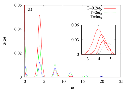
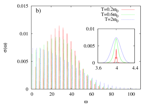
Figure 1: (Color online) Optical conductivity in the antiadiabatic regime, a) for $\gamma=\omega_{0}/D=4$ and $\alpha^{2}=0.25$ and b) $\alpha^{2}=5$. a) In the weak coupling regime, the individual absorption peaks shrink upon increasing the temperature above $T\sim\omega_{0}/2$, as predicted by Holstein’s approximation. In the inset, the low-temperature evolution of the one-phonon absorption is shown (full red lines, from left to right, $T/\omega_{0}=0.2,0.05,0.02$). The black dotted line is the weak coupling result (10) at $T=0$. The absorption edge shifts from $\omega=\omega_{0}-2D$ at $T\gtrsim D$ to $\omega=\omega_{0}$ at $T\ll D$ (see appendix A). b) In the strong coupling regime, the optical absorption consists of extremely narrow peaks, similar to the case of an isolated molecule (the peaks at $T=0.6\omega_{0}$ and $T=2\omega_{0}$ have been shifted laterally by a constant offset for clarity). Contrary to the weak coupling limit, here the individual peaks broaden with temperature (see inset).

The process of polaron formation at zero temperature is different depending on the value of the adiabaticity ratio $\gamma=\omega_{0}/D$, which measures the relative kinetic energies of phonons and band electrons ($D$ is half the free-electron bandwidth, proportional to the hopping amplitude $t$). In the antiadiabatic regime ($\gamma\gg 1$), the buildup of electron-lattice correlations occurs through a smooth crossover controlled by the coupling parameter $\alpha^{2}=E_{P}/\omega_{0}$, depolarone ; xover which sets the average number of phonons in the polaron cloud ($E_{P}\equiv g^{2}/\omega_{0}$ is defined as the polaron binding energy on an isolated molecule). In this case the behavior of the optical absorption at any value of the electron-phonon coupling strength can be deduced to a good approximation from the analysis of an isolated molecule, corresponding to the limit $D\to 0$. old ; Reik ; Mahan It consists of a series of narrow peaks at multiples of $\omega_{0}$, whose distribution is determined by the coupling parameter $\alpha^{2}$, and evolves gradually through the polaron crossover located around $\alpha^{2}\sim 1$ (see also Fig. 2 in the following). At low $\alpha^{2}$, the spectral weight is mainly located in the Drude peak, plus a weaker absorption peak at $\omega=\omega_{0}$. Upon increasing the coupling strength, multiphonon scattering processes become important, and several peaks arise at multiples of $\omega_{0}$. For $\alpha^{2}\gg 1$, the distribution of the peak weights eventually tends to a gaussian centered at $\omega=2E_{P}=2\alpha^{2}\omega_{0}$, with a variance $\sim\sqrt{2E_{P}\omega_{0}}$ [cf. App. A and Eq. (12) below].

Thermal effects lead to some redistribution of spectral weight among the different peaks: In the weak coupling regime, the thermal excitation of phonons generates additional absorption peaks at multiples of $\omega_{0}$. In the strong coupling regime, increasing the temperature broadens the distribution of peak weights: For $T\gtrsim\omega_{0}/2$, the variance tends to $\sqrt{4E_{P}T}$ and is completely determined by the thermal fluctuations of the phonons (cf. App. A); When the temperature is increased further, thermal dissociation of the polaron at $T\sim E_{P}$ eventually washes out the absorption maximum at finite frequency, resulting in a transfer of spectral weight towards $\omega=0$.

The above picture is based on the limit of vanishing electron bandwidth. A small nonvanishing transfer integral can be expected to give the individual peaks a finite width, without modifying the distribution of spectral weights AlexRann . In the weak coupling regime, this scenario is confirmed by the DMFT results illustrated in Figure 1.a for $\gamma=4$ and $\alpha^{2}=0.25$. The absorption spectrum at $T=0.2\omega_{0}$ consists of few peaks of width $\simeq 4D$, centered at multiples of $\omega_{0}$; Increasing the temperature leads to a moderate transfer of spectral weight to higher frequencies, while the individual peaks shrink as predicted by Holstein’s approximationHolstein . An interesting behavior is seen at extremely low temperatures, where $T\ll D\ll\omega_{0}$ (inset of fig 1.a). In this limit, the optical absorption is dominated by transitions between “low momentum” states, i.e. states located near the bottom of the subbands. As a result, the peaks become asymmetric and the absorption thresholds move from $\omega=n\omega_{0}-2D$ to $\omega=n\omega_{0}$ [details are given in Appendix A, Eq. (25) and (26)].

The optical conductivity in the strong coupling regime ($\gamma=4$ and $\alpha^{2}=5$) is shown in Fig. 1.b. In this case, although the overall picture deduced from the molecular limit is qualitatively recovered, the fine structure exhibits a behavior that contradicts the standard results available in the literatureHolstein ; Reik ; AlexRann ; Lang-Firsov , according to which the absorption spectra at nonzero $D$ consist of a series of narrow peaks of equal width, proportional to the renormalized polaronic bandwidth [this follows, through Eq. (II), from the assumption that the multiphonon subbands in the single particle spectral density all have the same width]. Instead, the multiphonon peaks in Fig. 1.b are broader at high frequency than at low frequency, although this is hardly visible on the scale of the figure. More surprisingly, their width increases with temperature, as shown in the inset of Fig. 1.b, contrary to what could be expectedHolstein .

This apparently anomalous behavior can be traced back to finite bandwidth effects on the excitation spectrum, that go beyond Holstein’s decoupling scheme, and have already been reported in Ref. depolarone as well as in Ref.PRLrhopolaron , where they have been shown to strongly affect the absolute value of the d.c. conductivity. In fact, the broadening of molecular levels induced by band overlap is not uniform over the excitation spectrum, but rather increases as they move away from the groud state (see e.g. Figs. 17 and 18 in Ref. depolarone ): while the width of the lowest peak, related to coherent tunneling between different molecular units, scales exponentially as $\exp(-\alpha^{2})$, the width of the higher order peaks is much larger, being determined by both incoherent hopping between neighboring molecules and coherent hopping in the presence of multiphonon excited states: for such peaks, the DMFT results indicate a power law dependence in $\alpha^{2}$. Moreover, as the temperature increases, the different levels are mixed by phonon thermal fluctuations. As a result, the width of the subbands at low energy rapidly increases with temperature to attain the typical broadening of the high energy subbands, as seen in the inset of Fig. 1.b (in the data at $T=0.2\omega_{0}$, a fine structure due to the superposition of at least two contribtions of different widths is visible).

Note that the discrete multi-peaked structure characteristic of the antiadiabatic regime remains at all temperatures, contrary to what is stated in Ref. Reik : when $D\ll\omega_{0}$, the thermal broadening of the peaks is not sufficient to lead to a continuous absorption curve, even at $T\gg E_{P}$, unless a sizeable phonon dispersion is introduced in the model (this would give the individual peaks an intrinsic finite width, preventing the extreme band narrowing in the limit $D\to 0$).

IV Optical conductivity in the adiabatic regime

In the adiabatic limit ($\gamma=0$), the carrier properties change drastically from weakly renormalized electrons to self-trapped polarons at a critical value of the coupling strength $\lambda\equiv E_{P}/D$, above which a bound state emerges below the bottom of the free-electron band. For example, in the case of the semi-elliptical density of states Eq. (7), adiabatic polaron formation takes place at $\lambda_{c}=0.843$. Allowing for lattice quantum fluctuations changes this localization transition into a very sharp crossover (cf. Fig. 2) which separates weakly renormalized electrons for $\lambda\lesssim\lambda_{c}$ from polarons with very large effective mass at $\lambda\gtrsim\lambda_{c}$. depolarone ; xover

To describe this behavior, methods such as the DMFT that do not rely on a “small” parameter are extremely valuable for the following reasons. On one hand, there is at present no unified analytical approach which allows to calculate the optical conductivity (even approximately) in the whole range of parameters, from the weak to the strong coupling limit. This is not surprising, since the physics is fundamentally different in the two regimes. This situation should be contrasted with the antiadiabatic case, where the basic qualitative features of the optical absorption can be inferred form the solution of the model on a single molecule (cf. beginning of Section III A). In addition, even within the adiabatic strong coupling regime, the polaronic lineshape changes depending on the ratio between the broadening $s$ of electronic levels induced by phonon fluctuations, and the free electron bandwidth $D$. Theories exist for the limits $s/D\to 0$ and $s/D\to\infty$, but their validity is questionable in the intermediate range of experimental relevance.

In the following, we shall first report the analytical expressions recovered within the present DMFT formalism, in three limiting cases: weak coupling, strong coupling $s/D\to\infty$ and $s/D\to 0$. The first two formulas turn out to be perfectly equivalent to the results available in the literature, showing that at least in such limits, the neglect of vertex corrections in the Kubo formula implicit in the DMFT approach has negligible influence on the results. The third formula, on the other hand, constitutes an improvement over the expressions of Refs. Firsov ; ray , even when applied to one-dimensional lattices. The DMFT results obtained in more general cases will be presented next, pointing out the inadeguacy of the standard descriptions in many cases of interest.

IV.1 Limiting cases

In the weak coupling limit ($\lambda\to 0$), the optical absorption at $T=0$ consists of a broad band related to the excitation of a single-phonon, with an edge at $\omega=\omega_{0}$ followed by a power law decay at higher frequencies, and eventually an upper edge at $\omega=\omega_{0}+2D$ [cf. Eq. (25) in Appendix A]

$$\sigma(\omega)=\frac{E_{p}\omega_{0}\pi}{\omega^{3}}\phi(\omega-D-\omega_{0})N(\omega-D-\omega_{0}).$$ (10)

In a three dimensional system, the absorption edge behaves as $(\omega-\omega_{0})^{3/2}$. As the temperature increases, the gap below the threshold is rapidly filled and the absorption maximum is washed out above $T\sim\omega_{0}/2$.

In the strong coupling regime ($\lambda\to\infty$), the photoexcitation of the electron is much faster than the lattice dynamics, which is virtually frozen during the absorption process. Since the lattice energy cannot be relaxed, the dominant optical transition corresponds to the difference in electronic energy between the initial and final states (Franck-Condon principle) which, in the Holstein model, equals twice the ground state energy $2E_{P}$. The shape of the optical absorption will depend on the ratio between the width of the non-interacting band $\sim D$, and the variance $s$ of the phonon field, which controls the broadening of electronic levels. The latter obeys HoHu

$$s^{2}=E_{P}\omega_{0}\coth{\omega_{0}/2T}$$ (11)

(cf. Appendix A). It is determined by the quantum fluctuations of the phonons at low temperatures, and increases due to the thermal fluctuations as $T\gtrsim\omega_{0}/2$.

When $s\gg D$, i.e. when the phonon induced broadening of electronic levels is much larger than the electronic dispersion, the absorption by localized polarons takes the form of a skewed gaussian peak centered at $\omega_{max}=2E_{P}$: old ; Reik

$$\sigma(\omega)=\frac{\pi}{\omega}\frac{D^{2}}{4}\frac{1-e^{-\omega/T}}{\sqrt{4\pi s^{2}}}\exp\left[-\frac{(\omega-2E_{P})^{2}}{4s^{2}}\right].$$ (12)

Following Eq. (11), the Franck-Condon line further broadens upon increasing the temperature above $T\sim\omega_{0}/2$ and eventually moves towards $\omega=0$ at temperatures higher than the polaron binding energy, as the polaron thermally dissociates. Note that the above formula also describes the envelope of the discrete absorption spectrum of polarons in the antiadiabatic regime, shown in the preceding Section (cf. Fig. 1.b).

To recover the standard result for a three-dimensional cubic lattice,Mahan where the total bandwidth is $2D=12t$, the above formula has to be multiplied by a prefactor $2/9$, which corrects for the larger value of the average square velocity in the DOS Eq. (7) used in the calculations. Analogous prefactors should be included when any of the DMFT results obtained in this work are applied to finite-dimensional lattices, that can be straightforwardly obtained by evaluating the second moment of the corresponding non-interacting DOS.

In the opposite limit $s\ll D$, the lineshape is dominated by the electronic dispersion. The absorption is due to transitions from a polaronic state whose electronic energy is $\simeq-2E_{P}$ to the continuum of free-electron states. We have [cf. Eq. (36) in Appendix A]

$$\sigma(\omega)=\pi\frac{4E_{P}^{2}}{\omega^{2}}\frac{1-e^{-\omega/T}}{\omega}\phi(\omega-2E_{P})N(\omega-2E_{P})$$ (13)

We see that in this case the absorption of photons is only possible in the interval $2E_{P}-D<\omega<2E_{P}+D$. In three dimensions, the absorption vanishes as $\Delta\omega^{3/2}$ at the edges, as in the weak coupling case of Eq. (10). Taking a semi-elliptical DOS as representative of a three-dimensional lattice, we also find that the absorption maximum $\omega_{max}=2E_{P}-D^{2}/2E_{P}$ is shifted to lower frequencies compared to the usual estimate. This softening is entirely due to finite bandwidth effects. Note that Eq.(13) is valid at all temperatures below the polaron dissociation temperature $T\sim E_{P}$. In particular, contrary to Eq. (12), nothing happens here at temperatures $T\sim\omega_{0}/2$, provided that the condition $s\ll D$ is not violated.

Formulas similar to Eq. (13) have been derived in Ref. Firsov , in Ref. ray for one-dimensional systems, and in Ref. Emin93 for the high frequency absorption threshold of large polarons in the Fröhlich model. As discussed in Appendix A, these derivations are strictly valid only in the limit $E_{P}\to\infty$. On the other hand, the present formula accounts for the non-negligible dispersion of the initial state at finite values of $E_{P}$, which is reflected in the additional prefactor $4E_{P}^{2}/\omega^{2}$, leading in general to a much more asymmetric lineshape. Remarkably, if the appropriate one-dimensional DOS is used, Eq. (13) describes much better the one-dimensional exact diagonalization data of Ref. ray than their own Eq. (9) [also reported in Appendix A as Eq. (33)]. The absorption maximum in this case is located at $\omega_{max}=2E_{P}-E_{P}(\sqrt{1+6(D/E_{P})^{2}}-1)/2$.

The regions of validity of the analytical formulas presented in this Section are summarized in Fig. 2.

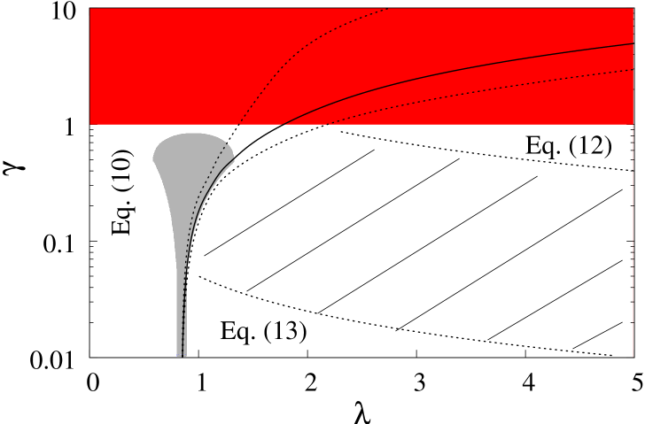
Figure 2: (Color online) Phase diagram illustrating the regimes of validity, at $T=0$, of the different limiting formulas derived in the text. The bold and dotted lines indicate the location and spread of the polaron crossover as defined in Ref.xover . The (red) shaded region delimits the antiadiabatic regime $\gamma>1$ treated in Section III. In the hatched region at $\gamma<1$, the optical conductivity is not accessible by the usual methods, as pointed out in Section IV. The (gray) shaded region indicates the adiabatic intermediate regime described in Section V.

IV.2 DMFT results

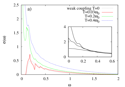
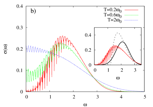
Figure 3: (Color online) Optical conductivity in the adiabatic regime, a) $\gamma=\omega_{0}/D=0.1$ and $\lambda=0.7$ and b) $\lambda=1.1$. a) In the weak coupling regime, the gap below $\omega=\omega_{0}$ is rapidly filled upon increasing the temperature, and the one-phonon absorption threshold is washed out at $T\gtrsim\omega_{0}/2$. The black dotted line is the analytical weak-coupling result (10). At higher temperatures, the low-frequency absorption is reduced as some spectral weight is transferred to higher frequencies (see inset: from top to bottom, $T/\omega_{0}=0.4,0.6$ and $1$). b) In the polaronic regime, the absorption peak broadens at $T\gtrsim\omega_{0}/2$ and then moves towards $\omega=0$ as $T\gtrsim E_{P}$. The inset compares the low temperature spectrum with the limiting lineshapes Eq. (12) (full line) and Eq. (13) (dashed line).

The DMFT results obtained in the adiabatic regime are illustrated in Fig. 3. First of all, our data show that the absorption shape (10) derived in the limit of $\lambda\to 0$ remains qualitatively valid at finite values of $\lambda$, up to the polaron crossover. This is exemplified in the data reported in Fig. 3.a. at $\gamma=0.1$ and $\lambda=0.7$, i.e. at a value of the coupling strength which lies a priori well beyond the range of validity of perturbation theory, xover not far from the polaron crossover coupling strength $\lambda_{c}(\gamma=0.1)\simeq 0.93$ (see Fig. 2 and Section V below). Despite such relatively large $\lambda$, the threshold at $\omega_{0}$ and the overall behavior of the high frequency tail at low temperatures (full red line) are quite close to the predictions of the weak-coupling formula (10) (black, thin dotted line). The increasing importance of multi-phonon processes shows up mainly in the fine structure, with the appearance of alternating peaks and dips at multiples of $\omega_{0}$.

Figure 3.b shows the DMFT results at $\gamma=0.1$ and $\lambda=1.1$. This value of the coupling strength lies in the polaronic regime $\lambda>\lambda_{c}$, in a region where the electronic dispersion and the phonon-induced broadening are comparable ($s/D=0.33$), so that none of Eqs. (12) and (13) is expected to hold. The comparison with such limiting formulas is illustrated in the inset of Fig. 3.b. While the position of the absorption maximum seems to agree with the prediction of Eq. (13) (dashed line), the peak height is much reduced and the absorption edge is completely washed out by phonon fluctuations. On the other hand, the temperature dependence qualitatively agrees with Eq. (12) (full line), i.e. the peak broadens as the temperature is raised above $T\sim\omega_{0}/2$, which can be understood because the low frequency tails are dominated by the phonon fluctuations. We see that the DMFT spectrum not only lies at lower frequencies compared to Eq. (12), but it is also much broader and asymmetric (the same trend was observed in Ref.Fehske-opt in the one-dimensional case). All these effects can be ultimately ascribed to the finite electron bandwidth $D$.

Our results show that detectable deviations from Eq. (12) arise as soon as the non-interacting bandwidth is larger than the broadening $s$, a condition that is commonly realized in real systems. For example, taking typical values $\omega_{0}\simeq 0.01-0.05eV$ and $E_{p}\simeq 0.1-0.5eV$ yields a zero temperature broadening $s\simeq 0.03-0.16eV$, in which case electron bandwidths of few tenths of $eV$ are already sufficient to invalidate the standard gaussian lineshape Eq. (12). In the opposite limit, marked deviations from Eq. (13) appear already at small values of the ratio $s/D$, roughly $s/D\gtrsim 0.05$: as soon as a small finite broadening is considered, exponential tails of width $s$ arise that wash out the sharp absorption edge of Eq. (13), while the peak height is rapidly reduced (this can be partly ascribed to a rigid increase of the renormalized band dispersion, as evidenced in Ref. HoHu ). The intermediate region where both Eq. (12) and (13) fail in describing the polaronic optical absorption is shown as a hatched area in Fig. 2.

As was mentioned above, the ability to describe the continuous evolution of the absorption shape between the limiting cases of Eq. (12) and Eq. (13) ultimately follows from the fact that finite bandwidth effects are properly included in the DMFT. On the other hand, accounting for a non-zero phonon frequency allows to address the multi-phonon fine structure of the optical spectra, which is seen to evolve gradually upon varying the adiabaticity ratio $\gamma$. In fact, the optical absorption of a polaron at finite values of $\gamma$ shares features with both the antiadiabatic and adiabatic limits, having a pronounced structure at low frequencies (possibly with multiple separate narrow bands), followed by structureless tails at higher frequencies (cf. Fig. 3.b). As $\gamma$ increases, the fine structure progressively extends to higher frequencies, and evolves into the discrete absorption pattern of Fig. 1.b, typical of the antiadiabatic limit.

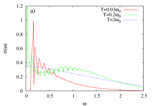
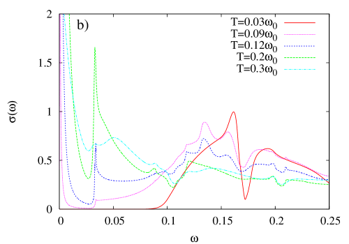
Figure 4: (Color online) Optical conductivity in the adiabatic regime $\gamma=0.1$, at an intermediate value of the coupling strength $\lambda=0.9$. a) the absorption is ”weak-coupling like” at low temperatures, with a clear threshold at $\omega=\omega_{0}$, and becomes ”strong-coupling like” at higher temperatures, causing a non-monotonic evolution of the spectral weight. b) a detailed view of the temperature evolution around the one-phonon threshold, where Polaron Interband Transitions appear.

V Polaron crossover in the adiabatic regime

The critical coupling strength for polaron formation was identified in Ref. xover as the value at which $dE_{0}/dg$ has maximum slope, which follows approximately $\lambda_{c}(\gamma)\simeq 0.84+0.9\gamma$ at small $\gamma$ (note that this derivative is related, through the Hellmann-Feynman theorem, to the electron-lattice correlation function). The width of the crossover region, obtained by looking at the maximum slope of $|\partial^{2}E_{0}/\partial g^{2}|$, is roughly given by $\Delta\lambda\simeq\gamma/2$ (cf. Fig. 3.b in ref xover , reported in Fig. 2 here), and vanishes in the adiabatic limit where the polaron formation becomes a true localization transition.

In this Section, we address the specific properties of the optical absorption in the adiabatic polaron crossover region. The present results extend the preliminary results obtained in Ref.BRoptcond allowing an inspection of the very low temperature regime, which turns out to be crucial to understand the evolution of the optical properties. We show that the adiabatic crossover region has two original signatures: The first is a coexistence of both weak and strong coupling characters in the optical conductivity, with a transfer of spectral weight between the two occurring at very low temperatures. The second is the emergence of narrow absorption features at low frequencies (of the order of, or even below the phonon frequency) with a non monotonic temperature dependence, corresponding to resonant transitions between long-lived states in the polaron excitation spectrum. We finally provide a semi-analytical expression for the optical conductivity in the zero temperature limit, that corrects Eq. (7) of Ref. BRoptcond .

V.1 Low temperature transfer of spectral weight

A typical optical conductivity spectrum in the crossover region is shown in Fig. 4.a, for $\gamma=0.1$ and $\lambda=0.9$. The data at the lowest temperature (red full curve) are very similar to the $\lambda=0.7$ results of Fig. 3.a, with a marked single-phonon edge at $\omega=\omega_{0}$ as given by Eq. (10), followed by a multi-phonon structured high frequency tail. Such “weak-coupling” behavior is in agreement with the fact that $\lambda=0.9$ lies slightly below the critical value $\lambda_{c}(\gamma=0.1)\simeq 0.93$. Upon increasing the temperature (green dashed curve), the optical absorption develops a broad maximum at high frequency typical of the polaronic regime, comparable to what is seen at $\lambda=1.1$ in Fig. 3.b. Remarkably, this occurs at temperatures much below the phonon quantum to thermal crossover at $T\sim\omega_{0}/2$, suggesting that such transfer of spectral weight is governed by an electronic energy scale.

To understand the origin of this phenomenon, a more detailed analysis of the single-particle spectral function is needed. As can be seen in Eq. (II), the calculation of the optical conductivity involves a convolution of the two quantities $\rho(\epsilon,\nu+\omega)$ and $e^{-\beta(\nu-E_{0})}\rho(\epsilon,\nu)$. Due to the exponential weighting factor, the contributions to $\rho(\epsilon,\nu)$ at $\nu>E_{0}$ are strongly suppressed at low temperatures, and only the states related to phonon emission processes at $\nu<E_{0}$ will contribute. For such incoherent states, the spectral function is directly proportional to the scattering rate $Im\Sigma(\nu)$ [cf. Eq. (49) in App. B]. Therefore, neglecting the $\epsilon$-dependence in Eq. (II), the optical spectrum is roughly proportional to a convolution of the spectral density $N^{*}(\nu+\omega)$ with the weighted scattering rate $e^{-\beta(\nu-E_{0})}Im\Sigma(\nu)$. Both of these quantities are illustrated in Fig. 5.

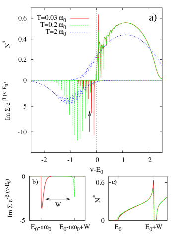
Figure 5: (Color online) a) Spectral density $N^{*}$ and weighted scattering rate $Im\Sigma(\nu)e^{-\beta(\nu-E_{0})}$ at $\lambda=0.9$ and $\gamma=0.1$, at different temperatures. b) Expanded view of a generic $n$-th peak in the weighted scattering rate ($n=3$, indicated by an arrow in the main panel, whose width equals the renormalized polaron bandwidth $W$ (the data at $T=0.03\omega_{0}$ have been multiplied by a factor $10^{3}$). The weight moves from the bottom to the top of the band at $T\sim W$. c) Expanded view of the polaron band in the spectral density $N^{*}$, separated from the high-energy continuum by a gap.

With the present choice of parameters, the spectral density at low temperature (upper panel of Fig. 5.a) consists of a single subband of width $W<\omega_{0}$ (the polaron band, expanded in Fig. 5.c) disconnected from the electron continuum at higher energy. Scattering processes are suppressed below $E_{0}+\omega_{0}$ because we are considering dispersionless optical phonons, so that the whole polaron band represents coherent long-lived states at low temperature. In contrast, higher energy states at $\nu>E_{0}+\omega_{0}$ are mostly incoherent, being strongly scattered by phonons. The marked asymmetry of the polaron band in Fig. 5.c comes from the fact that the band dispersion flattens in proximity of the band top, where the states have a more localized character. This coexistence of free-electron like states at low momenta and localized states at high momenta Fehske-momentum is crucial here, and can be understood from the following argument: In the weak coupling limit, the spectral density develops a dip at $\nu=E_{0}+\omega_{0}$ corresponding to the threshold for one-phonon scattering. Below this value, the band dispersion flattens due to the hybridization with the (dispersionless) phonon states, leading to a very large density of states. When $\lambda$ increases, the dip eventually becomes a true gap and a polaron band of width $W<\omega_{0}$ emerges from the continuum, retaining a characteristic asymmetric shape with a maximum close to the top edge.

The excitation spectrum hardly changes when going from $T=0.03\omega_{0}$ to $T=0.2\omega_{0}$, except for the appearance of few exponentially weak replicas of the polaron band at $\nu<E_{0}$ (see Figs. 5.a and 5.c). On the contrary, the weighted scattering rate (lower panel of Fig. 5.a) undergoes a drastic change in the same temperature range. At $T=0.03\omega_{0}$, the latter consists of a pattern of equally spaced peaks at $\nu=E_{0}-n\omega_{0}$, whose intensity decays as $\nu$ moves away from the ground state energy. Retaining only the (largest) peak at $E_{0}-\omega_{0}$, we see that the convolution integral ${\cal D}$ roughly follows the form of the spectral density $N^{*}(\omega+\omega_{0}-E_{0})$, with a gap below $\omega=\omega_{0}$ and a maximum around $\omega\approx E_{P}$. The behavior changes at $T=0.2\omega_{0}$, where the weighted scattering rate acquires a gaussian distribution centered at an energy $\sim E_{P}$ below the ground state, so that the maximum of ${\cal D}$ moves to $\omega\approx 2E_{P}$. Clearly, the transfer of spectral weight seen in Fig.4.a when going from $T=0.03\omega_{0}$ to $T=0.2\omega_{0}$ must be traced back to the change of behavior in the excitations at $\nu<E_{0}$ described here.

A more careful look at Fig. 5.a (expanded in Fig. 5.b) shows that the change in the overall distribution of $Im\Sigma e^{-\beta(\nu-E_{0})}$ is accompanied by a slight shift of the position of the individual peaks. In fact, as can be shown by direct inspection of the continued fraction expansion of Ref.depolarone , each peak at $\nu<E_{0}$ is a replica of the polaron band at $E_{0}$, of width $W$. At temperatures $T\ll W$, due to the exponential weighting factor, only the low momentum states close to the bottom edges contribute (cf. Fig. 5.b). Such states are free-electron like, and give rise to an optical absorption spectrum with a weak coupling character. As $T\gtrsim W$, on the other hand, more localized higher momentum states come into play, and the polaronic behavior is recovered. We remark that this “reentrant” behaviour is not restricted to the zero density case treated here. It can be found also in a two site cluster sim0ne as well as in the Holstein model at half filling centroide . The reason is ultimately due to the different roles played by the quantum and thermal fluctuations in the polaron crossover region. Quantum fluctuations are known to stabilize the non-polaronic phase, while incoherent fluctuations such as static disorder or thermal fluctuations stabilize the polaron. As the temperature increases, polarons are therefore first stabilized, before they eventually dissociate at a higher temperature.

According to the above arguments, the transfer of spectral weight illustrated in Fig. 4.a is ultimately controlled by a temperature scale set by the renormalized bandwidth $W$, whose evolution with the interaction strength is shown in Fig. 6. In the strong coupling regime, where $W$ vanishes exponentially, such phenomenon can hardly be observed in practice. On the other hand, the very existence of a polaron subband separated from the continuum of excited states requires moderately large values of $\lambda$, and the coexistence of electron-like states and localized states is specific to the adiabatic regime. The competition between all these conditions explains why the low-temperature transfer of spectral weight described here occurs in the vicinity of the adiabatic polaron crossover, roughly for $\lambda_{c}-0.5\gamma\lesssim\lambda\lesssim\lambda_{c}+\gamma$ and $\gamma\lesssim 0.5$ (shaded area in Fig.2).

A formal expression for the optical conductivity in the limit $T\ll W$ is derived in App. B, that we reproduce here:

$$\sigma(\omega) = [1-{\cal W}(0)]\frac{\pi}{\omega}\times$$

$$\times \frac{\sum_{p=1}^{\overline{p}}\int d\epsilon N(\epsilon)\phi(\epsilon)\rho^{>}(\epsilon,\omega+E_{0}-p\omega_{0})\overline{u}_{p}(\epsilon)}{\sum_{p=1}^{\infty}\int d\epsilon N(\epsilon)\overline{u}_{p}(\epsilon)}$$

where ${\cal W}(0)$ is a constant between $0$ and $1$ depending on the interaction parameters, and the functions $\overline{u}_{p}(\epsilon)$ are defined in Eq. (62). This formula replaces Eq. (7) of Ref. BRoptcond , which was incorrectly identified with the zero temperature limit of the optical absorption but is instead a preasymptotic contribution as $T\rightarrow 0$.

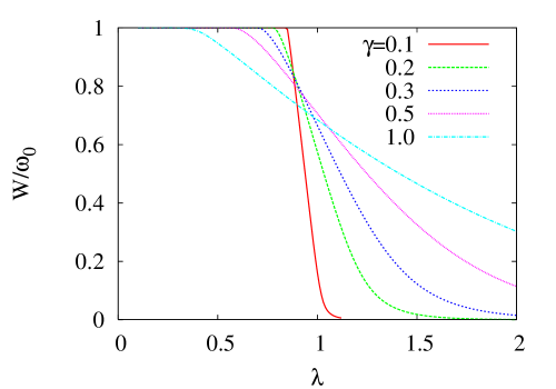
Figure 6: (Color online) Width of the polaron band as a function of the interaction parameter $\lambda$ for different values of the adiabaticity parameter $\gamma$, at $T=0$.

V.2 Polaron Interband Transitions

A detailed view of the low frequency optical absorption in the intermediate coupling regime is presented in Fig. 4.b. As was mentioned in the previous Section, the spectrum at the lowest temperature (full red curve) has a sharp threshold at $\omega=\omega_{0}$, followed by an absorption pattern which roughly reproduces the shape of the single particle spectral density, shifted by $\omega_{0}$ [see the weak coupling formula (25) in the appendix, as well as its generalization Eq. (V.1)]. For example, the peak at $\omega\simeq 0.17$ is directly related to the maximum observed in the spectral density at the top of the polaron band (compare Fig. 4.b with Fig. 5.c), and its position coincides with the expected value $\omega=\omega_{0}+W=0.173$. Upon increasing the temperature, the most striking effect in this low-frequency region is the emergence of a sharp asymmetric peak within the gap, whose intensity follows a puzzling non-monotonic temperature dependence. Such resonance has already been reported in Ref. BRoptcond , where it was termed polaron interband transition (PIT), and suggested as a possible explanation of the peaks experimentally observed in Ref.TAIR . In order to understand its origin, one has to go beyond the low-temperature arguments presented in the previous Section, and take into account the contributions to the convolution integral in Eq. (II) coming from the states at $\nu>E_{0}$.

Because of thermal activation, there is a non-vanishing probability for transitions involving an initial state at energies above the ground state. The Fermi golden rule tells us that the transition probability at a given frequency $\omega$ will be proportional to the conjugate density of the initial and final states separated by $\omega$, times the occupation factor of the initial state. Therefore, a sharp resonance will arise if: i) many pairs of initial and final states exist that are separated by approximately the same energy $\omega^{*}$, which is equivalent to the condition that the energy dispersions in the initial and final subband are parallel; ii) such states are long lived, which is possible at low temperatures because $Im\Sigma$ is exponentially suppressed in the whole region $E_{0}<\nu<E_{0}+\omega_{0}$. Both conditions can be fulfilled in the intermediate coupling regime, as illustrated in Fig. 3 of Ref. BRoptcond . Upon increasing the temperature, the states involved in the transitions are eventually smeared out by thermal disorder, which explains the non monotonic temperature dependence of this resonance.

This qualitative argument can be formalized as follows (the detailed calculations are presented in Appendix B). When the scattering rate in the initial state is negligible, the spectral function $\rho(\epsilon,\nu)$ can be replaced by a delta function and the convolution integral in Eq. (II) becomes [cf. Eq. (41)]:

$${\cal D}(\omega) \simeq \int_{E_{0}}^{\infty}d\nu N(\nu-Re\Sigma(\nu))\phi(\nu-Re\Sigma(\nu))e^{-\beta(\nu-E_{0})}$$ (15)

$$\times \left(-\frac{1}{\pi}Im\frac{1}{\omega+Re\Sigma(\nu)-Re\Sigma(\nu+\omega)+i\Gamma}\right).$$

This quantity is maximum for those values of $\omega$ such that there is a wide range of energies $\nu$ where the denominator is close to zero. This condition corresponds to the pair of equations

$$\omega+Re\Sigma(\nu)-Re\Sigma(\nu+\omega)=0$$

$$\left.\frac{\partial Re\Sigma}{\partial\nu}\right|_{\nu}-\left.\frac{\partial Re\Sigma}{\partial\nu}\right|_{\nu+\omega}=0$$ (16)

whose solution we denote as $\omega^{*}$ and $\nu^{*}$. The optical conductivity can be evaluated by expanding Eq. (15) around these special values, and taking $\Gamma\equiv-Im\Sigma(\nu+\omega)$ to be small and constant in the frequency range of interest, which gives

$$\sigma_{PIT}(\omega)\simeq\frac{\pi}{{\sqrt{2Q\Gamma}\omega}}\frac{(1-e^{-\beta\omega})e^{-\beta\nu^{*}}}{{\cal N}(\beta)}\times$$ (17)

$$\times N(\nu^{*}-Re\Sigma(\nu^{*}))\phi(\nu^{*}-Re\Sigma(\nu^{*})){\cal F}[\frac{M(\omega-\omega^{*})}{\Gamma}].$$

where $M$ is the effective mass of the initial (and final) states and $Q$ is related to the curvature of the dispersion. The function

$${\cal F}(y)=\frac{\sqrt{y+\sqrt{y^{2}+1}}}{\sqrt{y^{2}+1}}$$ (18)

has an inverse square root tail $\sim y^{-1/2}$ at large $y$, and tends to $1$ for $0<y\lesssim 1$, giving rise to a narrow peak of width $\Delta\omega\sim\Gamma/M$. Such asymmetric shape can be clearly identified in Fig.4.b, at $\omega^{*}\simeq 0.3\omega_{0}$. Reminding that $\Gamma\sim e^{-\beta\omega_{0}}$, and using the definition Eq. (4), we see that the weight of the narrow peak scales as

$$w(\beta)\sim\frac{1-e^{-\beta\omega^{*}}}{\omega^{*}}\frac{e^{-\beta(\nu^{*}-E_{0}+\omega_{0}/2)}}{{\cal N}(\beta)}.$$ (19)

This quantity rises exponentially with temperature and then decreases as a power law at temperatures above some fraction of $\omega_{0}$, whose precise value depends on the parameters $\omega^{*}$, $\nu^{*}$ and $W$.

VI Conclusion

In this work, we have studied the optical absorption of electrons interacting with phonons in the framework of the Holstein model, applying a unified treatment — the dynamical mean-field theory — which is able to account for both the quantum nature of the phonons and the effects of a finite electronic bandwidth. The present non-perturbative approach allows to span all the ranges of parameters of the model, from weak to strong electron-phonon interactions, and from the adiabatic to the antiadiabatic limit. The limits of validity of the standard available formulas are pointed out, and the quantitative and qualitative deviations arising in wide ranges of the parameters space are analyzed, which will hopefully lead to a better understanding of the experiments performed on polaronic systems.

In the antiadiabatic regime, the present method allows to address the evolution of the optical absorption away from the single molecule limit, where the spectra reduce to a distribution of delta functions. Considering a finite bandwidth $D$ yields an intrinsic width to the multi-phonon peaks, which is not uniform over the whole spectral range (peaks at high frequency are broader than at low frequency) and generally does not obey the exponential narrowing predicted by the standard approaches. Moreover, in the strong coupling regime, the peaks are found to broaden upon increasing the temperature, in marked contradiction to the commonly accepted results in the literature, which are based on uncontrolled approximations.

The situation is different in the adiabatic regime, where it is found that the nature of the optical absorption changes drastically at the sharp polaron crossover occurring at $\lambda\simeq\lambda_{c}$. The weak coupling formula (10) is shown to extend qualitatively to finite values of $\lambda$, up to the polaron crossover, whose proximity is signaled by the emergence of a fine structure related to multi-phonon processes. Beyond the polaron crossover, the absorption mechanism in the strong coupling regime is found to depend on an additional parameter, the ratio $s/D$ between the broadening of the Franck-Condon line and the free-electron bandwidth. The usual polaronic gaussian lineshape described by Eq. (12) is recovered for $s\gg D$. In the opposite limit, $s\ll D$, a different absorption mechanism sets in, related to the photoionization of the polaron towards the free-electron continuum. Correspondingly, the lineshape in this limit is entirely determined by the shape of the free-electron band, and is characterized by a sharp absorption edge at finite frequency, as described by Eq. (13). The optical spectra at intermediate values of $s/D$, a situation often encountered in real systems, are not properly described by any of the two limiting formulas Eqs. (12) and (13). In particular, due to finite bandwidth effects, the frequency of the absorption maximum is appreciably lower than the usual estimate $\omega_{max}=2E_{P}$, and the lineshape is more asymmetric than the gaussian of Eq. (12), which should be taken into account when interpreting experimental data.

In the intermediate coupling region around $\lambda\simeq\lambda_{c}$, qualitatively new features arise that are distinctive of the adiabatic polaron crossover. First, the optical absorption exhibits a reentrant behavior, switching from weak-coupling like to polaronic-like upon increasing the temperature. The temperature scale that governs such transfer of spectral weight is of electronic origin, being set by the renormalized polaronic bandwidth $W$, a quantity that is necessarily less (or equal) than the phonon energy, and rapidly decreases upon increasing $\lambda$. In addition, sharp peaks with a non-monotonic temperature dependence emerge at typical phonon energies, and are most clearly visible in the region below the single-phonon absorption gap. These can be ascribed to thermally excited resonant transitions between long lived states located in different subbands in the polaron internal structure, and their peculiar temperature dependence results from the competition between the thermal activation and the thermal broadening of the corresponding states.

To conclude, let us observe that the present formalism can in principle be applied to any finite-dimensional lattice by replacing $N(\epsilon)$ of Eq. (7) with the appropriate DOS. It has already been mentioned (cf. end of Section V A) that Eq. (13) reproduces very accurately the one-dimensional exact diagonalization data of Ref. ray obtained for $s\ll D$. Even away from this limit, however, preliminary DMFT results obtained using the one-dimensional DOS $N(\epsilon)=1/(\pi\sqrt{D^{2}-\epsilon^{2}})$ are in qualitative agreement with the numerical results of Ref. Fehske-opt , at least in the high frequency part of the spectra. In particular, in the intermediate coupling regime, the polaronic absorption maximum appears to be shifted downwards as compared with the three-dimensional case (cf. Figs. 4 and 6 in Ref. Fehske-opt ). This result can be understood from the arguments presented in Section V A by observing that due to the singularity of the one-dimensional DOS, the function $N^{*}$ appearing in Fig. 5 is peaked around $\nu-E_{0}\simeq 0$ instead of $\nu-E_{0}\simeq E_{P}$.

Concerning vertex corrections, which are absent in our formalism, we have seen that these are irrelevant in the limiting regimes of weak and strong coupling, as well as in the adiabatic regime $s\ll D$ at any coupling strength and for any lattice dimensionality (including in one dimension). On the other hand, their presence could quantitatively change the optical spectra when both the phonon frequency and coupling strength lie in the intermediate regime. From this point of view, the polaron interband transitions evidenced in the intermediate adiabatic crossover region, relying on the resonance condition Eq. (16), could indeed be affected by the inclusion of vertex corrections.

As a last remark, we stress that the description of the optical properties provided in this work, based on the solution of the Holstein model for a single particle, is valid in principle for a system of independent polarons. How the above features are modified by polaron-polaron interactions at finite densities remains a fundamental question, that needs to be addressed in the future.

Appendix A: Derivation of limiting formulas

Weak coupling limit, low temperatures $T\ll\omega_{0}$.

In the limit of weak interactions, we can write the spectral function $\rho_{\epsilon}$ appearing in Eq. (II) as

$$\rho_{\epsilon}=\rho^{(0)}_{\epsilon}+\delta\rho_{\epsilon}$$

where $\rho^{(0)}_{\epsilon}$ is non-interacting and reduces to a delta function. Substituting the previous expression in Eq. (II) and taking into account only the contributions proportional to $\delta\rho$ we get

$${\cal D}(\omega) = \int d\epsilon N(\epsilon)\phi(\epsilon)\int d\nu e^{-\beta(\nu-E_{0})}\times$$

$$\times \left[\rho^{(0)}_{\epsilon}(\nu)\delta\rho_{\epsilon}(\nu+\omega)+\delta\rho_{\epsilon}(\nu)\rho^{(0)}_{\epsilon}(\nu+\omega)\right]$$

Performing the two integrals in $\nu$ yields

$${\cal D}(\omega) = -\frac{1}{\pi\omega^{2}}\int d\epsilon N(\epsilon)\phi(\epsilon)\left[e^{-\beta(\epsilon-E_{0})}Im\Sigma(\epsilon+\omega)+\right.$$ (21)

$$\left.Im\Sigma(\epsilon-\omega)e^{-\beta(\epsilon-\omega-E_{0})}\right]$$

Perturbation theory gives, to order $g^{2}$ and at zero density

$$\Sigma(\omega)=g^{2}\left[(1-n_{B})G(\omega-\omega_{0})+n_{B}G(\omega+\omega_{0})\right]$$ (22)

where $n_{B}$ is the Bose occupation number. Substituting the self-energy into Eq. (21) gives rise to 4 terms, namely:

$${\cal D}(\omega) = \frac{g^{2}}{\omega^{2}}\int d\epsilon N(\epsilon)\phi(\epsilon)\times$$ (23a)

$$\times \left[(1-n_{B})e^{-\beta(\epsilon-E_{0})}N(\epsilon+\omega-\omega_{0})\right.$$

$$+ n_{B}e^{-\beta(\epsilon-E_{0})}N(\epsilon+\omega+\omega_{0})$$ (23b)

$$+ (1-n_{B})e^{-\beta(\epsilon-\omega-E_{0})}N(\epsilon-\omega-\omega_{0})$$ (23c)

$$+ n_{B}e^{-\beta(\epsilon-\omega-E_{0})}N(\epsilon-\omega+\omega_{0})\left.\right]$$ (23d)

At temperatures $T\ll\omega_{0}$, the second and third term are exponentially small, and can be neglected. Note also that, since the above terms are explicitely proportional to $g^{2}$, the normalization factor (6) can be evaluated in the non-interacting limit, which gives $\mathcal{N}(\beta)=(2/\beta)e^{-\beta D}I_{1}(\beta D)$, where $I_{1}$ is the modified Bessel function of the first kind, whose limiting behaviors are $\mathcal{N}\simeq\sqrt{2/\pi}/(\beta D)^{3/2}$ for $\beta D\gg 1$ and $\mathcal{N}\to 1$ for $\beta D\ll 1$.

At temperatures much smaller than the width of the band under study, due to the presence of the exponential factors, only the low energy edges of the density of states (corresponding to low-momentum states) contribute to the integrals in Eq. (23). In this case we can make use of the following approximation:

$$\int_{\nu}d\epsilon e^{-\beta(\epsilon-\nu)}(\epsilon-\nu)^{\ell}f(\epsilon)\simeq\frac{f(\nu)}{\beta^{\ell+1}}\Gamma(\ell+1)$$ (24)

where $\Gamma(n)$ is the Euler gamma function and $f(\nu)$ is a generic continuous function. By substituting the previous expression in equations (23), only the term (23d) survives in the limit $T\ll D$, and we obtain

$$\left.\sigma(\omega)\right|_{T\ll D}=\frac{g^{2}\pi}{\omega^{3}}\phi(\omega-D-\omega_{0})N(\omega-D-\omega_{0}).$$ (25)

which corresponds to a sharp edge behavior $\sigma(\omega)\sim(\omega_{0}-\omega)^{3/2}$, in agreement with perturbative calculations in three dimensionsMahan . Similar arguments lead to $\sigma(\omega)\sim(\omega_{0}-\omega)^{d/2}$ if one assumes the appropriate $d-$dimensional noninteracting band in Eq. (II).

In the adiabatic regime, the condition $T\ll\omega_{0}$ ensures that $T\ll D$. In the opposite antiadiabatic regime, the result (25) remains valid for $T\ll D$, while for $D\ll T\ll\omega_{0}$, we can set the exponential factors equal to $1$ in Eqs. (23), leading to

$$\left.\sigma(\omega)\right|_{D\ll T\ll\omega_{0}}=\frac{g^{2}\pi}{\omega^{3}}F(\omega-\omega_{0})$$ (26)

where the function $F$ is defined as

$$F(y)=\int_{-D}^{D-|y|}dxN(x)N(x+|y|)[\phi(x)+\phi(x+|y|)]$$ (27)

(note that current vertex corrections are not included in this formula; however, they lead to the same functional form in both the adiabatic and anti-adiabatic limits). In this temperature range, the absorption related to the excitation of a single phonon is nonzero in the range $\omega_{0}-2D<\omega<\omega+2D$ and is symmetric around $\omega=\omega_{0}$ (see the inset in Fig. 1.a) where $\sigma=(128/45\pi)g^{2}D/\omega_{0}^{3}$. By comparing Eq. (27) with Eq. (25), we see that in the antiadiabatic regime, the absorption peak is shifted to lower frequency when the temperature is increased above $T\simeq D$, and the sharp square root edge is converted into $\sigma(\omega)\sim[\omega-(\omega_{0}-2D)]^{3}$.

Strong coupling limit, narrow bands.

In the adiabatic limit ($\omega_{0}\to 0$), the strong coupling regime can be attained by increasing $\lambda$ while keeping the polaron energy $E_{P}$ finite. In this case, the spectral function of a single polaron becomes independent of momentum (the $\epsilon$ index drops because the bandwidth $D=E_{P}/\lambda\to 0$). The self-energy in Eq. (2) becomes $\Sigma=-gX$, where $X$ is a classical variable that acts as a source of disorder that modifies the electronic levels according to the Boltzmann distribution depolarone ; HoHu . Correspondingly, the spectral function tends to a gaussian

$$\rho(\nu)=\frac{1}{\sqrt{2\pi s^{2}}}\exp\left[-\frac{\nu^{2}}{2s^{2}}\right]$$ (28)

whose variance $s=\sqrt{2E_{P}T}$ is determined by the thermal fluctuations of the classical phonon field. Once the $\epsilon$-integral is factored out (yielding a numerical prefactor), the convolution integral in Eq. (II) is readily evaluated and yields

$$\sigma(\omega)_{s\gg D}=\frac{\pi D^{2}}{4\omega}\frac{1-e^{-\beta\omega}}{\sqrt{4\pi s^{2}}}\exp\left[-\frac{(\omega-2E_{P})^{2}}{4s^{2}}\right]$$ (29)

which coincides with the standard result of Refs. old ; Reik ; Mahan ; Emin93 It should be noted that, due to the initial assumption $\omega_{0}=0$, the above derivation is strictly valid only in the high temperature limit $T\gg\omega_{0}$. However, Eq. (29) can be generalized to all temperatures by setting

$$s^{2}(T)=E_{P}\omega_{0}\coth(\frac{\omega_{0}}{2T})$$ (30)

[note that Eq. (28) is also valid at $T=0$, in which case the variance is determined by the phonon zero point fluctuations and becomes $s=\sqrt{E_{P}\omega_{0}}$ depolarone ; HoHu ]. Eq. (29) is valid in the strong coupling adiabatic regime provided that $s\gg D$.

Note that in the limit of an isolated molecule ($D=0$) at finite $\omega_{0}$, which is qualitatively representative of the antiadiabatic regime, the spectral function consists of a distribution of delta functions, describing the multi-phonon excitations inside the polaron potential-wellMahan . The convolution integral in Eq. (II) can be carried out, and yields a discrete absorption spectrum, whose envelope in the strong coupling limit $\alpha^{2}=E_{P}/\omega_{0}\gg 1$ coincides with Eq. (29).

Strong coupling limit, wide bands.

There is an alternative way of reaching the polaronic adiabatic regime, i.e. assuming that the phonon induced broadening of electronic levels $s$ is negligible compared to the electron dispersion $D$. For sufficiently large $E_{P}$, the optical absorption will be due to transitions from a perfectly localized level whose electronic energy is $-2E_{P}$, to the free-electron continuum. Put in the context of the convolution integral Eq. (II), this corresponds to the following replacements

$$\rho(\epsilon,\omega+\nu) = \delta(\epsilon-\omega-\nu)$$ (31)

$$\rho(\epsilon,\nu) = \delta(\nu+2E_{P})$$ (32)

where the last quantity is independent of $\epsilon$. The result is

$$\sigma(\omega)_{s\ll D\ll E_{P}}=\pi\frac{1-e^{-\beta\omega}}{\omega}\phi(\omega-2E_{P})N(\omega-2E_{P})$$ (33)

This result is equivalent to that reported in Ref. ray ; Firsov for small polarons in one-dimensional systems, and in Ref. Emin93 for large polarons in two and three dimensions. However, the limit of a perfectly localized state assumed here is strictly valid only for $E_{P}\to\infty$. At finite $E_{P}$, a more accurate formula can be obtained by restoring the $\epsilon$-dependence of the initial state in Eq.(32). This can be achieved by taking

$$\rho(\epsilon,\nu)=-\frac{1}{\pi}Im\frac{1}{\nu-\Sigma(\nu)-\epsilon}\simeq-\frac{1}{\pi}\frac{Im\Sigma(\nu)}{(\nu-\epsilon)^{2}}$$ (34)

where we have used the fact that both $Re\Sigma$ and $Im\Sigma$ are small around $\nu\simeq-2E_{P}$. The scattering rate at these energies can in principle be extracted from the atomic limit of Ref. Mahan , because it is a local quantity. For $s\to 0$ it is given by:

$$-\frac{1}{\pi}Im\Sigma(\nu)e^{-\beta(\nu+E_{P})}=\nu^{2}\delta(\nu+2E_{P})$$ (35)

Evaluation of Eq. (II) now yields a more asymmetric shape

$$\sigma(\omega)_{s\ll D}=\pi\frac{4E_{P}^{2}}{\omega^{2}}\frac{1-e^{-\beta\omega}}{\omega}\phi(\omega-2E_{P})N(\omega-2E_{P})$$ (36)

which reduces to the previous Eq. (33) in the limit $E_{P}\gg D$.

It should be noted that when the appropriate one-dimensional DOS is used, Eq. (36) describes much better the exact diagonalization data of Ref. ray than Eq. (33) itself, that was used by Alexandrov and coworkers in their Figs. 3.c and 3.d. A possible generalization of the present scheme to finite values of $s$ is currently under study.prepa

Appendix B: Optical conductivity at low temperature

In this appendix we give a formal expression for the optical conductivity in the limit of low temperatures, which is useful for the understanding of the results in the intermediate coupling regime.

We can formally separate $\rho(\epsilon,\nu)$ in two parts, at energies above and below the ground state

$$\rho(\epsilon,\nu)=\theta(\nu-E_{0})\rho^{>}(\epsilon,\nu)+\theta(E_{0}-\nu)\rho^{<}(\epsilon,\nu)$$ (37)

[a similar separation will hold for $N^{*}(\nu)$] Accordingly, in Eq. (4) we can separate in both numerator $\cal{D}$ and denominator $\cal{N}$ the contributions coming from energies lower and higher than the ground state energy $E_{0}$, obtaining

$${\cal D}(\omega) = {\cal D}^{>>}(\omega)+{\cal D}^{<>}(\omega)+{\cal D}^{<<}(\omega)$$ (38)

$${\cal N} = {\cal N}^{>}+{\cal N}^{<}$$ (39)

In Eq. (38) the last contribution is negligible at low temperature for $\omega>0$ since $\rho^{<}(\omega+\nu)$ decays exponentially as $\exp[-\beta(E_{0}+\omega-\nu)]$. On the contrary both ${\cal N}^{<}$ and ${\cal D}^{<>}(\omega)$ cannot be neglected due to the thermal population factor $\exp[-\beta(\nu-E_{0})]$ appearing in Eq. (4). Let us calculate the remaining four terms separately.

Calculation of ${\cal D}^{>>}(\omega)$

$${\cal D}^{>>}(\omega) = \int_{E_{0}}^{\infty}d\nu\int_{-D}^{D}d\epsilon N(\epsilon)\phi(\epsilon)e^{-\beta(\nu-E_{0})}\times$$ (40)

$$\times \rho^{>}(\epsilon,\nu)\rho^{>}(\epsilon,\omega+\nu)$$

At low temperature, $\rho^{>}(\epsilon,\nu)$ weighted by the exponential factor gets contributions only for $\nu\simeq E_{0}$. This occurs when the temperature is so low that both the thermal occupations of the first excited subband and of the incoherent background edge at $\nu=E_{0}+\omega_{0}$ are negligible, i.e. for $\beta\omega_{0}\gg 1$. In this case the scattering rate is negligible (the low-energy states are coherent), $\rho^{>}(\epsilon,\nu)$ can be replaced by $\delta[\nu-\epsilon-Re\Sigma(\nu)]$ and the integral in $\epsilon$ appearing in Eq. (40) can be carried out:

$${\cal D}^{>>}(\omega) = \int_{E_{0}}^{\infty}d\nu N(\nu-Re\Sigma(\nu))\phi(\nu-Re\Sigma(\nu))$$ (41)

$$\times e^{-\beta(\nu-E_{0})}\rho^{>}(\nu-Re\Sigma(\nu),\omega+\nu).$$

At temperatures lower than the renormalized bandwidth $W$, the thermal weighting factor selects an integration range of width $T$ around the ground state energy where, from Eqs. (7) and (8), we have

$$N(\nu-Re\Sigma(\nu)) \simeq \frac{2}{\pi D^{2}}\sqrt{2D/Z}(\nu-E_{0})^{1/2}$$ (42)

$$\phi(\nu-Re\Sigma(\nu)) \simeq \frac{2D/Z}{3}(\nu-E_{0})$$ (43)

Here $Z=(1-\partial_{\nu}Re\Sigma)^{-1}$ is the ground state quasiparticle residue, equal to the inverse of the effective mass in the case of a purely local self-energy. Making use of Eq. (24) and the definition $E_{0}-Re\Sigma(E_{0})=-D$, we obtain

$${\cal D}^{>>}(\omega)=C(T)\left(-\frac{1}{\pi}Im\frac{1}{\omega+E_{0}+D-\Sigma(\omega+E_{0})}\right)$$ (44)

with $C(T)=\sqrt{2/\pi}\ D^{2}/Z^{3/2}\ (T/D)^{5/2}$ for $T\ll W$. In the strong coupling regime, the polaron band becomes extremely narrow and can itself be replaced by a delta function. For $T\gg W\to 0$, we obtain the same expression Eq. (44) with $C(T)\simeq 4W^{2}\to 0$, and this contribution becomes negligible.

Polaron interband transitions

The previous formula for ${\cal D}^{>>}$ was derived assuming that $T\ll\omega_{0}$. Upon increasing the temperature, other contributions arise that involve states at frequencies $\nu$ away from the ground state $E_{0}$. These can give rise to sharp resonances in the optical absorption spectra (see Section IV B). Eq. (41) can be rewritten as

$${\cal D}^{>>}(\omega)=\int_{E_{0}}^{\infty}d\nu N(\nu-Re\Sigma(\nu))\phi(\nu-Re\Sigma(\nu))$$

$$\times e^{-\beta(\nu-E_{0})}\left(-\frac{1}{\pi}Im\frac{1}{\omega+Re\Sigma(\nu)-Re\Sigma(\nu+\omega)+i\Gamma}\right)$$

where $\Gamma=-Im\Sigma(\nu+\omega)$ is taken to be small and constant in the frequency range of interest. A resonance will arise for those values of $\omega$ such that there is a wide range of energies $\nu$ where the denominator is close to zero. This condition corresponds to the pair of equations

$$\omega+Re\Sigma(\nu)-Re\Sigma(\nu+\omega)=0$$

$$\left.\frac{\partial Re\Sigma}{\partial\nu}\right|_{\nu}-\left.\frac{\partial Re\Sigma}{\partial\nu}\right|_{\nu+\omega}=0$$

whose solutions we denote $\omega^{*}$ and $\nu^{*}$. Now the denominator in Eq. (Polaron interband transitions) can be expanded around these special points, which gives

$$M(\omega-\omega^{*})-Q(\nu-\nu^{*})^{2}+i\Gamma$$

$M=1-(\partial\Sigma/\partial\nu)_{\nu^{*}}$ being the (equal) effective mass of the initial (and final) states and $Q$ a parameter related to the curvature of $Re\Sigma$. If one assumes that the prefactors $N$ and $\phi$ are smooth functions in the vicinity of $\nu^{*}$, these can be taken out of the integral, which can be evaluated to

$${\cal D}^{PIT} \simeq \frac{N(\nu^{*}-Re\Sigma(\nu^{*}))\phi(\nu^{*}-Re\Sigma(\nu^{*}))}{\sqrt{2Q\Gamma}}$$ (46)

$$\times e^{-\beta\nu^{*}}{\cal F}[M(\omega-\omega^{*})/\Gamma]$$

where the function

$${\cal F}(y)=\frac{\sqrt{y+\sqrt{y^{2}+1}}}{\sqrt{y^{2}+1}}$$ (47)

tends to $1$ for $0<y\ll 1$ and has an inverse square root tail $\sim y^{-1/2}$ at large $y$.

Calculation of ${\cal D}^{<>}(\omega)$

$${\cal D}^{<>}(\omega) = \int_{E_{0}-\omega}^{E_{0}}d\nu\int_{-D}^{D}d\epsilon N(\epsilon)\phi(\epsilon)e^{-\beta(\nu-E_{0})}\times$$ (48)

$$\times \rho^{<}(\epsilon,\nu)\rho^{>}(\epsilon,\omega+\nu)$$

The excitations in $\rho^{<}$ are mostly incoherent, being due to the presence of thermally activated phonons. This is best expressed by showing explicitely the proportionality to the scattering rate

$$\rho^{<}(\epsilon,\nu)=-\frac{1}{\pi}\frac{Im\Sigma(\nu)}{(\nu-Re\Sigma(\nu)-\epsilon)^{2}+(Im\Sigma(\nu))^{2}}$$ (49)

Through Eq. (49), the product $e^{-\beta(\nu-E_{0})}Im\Sigma(\nu)$ appears in Eq. (48). A sample plot of this product is reported in Fig. 5.b. At energies below the ground state, taking advantage of the continued fraction expansion of Ref.depolarone , the imaginary part of $\Sigma$ can be approximately written as a sum of separate contributions

$$-Im\Sigma(\nu)=\sum_{p=1}^{\infty}e^{-\beta p\omega_{0}}u_{p}(\nu)$$ (50)

As was the case for ${\cal D}^{>>}$, we treat separately the cases $T\ll W$ and $T\gg W\to 0$. In the former case, $u_{p}$ is a function with a square root edge at $\nu=E_{0}-p\omega_{0}$

$$u_{p}(\nu)=\overline{u}_{p}\ (\nu-E_{0}+p\omega_{0})^{1/2}$$ (51)

which is reminiscent of the behaviour of the spectral density at energy $E_{0}-(p-1)\omega_{0}$ and $\overline{u}_{p}$ is an unknown weighting factor. As can be seen from Fig. 5.b, each $u_{p}(\nu)$ has a bandwidth which is independent on $p$, and equal to the width $W$ of the first polaronic band. Therefore, when $T\ll W$, the square root edges can all be replaced by delta functions by making use of Eq. (24). When Eqs. (50,51) are substituted in Eq. (48) the $\nu$-integral can be carried out, leading to

$${\cal D}^{<>}(\omega) = \Gamma(3/2)T^{3/2}\sum_{p=1}^{\overline{p}}\int_{-D}^{D}d\epsilon N(\epsilon)\phi(\epsilon)\times$$ (52)

$$\times \rho^{>}(\epsilon,\omega+E_{0}-p\omega_{0})\times$$

$$\times \frac{1}{\pi}\frac{\overline{u}_{p}}{(E_{0}-p\omega_{0}-\epsilon-Re\Sigma(E_{0}-p\omega_{0}))^{2}}$$

where $\overline{p}=int(\omega/\omega_{0})$. In Eq. (52) we have neglected the exponentially vanishing scattering rate $Im\Sigma$ in the denominator of Eq. (49). At higher temperatures, or in the strong coupling regime, where $\omega_{0}\gg T\gg W\to 0$, we can take

$$u_{p}(\nu)=\bar{u}_{p}^{\prime}\delta(\nu-E_{0}-W+p\omega_{0})$$ (53)

which leads to an expression analogous to Eq. (52), with the prefactor replaced by $e^{-\beta W}$ and $E_{0}\to E_{0}+W$, reflecting the fact that the dominant weight is now carried by localized excitations at the top of the band (see the discussion in Sec. III A).

Calculation of ${\cal N}^{>}$.

$${\cal N}^{>}=\int_{E_{0}}^{\infty}d\nu\int_{-D}^{D}d\epsilon N(\epsilon)e^{-\beta(\nu-E_{0})}\rho^{>}(\epsilon,\nu).$$ (54)

Since a gap of width $\omega_{0}$ separates the coherent pole of $\rho^{>}$ from the incoherent continuum, for $\beta\omega_{0}\gg 1$ only the lowest energy edge of the spectral density contributes to the integral Eq. (54). Using Eqs. (24,42) we get

$${\cal N}^{>}=\frac{2}{\pi D^{2}}\sqrt{2D/Z}\Gamma(3/2)T^{3/2}$$ (55)

Calculation of ${\cal N}^{<}$.

$${\cal N}^{<}=\int_{-\infty}^{E_{0}}d\nu\int_{-D}^{D}d\epsilon N(\epsilon)\rho^{<}(\epsilon,\nu).$$ (56)

As was stated before, $\rho^{<}$ represents incoherent states as given by Eq. (50). For $\beta W\gg 1$, the integrals in $\nu$ can be carried out with the help of Eq. (24) giving

$${\cal N}^{<} = \Gamma(3/2)T^{3/2}\sum_{p=1}^{\infty}\int_{-D}^{D}d\epsilon N(\epsilon)\times$$ (57)

$$\times \frac{1}{\pi}\frac{\overline{u}_{p}}{(E_{0}-p\omega_{0}-\epsilon-Re\Sigma(E_{0}-p\omega_{0}))^{2}}$$

At higher temperatures, $T\gg W$, we get an analogous result, with the prefactor replaced by $e^{-\beta W}$ and $E_{0}\to E_{0}+W$. By comparing the two expressions, it can be deduced that the term ${\cal N}^{<}$ changes behavior from $\sim T^{3/2}$ to $e^{-\beta W}$ at a temperature $T_{W}\sim W/\log(D/W)$. The resulting normalization factor ${\cal N}$ has the form $\sim T^{3/2}$ in the weak coupling regime and $\sim e^{-\beta W}\to 1$ in the strong coupling regime. In the intermediate coupling regime, where $W$ is of the order of $\omega_{0}$, a crossover between the two behaviors occurs at $T_{W}$.

Final formula for $\sigma(\omega)$ at $T=0$.

Collecting the results Eqs. (44,52,55,57) into Eq. (4) we get the final result. To separate the terms (44) and (55) which involve the coherent states close to the ground state $E_{0}$ from the remainder, it is useful to introduce a temperature dependent weight

$${\cal W}(T)=\frac{{\cal N}^{>}}{{\cal N}}$$ (58)

which tends to a constant for $T\ll W$, and to a (different) constant for $T\gg T_{W}$. Then

$$\sigma(\omega)={\cal W}(T)\sigma_{0}(\omega)+\left[1-{\cal W}(T)\right]\sigma_{1}(\omega)$$ (59)

where, from Eqs. (44,55):

$$\sigma_{0}(\omega)=\frac{\pi D/Z}{\omega}T\left(-\frac{1}{\pi}Im\frac{1}{\omega+E_{0}+D-\Sigma(E_{0}+\omega)}\right)$$ (60)

Eq. (60) is Eq. (7) of Ref. BRoptcond , where it was incorrectly identified with the zero temperature limit of the optical absorption (note that the linear dependence on temperature makes this contribution vanish at $T=0$).

Under the above hypothesis the remaining term $\sigma_{1}$ does not depend explicitely on temperature. In fact, using Eqs. (52,57) we get a formal expression

$$\sigma_{1}(\omega)=\frac{\pi}{\omega}\frac{\sum_{p=1}^{\overline{p}}\int d\epsilon N(\epsilon)\phi(\epsilon)\rho^{>}(\epsilon,\omega+E_{0}-p\omega_{0})\overline{u}_{p}(\epsilon)}{\sum_{p=1}^{\infty}\int d\epsilon N(\epsilon)\overline{u}_{p}(\epsilon)}$$ (61)

where

$$\overline{u}_{p}(\epsilon)=\frac{\overline{u}_{p}}{(E_{0}-p\omega_{0}-\epsilon-Re\Sigma(E_{0}-p\omega_{0}))^{2}}$$ (62)

and at $T=0$ we have $\sigma(\omega)=[1-{\cal W}(0)]\sigma_{1}(\omega)$. Note that, since the sum is limited to $\bar{p}$, at low temperature only the first term in the numerator of Eq. (61) contributes to the Drude peak at $\omega\simeq 0$ and to the one-phonon threshold at $\omega=\omega_{0}$ .

To recover the perturbative expression Eq. (25) we consider only a single contribution in the sums appearing in Eq. (61). Then we perform the integral in the numerator of Eq. (61) using the free spectral function $\rho^{>}(\epsilon,\omega+E_{0}-p\omega_{0})=\delta(\omega+E_{0}-p\omega_{0}-\epsilon)$ obtaining

$$\sigma_{1}(\omega)=\frac{\pi}{\omega}\frac{N(\omega+E_{0}-\omega_{0})\phi(\omega+E_{0}-\omega_{0})\overline{u}_{1}(\omega+E_{0}-\omega_{0})}{\int d\epsilon N(\epsilon)\overline{u}_{1}(\epsilon)}.$$ (63)

To proceed further we have from Eq. (22)

$$\overline{u}_{1}(\omega+E_{0}-\omega_{0})\simeq-2g^{2}\frac{2\sqrt{2D}}{D^{2}\omega^{2}}$$ (64)

where we have neglected the self-energy term in the denominator of $\overline{u}_{1}$ for $\beta\omega_{0}\gg 1$. Eq. (25) follows by multiplying (63) by the factor $(1-{\cal W})$.

References

- (1) I.G. Austin and N. F. Mott, Adv. Phys. 18, 41 (1969)
- (2) T. Holstein Ann.Phys. 8, 325 (1959), ibid. 343 (1959).
- (3) S. Fratini and S. Ciuchi, Phys. Rev. Lett. 91, 256403 (2003)
- (4) A.S. Alexandrov and J. Ranninger, Phys. Rev. B 45, R13109 (1992); J. Ranninger Phys. Rev. B 48, R13166 (1993)
- (5) G.D. Mahan, Many-Particle Physics, Plenum Press, New York, 2nd edition (1990)
- (6) H. Sumi, J. Phys. Soc. Jpn. 36, 770 (1974)
- (7) S. Ciuchi, F. de Pasquale, S. Fratini and D. Feinberg, Phys. Rev. B 56, 4494 (1997)
- (8) V. Perebeinos and P.B. Allen, Phys. Rev. Lett. 85, 5178 (2000)
- (9) D. M. Eagles, Phys. Rev. 130, 1381 (1963); M. I. Klinger, Phys. Letters 7, 102 (1963); V. N. Bogomolov, E. K. Kudinov, D. N. Mirlin and Yu. A. Firsov, Fiz. Tverd. Tela 9, 2077 (1967) [Sov. Phys. Solid State 9, 1630 (1968)]
- (10) H. G. Reik. Sol. St. Comm 1, 102 (1963); H. G. Reik and D. Heese, J. Phys. Chem. Solids 28, 581 (1967); H. G. Reik in ”Polarons in Ionic Crystals and Polar Semiconductors”, ed. J.Devreese, North-Holland, Amsterdam (1972)
- (11) D. Emin, Phys. Rev. B 48, 13691 (1993)
- (12) Yu. A. Firsov, Fiz. Tverd. Tela 10, 1950 (1968) [Sov. Phys. Solid State 10, 1537 (1969)]
- (13) A. S. Alexandrov, V. V. Kabanov and D. K. Ray, Physica C 224, 247 (1994)
- (14) I. G. Lang and Yu. A. Firsov, Zh. Eksp. Teor. Fiz. 43, 1843 (1962) [Sov. Phys. JETP 16, 1301 (1963)]
- (15) V. V. Kabanov and O. Yu. Mashtakov, Phys. Rev. B 47, 6060 (1993).
- (16) M. Capone, S. Ciuchi, and C. Grimaldi Europhys. Lett. 42, 523 (1998)
- (17) G. Wellein and H. Fehske, Phys. Rev. B 58, 6208 (1998)
- (18) S. Fratini, F. de Pasquale, and S. Ciuchi, Phys. Rev. B 63, 153101 (2001)
- (19) G. Schubert, G. Wellein, A. Weisse, A. Alvermann, and H. Fehske, Phys. Rev. B. 72, 104304 (2005)
- (20) A.Georges, et al., Rev. Mod. Phys. 68, 13 (1996) and references cited therein.
- (21) E. Jeckelmann, H. Fehske, cond-mat/0510637
- (22) A. Khurana Phys. Rev. Lett. 64, 1990 (1990).
- (23) W. Chung and J.K. Freericks, Phys. Rev. B 57, 11955 (1998)
- (24) A. Chattopadhyay, A.J. Millis, S.Das Sarma, Phys. Rev. B 61, 10738 (2000)
- (25) N. Blümer and P. G. J. van Dongen, in ”Concepts in Electron Correlation”, Eds.: Alex C. Hewson, Veljko Zlatic, NATO Science Series, ISBN 1-4020-1419-8, Kluwer (2003) [cond-mat/0303204]
- (26) S. Fratini and S. Ciuchi, Phys. Rev. B 72, 235107 (2005)
- (27) M. Capone, W. Stephan, M. Grilli, Phys. Rev. B 56, 4484 (1997)
- (28) M. J. Rozenberg, G. Kotliar, H. Kajueter, Phys. Rev. B 54, 8452 (1996)
- (29) S. Paganelli, S. Ciuchi, cond-mat/0410032
- (30) S. Ciuchi, G. Sangiovanni and M. Capone, cond-mat/0503681
- (31) Y. H. Kim, A. J. Heeger, L. Acedo, G. Stucky, F. Wudl, Phys. Rev. B 36, R7252 (1987); A.V. Bazhenov et al., Physica C 214, 45 (1993); P. Calvani et al., Europhys. Lett. 31, 473 (1995); P. Giura, Ph.D. thesis, Université Paris XI Orsay (2000) (unpublished)
- (32) S. Fratini, S. Ciuchi, in preparation