Nematic phase transitions in two-dimensional systems

Abstract

Simulations of nematic-isotropic transition of liquid crystals in two dimensions are performed using an $O(2)$ vector model characterised by non linear nearest neighbour spin interaction governed by the fourth Legendre polynomial $P_{4}$. The system is studied through standard Finite-Size Scaling and conformal rescaling of density profiles or correlation functions. The low temperature limit is discussed in the spin wave approximation and confirms the numerical results, while the value of the correlation function exponent at the deconfining transition seems controversial.

Key words: Liquid crystal, orientational transition, nematic phase, topological transition

PACS: 05.40.+j Fluctuation phenomena, random processes, and Brownian motion, 64.60.Fr Equilibrium properties near critical points, critical exponents, 75.10.Hk Classical spin models

1 Ordering in two dimensions

In the context of phase transitions, two-dimensional models exhibit a very rich variety of typical behaviours, ranging from conventional temperature-driven second order phase transitions (e.g. Ising model) to first-order ones (e.g. $q>4-$state Potts model), with also specific properties of models with continuous global symmetry which may present defect-mediated topological phase transitions (e.g. $XY$ model) or even no transition at all (e.g. Heisenberg model). Models of nematic-isotropic orientational phase transitions belong to this latter category of systems displaying a continuous symmetry. Ordering in low dimensional systems is likely to be frustrated by the strentgh of fluctuations. On qualitative grounds, consider e.g. how fluctuations develop within the framework of Landau theory when the temperature decreases from the high temperature paramagnetic phase toward the transition temperature. The response to a localized magnetic field applied at the origin, $h\delta({\bf x})$, follows from Ginzburg-Landau functional minimization of the free energy $F[m({\bf x})]=\int d{\bf x}(\frac{1}{2}am^{2}({\bf x})+\frac{1}{4}bm^{4}({\bf x})+K|\nabla m({\bf x})|^{2}-h\delta({\bf x})m({\bf x}))$. After linearization and Fourier transform, it yields

$$\xi^{-2}\tilde{m}({\bf k})+|{\bf k}|^{2}\tilde{m}({\bf k})=\frac{h}{2K},$$ (1)

where $\xi^{-2}=a/2K$ is the correlation length. The response $\tilde{m}({\bf k})$ is here proportional to the correlation function Fourier transform $\tilde{G}({\bf k})$ and the fluctuations are measured through

$$k_{B}T\chi=V^{-1}(\langle M^{2}\rangle-\langle M\rangle^{2})=\sum_{\bf k}\tilde{G}({\bf k}).$$ (2)

The latter sum is converted to an integral from $0$ to some cutoff $\Lambda$. It is diverging with $\xi$ in $1d$ ($\sum_{\bf k}\tilde{G}({\bf k})\sim\xi{\rm Arctan}\ \!(\Lambda\xi)$) and in $2d$ ($\sum_{\bf k}\tilde{G}({\bf k})\sim\ln(\Lambda\xi)$) while it is bounded in $3d$ ($\sum_{\bf k}\tilde{G}({\bf k})\sim{\rm const.}$). The divergence in $1d$ prevents any long range ordering, while stable ordered state is not forbidden in three-dimensional systems. In the intermediate case, due to the logarithmic diverging behaviour of the intergral it is less obvious to conclude and more refined analysis is required. In his famous book on phase transitions, Cardy uses a simplified version of Peierls argument on the existence of a phase transition at finite temperature in $2d$ in the case of discrete symmetry and extends the argument to continuous symmetry, showing that ordered ground state is unstable with respect to thermal fluctuations in this latter situation. Consider a spin system with only nearest-neighbour interactions $-J{\bf S}_{i}{\bf S}_{j}$ and assume that the spins are represented by classical $n-$component vectors. An ordered ground state may be stabilized e.g. by symmetry breaking fields at some boundaries of the system. The variation of internal energy when a droplet of typical size $l$ with spins progressively tilted in such a way that at the center of the droplet the spins are pointing opposite to the direction of the field is of order of $O(l^{2})\times J|{\bf S}|^{2}(\pi/l)^{2}$ where $\pi/l$ is the nearest neighbour spin disorientation. This result follows from integration over the droplet volume $O(l^{2})$. Considering that the entropy is measured by the number of possible closed loops of size $O(l)$ in $2d$, the entropy of the droplet is estimated as $k_{B}\ln\mu^{l}$ where $\mu<z-1$ ($z$ is the coordination of the lattice), so that eventually the free energy variation is $\Delta F(l)=\pi^{2}J|{\bf S}|^{2}-k_{B}Tl\ln\mu$. At any non zero temperature, increasing the size $l$ of the droplet stabilizes the system and a spontaneously ordered ground state is thus impossible. In the case of discrete symmetry, e.g. Ising model, the energy balance would be associated to the interface only and we would get $\Delta F(l)=2J|{\bf S}|^{2}l-k_{B}Tl\ln\mu$, showing that a transition to a stable ordered ground state is expected at a temperature around $k_{B}T_{c}=O(2J|{\bf S}|^{2})$. The two examples are illustrated in Fig. 1.

Figure 1: Evaluation of the free energy of a disordering droplet in two dimensions in the case of continuous symmetry (left) and discrete symmetry (right).

In the latter situation, a conventional phase transition toward an ordered phase is expected at finite temperature, while such an ordered phase may only be encountered at zero temperature in the first example [1, 2]. On the other hand, an unconventional phase transition toward a quasi-long-range ordered state may take place at finite temperature, as we discuss in the next section.

2 Two-dimensional electrodynamics and the $XY$ model

The celebrated $XY$ model,

$$H=-J\sum_{({\bf r},{\bf r}^{\prime})}\cos(\theta_{\bf r}-\theta_{{\bf r}^{\prime}})\simeq{\rm const}+\frac{1}{2}J\sum_{({\bf r},{\bf r}^{\prime})}(\theta_{\bf r}-\theta_{{\bf r}^{\prime}})^{2},$$ (3)

admits a phenomenological description in terms of Coulomb gas. This is a well-known description, first given by Berezinskiĭ and Kosterlitz and Thouless [3, 4, 5] and it is worth reminding its essential steps here. Before considering this model, imagine a point-charge $q$ located at site ${\bf r}_{0}$ in a two-dimensional space, $\rho({\bf r})=q\delta({\bf r}-{\bf r}_{0})$. The corresponding Coulomb potential, solution of Poisson equation $\mbox{\boldmath$\nabla$}^{2}\phi({\bf r})=-\varepsilon_{0}^{-1}\rho({\bf r})$ might be written

$$\phi({\bf r}-{\bf r}_{0})=-\frac{q}{2\pi\varepsilon_{0}}\ln\frac{|{\bf r}-{\bf r}_{0}|}{a}$$ (4)

where $a$ is chosen such that $\phi(a)=0$. Consider now a spin system living in two-dimensional space and let call ${\bf u}=\mbox{\boldmath$\nabla$}\theta$ the distorsion field, where $\theta({\bf r})$ is the phase field defined by ${\bf S}({\bf r})=(\cos\theta({\bf r}),\sin\theta({\bf r}))$. Due to the periodicity of the phase field, the distorsion field should obey the following relation $\oint_{{\cal C}({\bf r}_{0})}{\bf u}\ \!d{\bf l}=2\pi\times{\tt integer}$ where the contour integral is taken along a counterclockwise closed path around the point ${\bf r}_{0}$. Using Stokes theorem, we may also write

$$\oint_{{\cal C}({\bf r}_{0})}{\bf u}\ \!d{\bf l}=\int d^{2}r\ \!\hat{\bf z}(\mbox{\boldmath$\nabla$}\times{\bf u})=2\pi\times{\tt integer}$$ (5)

which implies

$$\mbox{\boldmath$\nabla$}\times{\bf u}=2\pi\times{\tt integer}\times\delta({\bf r}-{\bf r}_{0})\hat{\bf z}.$$ (6)

The general solution of this equation consists of two terms, ${\bf u}=\mbox{\boldmath$\nabla$}\psi-\mbox{\boldmath$\nabla$}\times(\hat{\bf z}\phi)$. The curl of the first term being identically zero, we are led to a Poisson equation for the singular term $\mbox{\boldmath$\nabla$}^{2}\phi=2\pi\times{\tt integer}\times\delta({\bf r}-{\bf r}_{0})$ where the ${\tt integer}\equiv n$ plays the role of the total (topological) charge enclosed by the contour ${\cal C}$. From an energetic point of view, we may consider the kinetic energy

$$\beta H=\frac{1}{2}K\int d^{2}r\ \!|{\bf u}|^{2}$$ (7)

which, up to an inessential constant, is the continuous approximation of equation (3) with $K=\beta J$. After decomposition in $\psi$ and $\phi$ parts, the cross-term vanishes and we get two independent contributions,

$$\beta H\!\!\!\!$$ .

spin waves defects

(8)

This is a fundamental relation which is the basis of the factorization of the partition function in a spin wave contribution and a defect (vortex) contribution, $Z={\rm Tr}\exp(-\beta H)=Z_{{\rm SW}}Z_{{\rm V}}$. In the lattice version, the spin wave contribution to the Hamiltonian $\beta H_{{\rm SW}}=\frac{1}{2}K\sum_{({\bf r},{\bf r}^{\prime})}(\psi_{\bf r}-\psi_{{\bf r}^{\prime}})^{2}$ is quadratic in Fourier space,

$$\beta H_{{\rm SW}}=\frac{1}{2}K\sum_{{\bf q}}|{\bf q}|^{2}\mu^{2}|\psi_{\bf q}|^{2}$$ (9)

($\mu$ is the lattice spacing and $\psi_{\bf q}$ the Fourier component of $\psi_{\bf r}$). This expression leads to the Gaussian model which implies [6] that

$$\langle{\bf S}_{{\bf r}_{1}}\cdot{\bf S}_{{\bf r}_{2}}\rangle={\rm e}^{-{\textstyle\frac{1}{2}}\langle(\psi_{{\bf r}_{1}}-\psi_{{\bf r}_{2}})^{2}\rangle}\simeq|{\bf r}_{1}-{\bf r}_{2}|^{-1/2\pi K}$$ (10)

where a temperature-dependent spin-spin critical exponent is found, $\eta_{{\rm SW}}=(2\pi K)^{-1}$. The low temperature (LT) phase of the $XY$ model is a quasi-long-range ordered phase (QLRO), or a critical phase. When the temperature increases, vortices bounded in pairs produce further disordering of the system and a faster than linear increase of the exponent $\eta$ with temperature up to the temperature where the transition takes place. The role of vortices is understood perturbatively through the calculation of the effective screened interaction energy between the topological charges. We consider a neutral Coulomb gas. Omitting a diverging contribution $O(\ln R/a)\times\sum_{i}n_{i}$ which would occur otherwise (i.e. for a non-neutral Coulomb gas), the vortices contribution to the Hamiltonian reads as

$$\beta H_{{\rm V}} = -\frac{1}{2}K\int d^{2}r\ \!\phi\mbox{\boldmath$\nabla$}^{2}\phi$$ (11)

$$= -2\pi K\sum_{ij\atop i\not=j}n_{i}n_{j}\ln\frac{|{\bf r}_{i}-{\bf r}_{j}|}{a}=\sum_{ij\atop i\not=j}\beta V({\bf r}_{i}-{\bf r}_{j})$$

where $V({\bf r}_{i}-{\bf r}_{j})$ is the Coulomb interaction between the charges. In the perturbative approach, we consider the effective interaction between charges $n_{i}$ and $n_{j}=-n_{i}$ in the presence of another screening dipole. The following result comes out [7]

$${\rm e}^{-\beta V_{\rm eff}({\bf r}_{i}-{\bf r}_{j})}={\rm e}^{-\beta V({\bf r}_{i}-{\bf r}_{j})}\Bigl{(}1+{\rm const}\times y_{0}^{2}\times\int dr\ \!r^{3}{\rm e}^{-\beta V(r)}+O(y_{0}^{4})\Bigr{)},$$ (12)

where $y_{0}$ is the fugacity of a charge. The correction term $y_{0}^{2}\int dr\ \!r^{3-2\pi K}$ diverges at the deconfining transition $2\pi K_{c}=4$ where the pairs of charges break. The presence of vortices increases the disordering of the system which, below $T_{c}$, flows under renormalization to the zero-fugacity limit where the spin-wave limit is recovered with a renormalized temperature [5]. At the transition, the correlation function exponent takes a universal value

$$\eta_{c}=\frac{1}{2\pi K_{c}}=\frac{1}{4}.$$ (13)

The Heisenberg model ($O(3)$) on the other hand has no transition at any finite temperature (asymptotic freedom). An intuitive argument called escape to the third dimension is often reported. This is the observation than vortices cannot be stable for $n\geq 3$, since an infinitesimal amount of energy is able to produce a spin-wave-type excitation which eliminates the localized defect. Also a renormalization scheme was proposed by Polyakov to treat the non linear $\sigma-$model close to the lower critical dimension $d=2$ [8, 9, 10, 11]. The flow of the coupling constant $g$ (the temperature) under a change of scale $s$ is governed by the $\beta-$function, $\beta(g,d)=\left.s\frac{\partial g}{\partial s}\right|_{0}=(d-2)g-(n-2)g^{2}+O(g^{3})$ which shows that the model is disordered at any temperature when $n>2$ in two dimensions, since the coupling always decreases and flows to zero under renormalization.

3 Nematics

3.1 Definition of the model and of the observables

We now come back to liquid crystals, the molecules of which may be idealized as long neutral rigid rods. They are likely to interact through electrostatic interactions, therefore Legendre polynomials appear for the description of the orientational transition between a disordered isotropic high temperature phase and an ordered nematic phase. Lattice models of nematic-isotropic transitions capture the essentials of this extremely simplified description. The molecules are represented by $n-$component unit vectors ${\bf S}_{\bf r}$ (also called “spins”), located here on the sites ${\bf r}$ of a square lattice. The interaction between molecules is restricted to the nearest neighbour pairs $({\bf r},{\bf r}^{\prime})$, the radial dependence being kept constant and the angular dependence entering through a $k-$th order Legendre polynomial, $P_{k}({\bf S}_{\bf r}\cdot{\bf S}_{{\bf r}^{\prime}})$, in terms of the scalar product between ${\bf S}_{\bf r}$ and ${\bf S}_{{\bf r}^{\prime}}$, ${\bf S}_{\bf r}\cdot{\bf S}_{{\bf r}^{\prime}}$. A coupling parameter $J$ measures the interaction intensity. One obtains the following Hamiltonian of a lattice liquid crystal,

$$H=-J\sum_{({\bf r},{\bf r}^{\prime})}P_{k}({\bf S}_{\bf r}\cdot{\bf S}_{{\bf r}^{\prime}}).$$ (14)

When the value of $k$ in Eq. (14) is varied, new features may be expected, as in the case of symmetry-breaking magnetic fields $h_{k}\cos k\theta$ added to the $XY$ model which change the phase diagram as investigated by José et al [12, 7]. When the polynomial order $k$ increases, one may expect a qualitative change in the nature of the transition, like in the case of discrete spin symmetries (Potts model) [13, 14]. The value $k=2$ was intensively studied. It still corresponds to the $XY$ model for $O(2)$ spin symmetry, while it leads to the $RP^{2}$ or Lebwohl-Lasher model [15] for $3-$component spin vectors. The nature of the transition in this latter case is still under discussion: an early study of Kunz and Zumbach [16] reported numerical evidences in favour of a topological transition, but more recently, several authors argued in favour of the absence of any finite-temperature phase transition [17, 18], like in the Heisenberg case. Our own previous contributions [19, 20] support the first scenario with QLRO at low temperature like in the $XY$ model, but one cannot exclude a finite - but extremely large - correlation length which exceeds the maximum size available in numerical simulations. A recent study reported extremely convincing new evidences in favour of a topological transition [21], the transition being driven by topologically stable point defects known as $\frac{1}{2}$ disclination points. Eventually, in the large$-n$ limit, there is a proof of asymptotic freedom for values of $k$ (in the interaction term $(1+\cos\theta)^{k}$) which do not exceed a critical $k_{c}\simeq 4.537...$ [18]. Above this value the transition becomes of first order, a result which does not violate Mermin-Wagner-Hohenberg theorem, since the correlation length is finite at the transition. For finite value of $n$, the question of the nature of the transition at high $k$ is still a challenging problem, although there is a rigourous proof that the transition becomes of first-order for large enough values of $k$ for arbitrary $n\geq 2$ [22, 23]. This observation suggests to inspect the effect of a higher value of $k$ also for the $O(2)$ model. In the context of orientational transitions in liquid crystals, Legendre polynomials rather than $\cos^{k}\theta$ interactions are introduced, and we are led to the Hamiltonian of Eq. (14).

In this report, we consider the behaviour of an Abelian spin model ($O(2)$ rotation group) with $P_{4}-$like spin interactions. We will refer to it as the $P_{4}\ O(2)$ model for simplicity. For $2-$component vectors in a disordered phase, $\langle\cos^{2}\theta\rangle=\frac{1}{2}$ and $\langle\cos^{4}\theta\rangle=\frac{3}{8}$. In order to keep the same symmetry in the interaction than in the $P_{4}\ O(3)$ model already considered in the literature [24, 25], but to normalise it between 0 and 1 in the limits of completely disordered and completely ordered phases respectively, we modify slightly the Hamiltonian, considering pair interactions of the form $Q_{4}(x)\equiv AP_{4}(x)+{\rm const}=\frac{8}{55}(35x^{4}-30x^{2}+\frac{15}{8})$. The corresponding Hamiltonian is thus defined by

$$H_{P_{4}\ O(2)}=-J\sum_{({\bf r},{\bf r}^{\prime})}Q_{4}({\bf S}_{\bf r}\cdot{\bf S}_{{\bf r}^{\prime}}),$$ (15)

with ${\bf S}_{\bf r}=(S_{\bf r}^{x},S_{\bf r}^{y})$, $|{\bf S}_{\bf r}|=1$. A qualitative description of the transition is provided by the temperature behaviour of the energy density, the specific heat, the order parameter and the susceptibility. The internal energy is defined from the thermal average of the Hamiltonian density, $u(T)=(dL^{d})^{-1}\langle H\rangle$ and the specific heat follows from fluctuation dissipation theorem, $C_{v}(T)=(L^{d}T^{2})^{-1}(\langle H^{2}\rangle-\langle H\rangle^{2}).$ Brackets denote the thermal average. The definition of the scalar order parameter (sometimes called nematisation) is deduced from the local second-rank order parameter tensor, $M^{\alpha\beta}({\bf r})=S_{\bf r}^{\alpha}S_{\bf r}^{\beta}-\frac{1}{2}\delta^{\alpha\beta}$. After space averaging, the traceless tensor $L^{-d}\sum_{\bf r}M^{\alpha\beta}({\bf r})$ admits two opposite eigenvalues $\pm\frac{1}{2}\eta$ corresponding to eigenvectors ${\bf n}_{+}$ and ${\bf n}_{-}$. The order parameter density is defined after thermal averaging by $M_{2}(T)=\langle\eta\rangle$. The associated susceptibility is defined by the fluctuations of the order parameter density, $\chi_{M_{2}}(T)=\frac{4L^{d}}{k_{B}T}(\langle\eta^{2}\rangle-\langle\eta\rangle^{2})$.

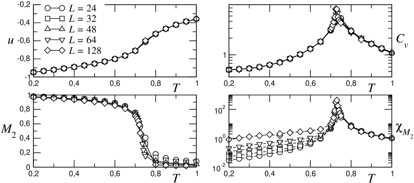
Figure 2: Energy, specific heat, order parameter $M_{2}$ and corresponding susceptibility $\chi_{M_{2}}$ vs $T$ for the $P_{4}\ O(2)$ model. The full lines are only guides for the eyes. The values of $k_{B}$ and $J$ have been fixed to unity.

Simulations are performed using a standard Wolff algorithm adapted to the expression of the nearest neighbour interaction [25, 26]. The spins are located on the vertices of a simple square lattice of size $L^{2}$ with periodic boundary conditions in the two directions. Usually $10^{6}$ equilibrium steps were used (measured as the number of flipped Wolff clusters) and $10^{6}$ Monte Carlo steps for the evaluation of thermal averages (the autocorrelation time at $k_{B}T/J=0.2$, $L=16$ is of order of $30$ MCS, hence the numbers of MC steps corresponds roughly to $3.10^{4}$ independent measurements for the smallest size). A first qualitative description of the behaviour of the system is provided by the temperature dependence of thermodynamic quantities [27]. The specific heat has a maximum which does not seem to increase substantially with the system size. This might be the sign of an essential singularity around a temperature $k_{B}T_{c}/J\simeq 0.70$. From the order parameter variation, a smooth transition is suspected, since there is no evolution toward a sharp jump. The susceptibility displays a non conventional behaviour at low temperature, increasing with the system size, which indicates a possible topological transition with a critical low temperature phase where the susceptibility diverges at any temperature.

3.2 Characterization of the low-temperature phase

We assume the existence of a critical phase at low temperatures as suggested by the temperature dependence results. The properties of the phase transition may be studied using

i) Standard Finite-Size Scaling technique (FSS): in the critical low temperature phase of a model which displays a topological transition, the physical quantities behave like at criticality for a second-order phase transition, with power law behaviours of the system size. The difference is that in the critical phase, the critical exponents depend on the temperature and for any temperature below the transition one has e.g.

$$M_{2}(T)\sim L^{-\frac{1}{2}\eta_{M_{2}}(T)}$$ (16)

$$\chi_{M_{2}}(T)\sim L^{2-\eta_{M_{2}}(T)}.$$ (17)

Here $\eta_{M_{2}}(T)$ denotes the correlation function critical exponent,

$$\langle Q_{2}(\cos(\theta_{{\bf r}_{1}}-\theta_{{\bf r}_{2}}))\rangle\sim|{\bf r}_{1}-{\bf r}_{2}|^{-\eta_{M_{2}}(T)}.$$ (18)

ii) Rescaling of the density profiles (or “Finite Shape Scaling”, FShS): conformally covariant density profiles or correlation functions are exepected at any temperature below the transition $T_{c}$. They transform according to $G(w_{1},w_{2})=|w^{\prime}(z_{1})|^{-x_{\sigma}}|w^{\prime}(z_{2})|^{-x_{\sigma}}G(z_{1},z_{2})$ through conformal mapping $w(z)$ where $w$ labels the lattice sites in the transformed geometry (the one where the computations are really performed), while $z$ refers to the infinite plane where the two-point correlations take the standard power-law expression $G(z_{1},z_{2})\sim|z_{1}-z_{2}|^{-\eta_{\sigma}}$), and $x_{\sigma}=\frac{1}{2}\eta_{\sigma}$ is the scaling dimension associated to the scaling field under consideration. Rather than two-point correlation functions, it is even more convenient to work with density profiles $m(w)$ in a finite system with symmetry breaking fields along some surfaces in order to induce a non-vanishing local order parameter in the bulk [28, 29, 30]. The density $m(w)$ will be $M_{2}({\bf r})=\langle Q_{2}({\bf S}_{\bf r}\cdot{\bf h}_{\partial\Lambda})\rangle$. In the case of a square lattice $\Lambda$ of size $L\times L$, with fixed boundary conditions along the four edges $\partial\Lambda$, one expects (details may be found e.g. in [29])

$$m(w) \sim [\kappa(w)]^{-\frac{1}{2}\eta_{\sigma}}$$

$$\kappa(w) = \Im{\rm m}\left[{\rm sn}\frac{2{\rm K}w}{L}\right]\times\left|\left(1-{\rm sn}^{2}\frac{2{\rm K}w}{L}\right)\left(1-k^{2}{\rm sn}^{2}\frac{2{\rm K}w}{L}\right)\right|^{-\frac{1}{2}}.$$ (19)

Another conformal mapping which has been applied to many two-dimensional critical systems is the logarithmic transformation $w(z)=\frac{L}{2\pi}\ln z=\frac{L}{2\pi}\ln\rho+i\frac{L\varphi}{2\pi}$ which maps the infinite plane onto an infinitely long cylinder of perimeter $L$. The correlation functions along the axis of the cylinder (let say in terms of the variable $u=\frac{L}{2\pi}\ln\rho$) decay exponentially at criticality, $G(u_{1},u_{2})\sim\exp[-(u_{2}-u_{1})/\xi]$, the correlation length amplitude on the strip being universal, $\xi=\frac{L}{\pi\eta}$ [31]. Simulations at different temperatures in a system of size $10\times 10000$ were performed and the correlation function exponent thus follows from the linear behaviour

$$\ln\langle Q_{2}[\cos(\theta_{u_{2}}-\theta_{u_{1}}]\rangle={\rm const}-\frac{\pi\eta_{M_{2}}}{L}(u_{2}-u_{1}).$$ (20)

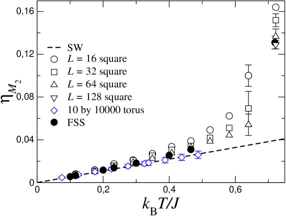
Figure 3: Temperature variation of the correlation function exponent $\eta_{M_{2}}(T)$ deduced from conformal rescaling (open symbols) and FSS (filled symbols). Open triangles and diamonds, which correspond the largest systems seem quite reliable. The dashed line shows the result of the spin-wave approximation $\eta_{M_{2}}(T)=\frac{11}{64}\frac{k_{B}T}{\pi J}$.

The resulting $\eta-$exponent deduced from these different techniques is shown in Fig. 3. The variation of $\eta$ with the temperature is very similar to the one observed in the case of the $XY$ model and confirms the QLRO nature of the LT phase of the model. The low temperature linear variation of this exponent is easily understood within the spin wave approximation. For $O(2)$ model with nearest neighbour interactions described by arbitrary polynomial in ${\bf S}_{\bf r}\cdot{\bf S}_{{\bf r}^{\prime}}$, one is led to an effective harmonic Hamiltonian $\frac{1}{2}J\sum_{({\bf r},{\bf r}^{\prime})}l(\theta_{\bf r}-\theta_{{\bf r}^{\prime}})^{2}$. It yields power-law correlations,

$$\langle\cos m(\theta_{{\bf r}_{1}}-\theta_{{\bf r}_{2}})\rangle={\rm e}^{-{\textstyle\frac{m^{2}}{2}}\langle(\theta_{{\bf r}_{1}}-\theta_{{\bf r}_{2}})^{2}\rangle}\sim|{\bf r}_{1}-{\bf r}_{2}|^{-\eta_{ml}}$$ (21)

with a decay exponent given by

$$\eta_{ml}=\frac{m^{2}}{l}\eta_{XY}=\frac{m^{2}}{2\pi Kl}.$$ (22)

The comparison is made visible in the figure (with $m=2$ and $l=128/11$), and as expected, the lower the temperature the better the SW approximation.

3.3 Critical behaviour at the deconfining transition

Not only the low temperature behaviour of $\eta$ is interesting, the precise value of the $\eta$ exponent at the BKT transition where some deconfining mechanism should lead to the proliferation of unbinded topological defects is also of interest, since it really describes the universality class of the transition. An accurate value of the transition temperature is first needed. We performed a study of the crossing point of $U_{4}$ Binder cumulant for very large statistics ($30\times 10^{6}$ MCS) and large system sizes (squares of $L=64$, 80, 96 and 128 with periodic boundary conditions). The results shown in Fig. 4 indicate a transition temperature of $k_{B}T_{\rm BKT}/J=0.7226$.

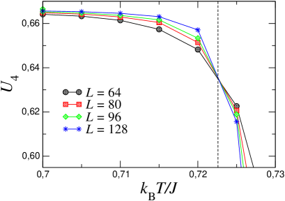
Figure 4: Left: Crossing of the Binder parameter at the deconfining transition at a temperature $k_{B}T_{\rm BKT}/J=0.7226$. Right: Size dependence of the correlation function exponent at $T_{\rm BKT}$ ($L=16$, 32, 64, 128) and extrapolation to the thermodynamic limit.

Then this temperature is used to perform Finite-Shape Scaling using the algebraic decay of density profiles inside a square with fixed bounday conditions. These simulations are time-consuming, since the autocorrelation time increases in the low temperature phase when $T$ evolves towards the deconfining transition and a rather large number of Monte Carlo steps is needed to get a satisfying number of independent measurements. For sizes $L=16$, 32, 64, we used $10^{6}$ MCS for thermalization and $30\cdot 10^{6}$ for measurements, while “only” $20\cdot 10^{6}$ for the largest size 128. The exponential decay of two-point correlation functions along the torus cannot be applied at the BKT transition, since the system size being quite larger than in a square geometry, the number of MC iterations required is by far too large. In Fig. 4 we plot the “effective” exponent $\eta_{\rm eff}(L)$ measured at $T_{\rm BKT}$ for different system sizes as a function of the inverse size. An estimate of the thermodynamic limit value ($L\to\infty$) can be made using a polynomial fit (the results of quadratic and cubic fits are respectively $0.118$ and $0.122$), but it is safer to keep the three largest sizes available, $L=32$, 64, and 128, for which a linear dependence of $\eta_{\rm eff}(L)$ with $L^{-1}$ is observed. Taking into account the error bars, crossing the extreme straight lines leads to the following value for the correlation function exponent at the deconfining transition

$$\eta_{M_{2}}(T_{\rm BKT})=0.122\pm 0.007.$$ (23)

This value is essentially half the Kosterlitz value for the $XY$ model.

4 Summary and open questions

The results obtained are essentially the following:

- The $P_{4}\ O(2)$ model displays a BKT-like transition with QLRO in the LT phase where SWA nicely fits the nematisation temperature-dependent exponents $\eta(T)$ when $T\to 0$.

- The value of the exponent at the deconfining transition is supposed to reach a universal value. The numerical estimate is close to $0.125$.

We believe that our conclusions are safe in which concerns the existence of a QLRO phase at low temperature. The results may be understood through a naive comparison with clock model in 2d. Increasing the order of the interaction polynomial indeed increases the number of deep wells which stabilise the relative orientation of neighbouring spins, and one is thus led to a system which is quite similar to a planar clock model with a finite number of states, unless the fact that here we keep a continuous spin symmetry which prevents from any “magnetic” long-range order at finite temperature. The clock model is in the Potts universality class when $q=3$, but at $q\geq 4$, it displays a QLRO phase before conventional ordering at lower temperatures [12]. Combining this analogy with the requirements of Mermin-Wagner-Hohenberg theorem for continuous spin symmetry gives a natural explanation for our results. For any type of nearest-neighbour interaction (in $P_{1}$, $P_{2}$ or $P_{4}$) the behaviour seems to be always described by a BKT-like transition. The similar observation that a two-component nematic model renormalises in two dimensions towards the $XY$ model was already reported in Ref. [32]. The transition is likely driven by a mechanism of condensation of defects, like in the $XY$ model, but due to the local $Z_{2}$ symmetry not only usual vortices carrying a charge $1$ are stable, but also disclination points carrying charges $1/2$ should be stable. The role of these defects might be studied in a similar way than in the recent work of Dutta and Roy [21], by the comparison of the the transition in the pure model and in a modified version where a chemical potential is artificially introduced in order to control the presence of defects.

Now, the observed value of the exponent $\eta$ at the transition temperature seems a bit strange. A naive application of the mechanism discussed in section 2 leads to a value two times larger. Apart from minor modifications, the same procedure applies. The Hamiltonian (15) is of the form (7) with $K$ replaced by $Kl$ which does not affect the universal properties, but changes the critical temperature by the same factor. The other modification comes from the local $Z_{2}$ symmetry in the nematic model. This changes the charges $n$ from integers to half-integers, which modifies the factor of $2\pi$ in equation (11) to $\pi/2$. The divergence of the perturbative term in (12) then occurs at $\frac{1}{2}\pi K_{c}l=4$, where the spin wave exponent (22) becomes $\eta_{c}=m^{2}/16$ which takes the value $\frac{1}{4}$ when $m=2$. We thus have a huge discrepancy of $100~{}\%$ between the numerical determination and this prediction! A probable source of this discrepancy may be in the mechanism involved. There are no negative charge in the nematic model, so the pair interaction has a different structure and a more refined analysis is therefore desirable.

Note added in proofs

We would like to thank S. Korshunov who draw our attention on a possible scenario explaining the discrepancy between the numerical value of $\eta$ and the prediction which follows from Kosterlitz-like arguments. Twenty years ago, he studied a similar planar $XY$ model with mixed interactions [33]. In the parameters space of the problem, there is a zone where, starting from the high temperature phase, a BKT transition is first observed and then at lower temperature occurs a phase transition governed by the presence of solitons. This latter transition belongs to the two-dimensional Ising model (IM) universality class. According to this scenario, ours results would thus correspond to this IM transition, but the quantity that we study does not correspond to the order parameter of this transition (hence the value of $\eta$ is not the usual $1/4$ of the IM universality class). QLRO would persist at higher temperatures, up to a limiting value where $\eta_{M_{2}}$ would indeed take its Kosterlitz-like value $m^{2}/16$.

References

- 1. N.D. Mermin and H. Wagner, Phys. Rev. Lett. 22, 1133 (1966).
- 2. P.C. Hohenberg, Phys. Rev. 158, 383 (1967).
- 3. V.L. Berezinskiĭ , Sov. Phys. JETP 32, 493 (1971).
- 4. J.M. Kosterlitz and D.J. Thouless, J. Phys. C: Solid State Phys. 6, 1181 (1973).
- 5. J.M. Kosterlitz, J. Phys. C: Solid State Phys. 7, 1046 (1974).
- 6. T.M. Rice, Phys. Rev. 140, A 1889 (1965).
- 7. D.R. Nelson, Defects and geometry in condensed matter physics, Cambridge University Press, Cambridge 2002.
- 8. A.M. Polyakov, Phys. Lett. 59B, 79 (1975).
- 9. E. Brézin and J. Zinn-Justin, Phys. Rev. B 14, 3110 (1976).
- 10. D.J. Amit, Field theory, the renormalization group and critical phenomena, World Scientific, Singapore 1984.
- 11. Yu.A. Izyumov and Yu.N. Skryabin, Statistical mechanics of magnetically ordered systems, Kluwer Academic Publishers, New-York 1988.
- 12. J.V. José, L.P. Kadanoff, S. Kirkpatrick and D.R. Nelson, Phys. Rev. B 16, 1217 (1977).
- 13. E. Domany, M. Schick and R.H. Swendsen, Phys. Rev. Lett. 52, 1535 (1984).
- 14. A. Jonsson, P. Minnhagen and M. Nylén, Phys. Rev. Lett. 70, 1327 (1993).
- 15. P.A. Lebwohl and G. Lasher, Phys. Rev. A 6, 426 (1973).
- 16. H. Kunz and G. Zumbach, Phys. Rev. B 46, 662 (1992).
- 17. H.W.J. Blöte, W. Guo and H.J. Hilhorst, Phys. Rev. Lett. 88, 047203 (2002).
- 18. S. Caracciolo and A. Pelissetto, Phys. Rev. E 66, 016120 (2002).
- 19. A.I. Fariñas-Sánchez, R. Paredes and B. Berche, Phys. Lett. A 308, 461 (2003).
- 20. R. Paredes, A.I. Fariñas-Sánchez and B. Berche, cond-mat/0401457.
- 21. S. Dutta and S.K. Roy, Phys. Rev. E 70, 066125 (2004).
- 22. A.C.D. van Enter and S.B. Shlosman, Phys. Rev. Lett. 28, 285702 (2002).
- 23. A.C.D. van Enter and S.B. Shlosman, Comm.Math. Phys. 255, 21 (2005).
- 24. K. Mukhopadhyay, A. Pal and S.K. Roy, Phys. Lett. A 253, 105 (1999).
- 25. A. Pal and S.K. Roy, Phys. Rev. E 67, 011705 (2003).
- 26. U. Wolff, Phys. Rev. Lett. 62, 362 (1989).
- 27. A.I. Farias Sanchez, R. Paredes V. and B. Berche, Phys. Rev. E 72, 031711 (2005).
- 28. B. Berche, A.I. Farias Sanchez and R. Paredes V., Europhys. Lett. 60, 539 (2002).
- 29. B. Berche, J Phys. A 36, 585 (2003).
- 30. B. Berche and L.N. Shchur, Pis’ma v ZhETF 79, 267 (2004), JETP Lett. 79, 213 (2004).
- 31. J.L. Cardy, J. Phys. A 17, L385 (1984).
- 32. D.R. Nelson and R.A. Pelcovits, Phys. Rev. B 16, 2191 (1977).
- 33. S.E. Koshunov, J. Phys. C: Solid State Phys. 19, 4427 (1986).