Kovacs effect in solvable model glasses

Abstract

The Kovacs protocol, based on the temperature shift experiment originally conceived by A.J. Kovacs and applied on glassy polymers [1], is implemented in an exactly solvable model with facilitated dynamics. This model is based on interacting fast and slow modes represented respectively by spherical spins and harmonic oscillator variables. Due to this fundamental property and to slow dynamics, the model reproduces the characteristic non-monotonic evolution known as the “Kovacs effect”, observed in polymers, spin glasses, in granular materials and models of molecular liquids, when similar experimental protocols are implemented.

1 Introduction

Glassy systems, being in an out-equilibrium condition, have properties which depend on their history. This is the ’memory’ of glasses. This property can manifest itself in striking ways, when specially devised experiments are made. One example is given by negative temperature cycles in spin glasses where the ac susceptibility, depending on both frequency and the age of the system, recovers the exact value it had before the negative temperature jump. A memory effect which shows up in a one-time observable, when a specific experimental protocol is implemented, is the so called “Kovacs effect” [1]. This effect has been the subject of a variety of recent investigations [2, 3, 4, 5, 6, 7]. The characteristic non-monotonic evolution of the observable under examination (the volume in the original Kovacs’ experiment), with the other thermodynamic variables held constant, shows clearly that a non-equilibrium state of the system cannot be fully characterized only by the (time-dependent) values of thermodynamic variables, but that further inner variables are needed to give a full description of the non-equilibrium state of the system. The memory in this case consists in these internal variables keeping track of the history of the system.
The purpose of this paper is to use a specific model for fragile glass to implement the protocol and get some insight into the Kovacs effect. We show that in spite of its simplicity, this model captures the phenomenology of the Kovacs effect and allows in specific regimes to obtain analytical expressions for the evolution of the variable of interest. This paper is organized as follows: in Section II we review the experimental protocol generating the effect, in Sections III and IV we introduce our model and use it to implement the protocol,in section V we draw out of this model some analytical results with final conclusions. An appendix collects all terms and coefficients employed in the main text.

2 Kovacs protocol

The experimental protocol, as originally designed by A. J. Kovacs in the ’60s [1], consists of three main steps:

1^st step

The system is equilibrated at a given high temperature $T_{i}$.

2^nd step

At time $t=0$ the system is quenched to a lower temperature $T_{l}$, close to or below the glass transition temperature, and it is let to evolve a period $t_{a}$. One then follows the evolution of the the proper thermodynamic variable (in the original Kovacs experiment this was the volume $V(t)$ of a sample of polyvinyl acetate, in our model it will be the “magnetization” $M_{1}(t)$).

3^rd step

After the time $t_{a}$, the volume, or other corresponding observable, has reached a value equal, by definition of $t_{a}$, to the equilibrium value corresponding to an intermediate temperature $T_{f}$ ($T_{l}<T_{f}<T_{i}$), i.e. such that $V_{T_{l}}(t_{a})\equiv V^{eq}_{T_{f}}$. At this time, the bath temperature is switched to $T_{f}$.

The pressure (or corresponding variable) is kept constant throughout the whole experiment.

Naively one would expect the observable under consideration, after the third step, to remain constant since it already has (at time $t=t_{a}^{+})$ its equilibrium value. But the system has not equilibrated yet and so the observable goes through a non monotonic evolution before relaxing back to its equilibrium value, showing a characteristic hump whose maximum increases with the magnitude of the final jump of temperature $T_{f}-T_{l}$ and occurs at a time which decreases with increasing $T_{f}-T_{l}$.

We want to implement this protocol on a model for both strong and fragile glass first introduced in [8]: the Harmonic Oscillators-Spherical Spins model (HOSS). This model is based on interacting fast and slow modes, this property turns out to be necessary for the memory effect, object of this paper, to occur.

3 The Harmonic Oscillator-Spherical Spin Model

The HOSS model contains a set of $N$ spins $S_{i}$ locally coupled to a set of $N$ harmonic oscillator $x_{i}$ according to the following hamiltonian:

$${\cal{H}}=\sum_{i=1}^{N}(\frac{K}{2}x_{i}^{2}-Hx_{i}-Jx_{i}S_{i}-LS_{i})$$ (1)

The spins have no fixed length but satisfy the spherical constraint: $\sum_{i=1}^{N}S_{i}^{2}=N$. The spin variables are assumed to relax on a much shorter time scale than the harmonic oscillator variables, so the oscillator variables are the slow modes and on their dynamical evolution the fast spin modes act just as noise. One can then integrate out the spin variables to obtain the following effective Hamiltonian for the oscillators (for details see [8], explicit expressions of undefined terms appearing in all equations hereafter are reported in the Appendix):

$$\frac{{\cal{H}}_{\it eff}(\{x_{i}\})}{N}=\frac{K}{2}M_{2}-HM_{1}-w_{T}(M_{1},M_{2})+\frac{T}{2}\log\left(\frac{w_{T}(M_{1},M_{2})+\frac{T}{2}}{\frac{T}{2}}\right)$$ (2)

which depends on the temperature and on the first and second moment of the oscillator variables, namely:

$$M_{1}=\frac{1}{N}\sum_{i=1}^{N}x_{i}\;\;\;,\;\;\;M_{2}=\frac{1}{N}\sum_{i=1}^{N}x_{i}^{2}$$ (3)

These variables encode the dynamics of the system which is implemented through a Monte Carlo parallel update of the oscillator variables:

$$x_{i}\to x_{i}+r_{i}/\sqrt{N}$$ (4)

The variables $r_{i}$ are normally distributed with zero mean value and variance $\sigma^{2}$. The update is accepted according to the Metropolis acceptance rule applied to the variation $\delta\epsilon$ of the energy of the oscillator variables, which is determined by ${\cal{H}}_{\it eff}$ and, in the limit of large $N$, is given by:

$$\frac{\delta\epsilon}{N}=\frac{K_{T}(M_{1},M_{2})}{2}\delta M_{2}-H_{T}(M_{1},M_{2})\delta M_{1}.$$ (5)

This simple model turns out to have a slow dynamics and can be solved analytically.

Following [8] one can derive the dynamical equations for $M_{1}$ and $M_{2}$

$$\dot{M}_{1} = \left[\frac{H_{T}(M_{1},M_{2})}{K_{T}(M_{1},M_{2})}-M_{1}\right]f_{T}(M_{1},M_{2})$$ (6)

$$\dot{M}_{2} = \frac{2}{K_{T}(M_{1},M_{2})}\left[I_{T}(M_{1},M_{2})+H_{T}(M_{1},M_{2})\dot{M}_{1}\right]$$

The stationary solutions of these equations coincide with the saddle point of the partition function of the whole system at equilibrium at temperature $T$ and are given by:

$$\bar{M}_{1} = \frac{H_{T}(\bar{M}_{1},\bar{M}_{2})}{K_{T}(\bar{M}_{1},\bar{M}_{2})}=\frac{\bar{H}_{T}}{\bar{K}_{T}}$$ (7)

$$\bar{M}_{2}-\bar{M}_{1}^{2} = \frac{T}{K_{T}(\bar{M}_{1},\bar{M}_{2})}=\frac{T}{\bar{K}_{T}}$$

with barred variables from now on indicating their equilibrium values.

3.1 Strong and Fragile Glasses with the HOSS model

In spite of its simplicity, the HOSS model allows to describe both strong and fragile glasses, characterized respectively by an Arrhenius or a Vogel-Fulcher law in the relaxation time. The following constraint on the configurations space is applied:

$$\mu_{2}=M_{2}-M_{1}^{2}-M_{0}\geq 0$$ (8)

When $M_{0}=0$ there exists a single global minimum in the configurations space of the oscillators, therefore the role of the constraint with $M_{0}>0$ is to avoid the existence of a “crystalline state” and to introduce a finite transition temperature. The stationary solutions for the dynamics with this constraint are given by:

$$\bar{M}_{1} = \frac{H_{T}(\bar{M}_{1},\bar{M}_{2})}{K_{T}(\bar{M}_{1},\bar{M}_{2})}=\frac{\bar{H}_{T}}{\bar{K}_{T}}$$ (9)

$$\bar{M}_{2}-\bar{M}_{1}^{2} = \left\{\rule{0.0pt}{21.33955pt}\begin{array}[]{c}\frac{T}{K_{T}(\bar{M}_{1},\bar{M}_{2})}=\frac{T}{\bar{K}_{T}}\;\;\;\;T>T_{k}\\ \\ M_{0}\;\;\;\;\;\;\;\;\;\;\;\;\;\;\;\;\;\;\;\;\;\;\;\;\;T\leq T_{k}\end{array}\right.$$ (13)

The temperature $T_{k}$ is determined by the further condition:

$$T_{k}=M_{0}\;K_{T_{k}}(\bar{M}_{1}^{T_{k}},\bar{M}_{2}^{T_{k}})=M_{0}\;\bar{K}_{T_{k}}.$$ (14)

This is the highest temperature at which the constraint is fulfilled, for smaller temperatures the system relaxes to equilibrium configurations which fulfill the constraint. For $T>T_{k}$ therefore the dynamics is not affected by the constraint. For $T\leq T_{k}$ the system eventually reaches a configuration which fulfills the constraint, when this happens it gets trapped for ever in such a configuration. This is equivalent to having a “Kauzmann-like” transition, occurring at $T=T_{k}$ with vanishing configuration entropy, meaning the system gets stuck forever in one single configuration fulfilling the constraint (see also: [9]).

When there is no constraint, i.e. when $M_{0}=0$, then $T_{k}=0$, if the Monte Carlo updates are done with Gaussian variables with constant variance $\sigma^{2}$, this model is characterized by an Arrhenius relaxation law:

$$\tau_{eq}\sim e^{\frac{A_{s}}{T}}$$ (15)

in so resembling the relaxation properties of strong glasses.

The HOSS model with constraint strictly positive ($M_{0}>0$) can easily be extended to describe fragile glasses by further introducing in the variance of the Monte Carlo update, the following dependence on the dynamics:

$$\sigma^{2}=8(M_{2}-M_{1}^{2})(M_{2}-M_{1}^{2}-M_{0})^{-\gamma}$$ (16)

In this case the relaxation time turns out to follow the generalized Vogel-Fulcher law:

$$\tau_{eq}\sim e^{A_{k}^{\gamma}/(T-T_{k})^{\gamma}}$$ (17)

The parameter $\gamma$ is introduced to make the best Vogel-Fulcher type fit for the relaxation time in experiments, making this model valid for a wide range of fragile glasses. When the temperature approaches the value $T_{k}$ defined by (14), from above, the system relaxes towards configurations close to the ones fulfilling the constraint. The variance $\sigma^{2}$ then tends to diverge, the updates become large and so unfavorable, meaning that almost every update of the oscillator variables is refused. This produces the diverging relaxation time following the Vogel-Fulcher law of Eq. (17).

4 Kovacs effect in the HOSS model

We implement the Kovacs protocol in the model above introduced for a fragile glass. The system is prepared at a temperature $T_{i}$ and quenched to a region of temperature close to the $T_{k}$, i.e. $T_{l}\gtrsim T_{k}$. Solving numerically Eqs. (6) we determine the evolution of the system in both step 2 and 3 of the protocol. In step 2 the time $t_{a}$, at which $M_{1}^{T_{l}}(t_{a})=\bar{M}_{1}^{T_{f}}$, is calculated so that:

$${M}_{1}^{T_{f}}(t_{a}^{+}) = \bar{M}_{1}^{T_{f}}$$ (18)

$${M}_{2}^{T_{f}}(t_{a}^{+}) = {M}_{2}^{T_{l}}(t_{a})$$

The evolution of the fractional ”magnetization”:

$$\vspace{-0.1cm}\Delta M_{1}(t)=\frac{M_{1}(t)-\bar{M}_{1}^{T_{f}}}{\bar{M}_{1}^{T_{f}}}\vspace{-0.1 cm}$$ (19)

after step 3 ($t>t_{a}$) for different values of $T_{l}$ is reported in Figs. 2 and 2 respectively for $\gamma=1$ and $\gamma=2$. The magnetic field $H$ is kept constant at the value $H=0.1$. In all the implementations of the protocol we use the values $J$=$K$=$1$, $L$=$0.1$ and $M_{0}$=$5$ for the other parameters of the model. This choice for the parameters and the value $H$=$0.1$ for the magnetic field fix (through Eqs. (9) and (14)) the Kauzmann temperature at the value $T_{k}$=$4.00248$.

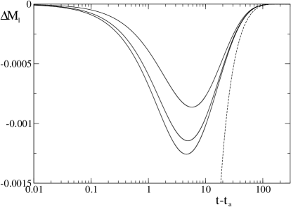
Figure 1: Fragile glass with $\gamma$=$1$ The Kovacs protocol is implemented with a quench of the system from temperature $T_{i}$=$10$ to $T_{l}$, and final switch (at $t$=$t_{a}^{+}$) to the intermediate temperature $T_{f}$=$4.3$. The continuous lines, starting from the lowest, refer to $T_{l}$=$4.005,4.05,4.15$, the dashed line refers to condition $T_{l}=T_{f}$, ( simple aging with no final temperature shift).

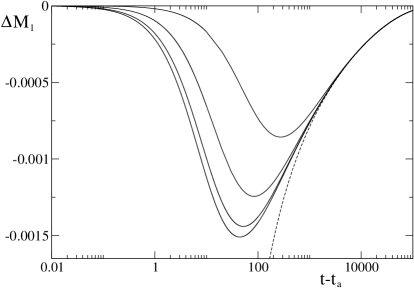
Figure 2: Fragile glass with $\gamma$=$2$. The Kovacs protocol is implemented with a quench of the system from temperature $T_{i}$=$10$ to $T_{l}$, and final switch (at $t$=$t_{a}^{+}$) to the intermediate temperature $T_{f}$=$4.3$. The continuous lines, starting from the lowest, refer to $T_{l}$=$4.005,4.05,4.15,4.25$, the dashed line refers to condition $T_{l}$=$T_{f}$ (simple aging with no final temperature shift).

Since the equilibrium value of $M_{1}$ decreases with increasing temperature (as opposed to what happens for instance with the volume) we observe a reversed ’Kovacs hump’. The curves keep the same properties typical of the Kovacs effect, the minima occur at a time which decreases and have a depth that increases with increasing magnitude of the final switch of temperature. As expected, since increasing $\gamma$ corresponds to further slowing the dynamics, the effect shows on a longer time scale in the case $\gamma=2$ as compared to $\gamma=1$.

Actually, since in the last step of the protocol: $M_{1}(t=t_{a})=\bar{M}_{1}^{T_{f}}$ and $f_{T_{f}}(M_{1},M_{2})$ is always positive, from the first of Eqs. (6) one soon realizes that the hump for this model can be either positive or negative, depending on the sign of the term:

$$\frac{H_{T_{f}}(\bar{M}_{1}^{T_{f}},M_{2})}{K_{T_{f}}(\bar{M}_{1}^{T_{f}},M_{2})}-\bar{M}_{1}^{T_{f}}$$ (20)

at $t=t_{a}^{+}$. This term is zero when $M_{1}=\bar{M}_{1}^{T_{f}},M_{2}=\bar{M}_{2}^{T_{f}}$, so one would expect $M_{2}(t=t_{a}^{+})=\bar{M}_{2}^{T_{f}}$ to be the border value determining the positivity or negativity of the hump. Since $H_{T_{f}}(\bar{M}_{1}^{T_{f}},M_{2})$ decreases with increasing $M_{2}$ while $K_{T_{f}}(\bar{M}_{1}^{T_{f}},M_{2})$ increases, it follows that the condition for a positive hump is:

$$M_{2}(t=t_{a}^{+})<\bar{M}_{2}^{T_{f}}$$ (21)

For shifts of temperature in a wide range close to the transition temperature $T_{k}$, where the dynamics is slower and the effect is expected to show up significantly on a long time scale, the condition $M_{2}(t=t_{a})>\bar{M}_{2}^{T_{f}}$ is always fulfilled and therefore a negative hump is expected.

5 Analytical solution in the long-time regime

In the previous Section we have shown, through a numerical solution of the dynamics, that the HOSS model reproduces the phenomenology of the Kovacs effect, showing the same qualitative properties of the Kovacs hump as obtained in experiments (see for ex. [1, 12]), in some other models with facilitated or kinetically constrained dynamics [7, 3] and in other different models [2, 4, 5, 6]. In this section we show that, by carefully choosing the working conditions in which the protocol is implemented, our model provides with an analytical solution for the evolution of the variable of interest.

5.1 Auxiliary variables

In order to ease calculations, as done in [9, 8] it is convenient to introduce the following variables:

$$\mu_{1}=\frac{H_{T}(M_{1},M_{2})}{K_{T}(M_{1},M_{2})}-M_{1}$$ (22)

$$\mu_{2}=M_{2}-M_{1}^{2}-M_{0}$$

for which the dynamical equations read:

$$\dot{\mu}_{1} = -JQ_{T}(M_{1},M_{2})I_{T}(M_{1},M_{2})-(1+DQ_{T}(M_{1},M_{2}))\mu_{1}f_{T}(M_{1},M_{2})$$ (23)

$$\dot{\mu}_{2} = \frac{2I_{T}(M_{1},M_{2})}{K_{T}(M_{1},M_{2})}+2\mu_{1}^{2}f_{T}(M_{1},M_{2})$$

We will choose to implement steps 2 and 3 of the protocol in a range of temperature very close to the Kauzmann temperature $T_{k}$. As exhaustively shown in [8, 11] in the long time regime the variable $\mu_{2}(t)$ decays logarithmically to its equilibrium value which is small for $T\sim T_{k}$. So, if $t_{a}$ is very large, the value of the variable $\mu_{2}(t)$, which is continuous at the jump, will be small enough to fulfill the condition for which the following equation is shown to be valid [8]:

$$\frac{d\mu_{1}}{d(\delta\mu_{2})}=(1+Q_{T}(M_{1},M_{2})D)\frac{(\bar{\mu}_{2}+\delta\mu_{2})^{-\gamma}}{\delta\mu_{2}}\mu_{1}-\frac{JQ_{T}(M_{1},M_{2})T}{2(M_{0}+\bar{\mu}_{2})}$$ (24)

where now the variable $\delta\mu_{2}(t)=\mu_{2}(t)-\bar{\mu}_{2}$ is used and barred variables always refer to equilibrium condition. Of course choosing $T_{l}$ close to $T_{k}$ and waiting a long time $t_{a}$ so that the system approaches equilibrium, allows only small temperature shifts for the final step of the protocol, meaning that also $T_{f}$ will be close to $T_{k}$. All the coefficients which appear in equation (24) (see Appendix for complete expressions) in the regime chosen, can be assumed constant and equal to their equilibrium values with a very good approximation. The equation can then be easily integrated to give:

$$\mu_{1}(\delta\mu_{2})=\exp\left[-\frac{\,{}_{2}F_{1}(\gamma,\gamma,\gamma+1,-\frac{\bar{\mu}_{2}}{\delta\mu_{2}})}{\gamma(\delta\mu_{2})^{\gamma}/A_{Q}}\right]\left(\mu_{1}^{+}B_{Q}^{\gamma}-C_{Q}\int_{\delta\mu_{2}^{+}}^{\delta\mu_{2}}dz\exp\left[\frac{\,{}_{2}F_{1}(\gamma,\gamma,\gamma+1,-\frac{\bar{\mu}_{2}}{z})}{\gamma z^{\gamma}/A_{Q}}\right]\right)$$

where the superscript ⁺ indicates $t=t_{a}^{+}$ and ${}_{2}F_{1}$ the hypergeometric function. This expression simplifies in cases $\gamma=1,\;3/2,\;2$. All these solutions and relative coefficients are reported in the appendix, here we limit ourselves to the case $\gamma=1$ which corresponds to ordinary Vogel-Fulcher relaxation law. In this case the solution is:

$$\mu_{1}(t)=\left(\frac{\delta\mu_{2}(t)}{\delta\mu_{2}(t)+\bar{\mu}_{2}}\right)^{\frac{A_{Q}}{\bar{\mu}_{2}}}\left[\mu_{1}^{+}\left(\frac{\delta\mu_{2}^{+}+\bar{\mu}_{2}}{\delta\mu_{2}^{+}}\right)^{\frac{A_{Q}}{\bar{\mu}_{2}}}-C_{Q}\int_{\delta\mu_{2}^{+}}^{\delta\mu_{2}(t)}dz\left(\frac{z}{z+\bar{\mu}_{2}}\right)^{-\frac{A_{Q}}{\bar{\mu}_{2}}}\right]$$ (25)

where:

$$\int_{a}^{b}dz\left(\frac{z}{z+\eta}\right)^{\alpha}=\frac{x^{\alpha+1}\;_{2}F_{1}(1-\alpha,-\alpha,2-\alpha,-\frac{x}{\eta})}{\eta^{\alpha}(1+\alpha)}|_{x=a}^{x=b}$$

One can then expand the variable of interest $M_{1}(t)$ in terms of $\mu_{1}$ and $\delta\mu_{2}$ and obtain the following expression for the Kovacs curves:

$$\delta M_{1}(t)=A_{T_{f}}^{1}(\bar{M}_{1}^{T_{f}},\bar{M}_{2}^{T_{f}})(\mu_{1}(t)-\mu_{1}^{+})+A_{T_{f}}^{2}(\bar{M}_{1}^{T_{f}},\bar{M}_{2}^{T_{f}})(\delta\mu_{2}(t)-\delta\mu_{2}^{+})$$ (26)

where the coefficients are approximately constant in the regime chosen and can be evaluated at equilibrium.

5.2 Short and intermediate $t-t_{a}$

For small $t-t_{a}$, a linear approximation for the variable $\delta\mu_{2}$, with slope given by the second equation of the set (23) evaluated at $t=t_{a}^{+}$, turns out to be very good. Inserting this expression in Eq. (25) to get $\mu_{1}(t)$ and then in Eq.(26) a good approximation of the first part of the hump for small and intermediate $t-t_{a}$ is obtained, as shown in Fig. 3.

5.3 Intermediate and long $t-t_{a}$

When $t-t_{a}$ is very large, we can use Eq. (25) and the pre-asymptotic approximation for $\mu_{2}(t)$ (see: [8])

$$\mu_{2}(t)=\left(\log(t/t_{0})+\frac{1}{2}\log(\log(t/t_{0}))\right)^{-1/\gamma}$$ (27)

Inserting this expression in Eq. (25) to get $\mu_{1}(t)$ and then in Eq.(26), a good approximation for the hump and the tail of the Kovacs curves is obtained. In Fig. 3 we show the agreement between the analytical expression so obtained and the numerical solution.

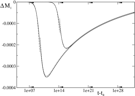
Figure 3: Comparison between numerical solution (continuous lines) for the Kovacs’ curves and the approximate analytical solution at short-intermediate (dot-dashed line) and intermediate-long time (dashed line). The protocol is implemented between $T_{i}=10$ and $T_{f}=4.018$. The curves starting from the lowest refer to $T_{l}=4.005$, $4.008$. ($H=0.1$, $T_{k}=4.00248$)

6 Conclusion

We have shown that a simple mode with constrained dynamics like the HOSS model, is rich enough to reproduce the Kovacs memory effect, even allowing to obtain analytical expression for the Kovacs hump in a long time regime. The Kovacs effect is observed in many experiments and models, showing common qualitative properties which we have found to be shared also by the model analyzed in this paper. The quantitative properties depend on the particular system or model analyzed.

As far as it concerns the HOSS model, it turns out that for the slow modes, i.e. the oscillator variables, fixing the overall average value, the magnetization $M_{1}$, does not prevent the existence of memory encoded in the variable $M_{2}$, which keeps track of the history of the system. The equilibrium value of $M_{2}$ increases with temperature while the equilibrium value of $M_{1}$ decreases with increasing temperature. Therefore after the final switch of temperature, since $M_{2}(t_{a})>\bar{M}_{2}^{T_{f}}$, the variable $M_{2}$ has a value corresponding to an equilibrium condition at a higher temperature (memory of the initial state at temperature $T_{i}$) so driving the system towards a condition corresponding to a higher temperature, i.e. smaller values of $M_{1}$, determining the hump.

It is important to stress that a fundamental ingredient in the HOSS model, besides the slow dynamics which originates from the Monte Carlo parallel update, is the interaction between slow and fast modes. Due to this interaction the equilibrium configurations of the oscillator variables at a given temperature are determined by both $M_{2}$ and $M_{1}$, the first and second moment of their distribution, whose dynamical evolution is interdependent. When such interaction is turned off (by setting $J=0$ ) essentially only one variable is sufficient to describe the equilibrium configurations and the dynamics of the system, and the memory effect is lost. In this respect this model constitutes an improvement to the so-called oscillator model [13] within which such memory effect cannot be reproduced. In the present model one can also study temperature cycle experiments of the type carried out in spin glasses (see. [14]), leaving room for further research.
More details on this subject can be found in Ref. [15].

G.A. and L.L. gratefully acknowledge the European network DYGLAGEMEM for financial support.

Appendix A

In this Appendix we report all the explicit expressions for terms appearing in the text. In Eqs. (2), (5) and (6) we have:

$$w_{T}(M_{1},M_{2})=\sqrt{J^{2}M_{2}+2JLM_{1}+L^{2}+T^{2}/4}$$

$$K_{T}(M_{1},M_{2})=K-\frac{J^{2}}{w_{T}(M_{1},M_{2})+T/2}$$

$$H_{T}(M_{1},M_{2})=H+\frac{JL}{w_{T}(M_{1},M_{2})+T/2}$$

$$f_{T}(M_{1},M_{2})=\frac{\sigma^{2}K_{T}(M_{1},M_{2})}{2T}Erfc\left[\tilde{\alpha}_{T}(M_{1},M_{2})\right]\cdot\exp\left[\tilde{\alpha}_{T}^{2}(M_{1},M_{2})-\alpha_{T}^{2}(M_{1},M_{2})\right]$$

$$I_{T}(M_{1},M_{2})=\frac{\sigma^{2}K_{T}(M_{1},M_{2})}{4}Erfc\left[\alpha_{T}(M_{1},M_{2})\right]+\left(\frac{T}{2}-K_{T}(M_{1},M_{2})\tilde{w}_{T}(M_{1},M_{2})\right)f_{T}(M_{1},M_{2})$$

where:

$$\tilde{w}_{T}(M_{1},M_{2})=M_{2}-M_{1}^{2}+(\frac{H_{T}(M_{1},M_{2})}{K_{T}(M_{1},M_{2})}-M_{1})^{2}$$

$$\alpha_{T}(M_{1},M_{2})=\sqrt{\frac{\sigma^{2}}{8\tilde{w}_{T}(M_{1},M_{2})}}$$

$$\frac{\tilde{\alpha}_{T}(M_{1},M_{2})}{\alpha_{T}(M_{1},M_{2})}=\frac{2K_{T}(M_{1},M_{2})\tilde{w}_{T}(M_{1},M_{2})}{T}-1$$

In Eqs. (15), (17), (24), (5.1), (25) and (26):

$$A_{s} = \frac{\sigma^{2}\bar{K}_{T}}{8}$$

$$D = JH+LK=JH_{T}+LK_{T}$$

$$Q_{T}(M_{1},M_{2}) = \frac{J^{2}D}{K_{T}^{3}w_{T}(w_{T}+T/2)^{2}}$$

$$P_{T}(M_{1},M_{2}) = \frac{J^{4}(M_{2}-M_{1}^{2})}{2K_{T}w_{T}(w_{T}+T/2)^{2}}$$

$$A_{k} = \frac{\bar{K}_{T_{k}}(K-\bar{K}_{T_{k}})(1+D\bar{Q}_{T_{k}}+\bar{P}_{T_{k}})}{(K-\bar{K}_{T_{k}})(1+D\bar{Q}_{T_{k}})-\bar{K}_{T_{k}}\bar{Q}_{T_{k}}}$$

$${}_{2}F_{1}(a,b,c,z) = \frac{\Gamma(c)}{\Gamma(a)\Gamma(b)}\sum_{n=0}^{\infty}\frac{\Gamma(a+n)\Gamma(b+n)}{\Gamma(c+n)}\frac{z^{n}}{n!}$$

$$A_{Q} = 1+Q_{T_{f}}(\bar{M}_{1}^{T_{f}},\bar{M}_{2}^{T_{f}})D=1+\bar{Q}_{T_{f}}D$$

$$B_{Q}^{\gamma} = \exp[A_{Q}\frac{\,{}_{2}F_{1}(\gamma,\gamma,\gamma+1,-\frac{\bar{\mu}_{2}}{\delta\mu_{2}^{+}})}{\gamma(\delta\mu_{2}^{+})^{\gamma}}]$$

$$C_{Q} = \frac{JQ_{T_{f}}(\bar{M}_{1}^{T_{f}},\bar{M}_{2}^{T_{f}})T_{f}}{2(M_{0}+\bar{\mu}_{2})}=\frac{J\bar{Q}_{T_{f}}T_{f}}{2(M_{0}+\bar{\mu}_{2})}$$

$$A^{1}_{T}(M_{1},M_{2}) = \frac{(w_{T}+T/2)K_{T}}{M_{1}(JM_{1}+L+(w_{T}+T/2)K_{T})}$$

$$A^{2}_{T}(M_{1},M_{2}) = 2M_{1}A^{1}_{T}(M_{1},M_{2})$$

$$t_{0} = \frac{\sqrt{\pi}}{8\gamma}\frac{1+D\bar{Q}_{T}}{1+D\bar{Q}_{T}+\bar{P}_{T}}$$

References

- [1] A. J. Kovacs, Adv. Polym. Sci. 3, 394 (1963); A. J. Kovacs, J.J. Aklonis, J.M. Hutchinson, A.R. Ramos, J. Pol. Sci. 17, 1097 (1979)
- [2] L. Berthier, J-P. Bouchaud, Phys. Rev. B 66, 054404 (2002)
- [3] A. Buhot, J. Phys. A: Math. Gen. 36, 12367 (2003)
- [4] E M Bertin, J-P Bouchaud, J-M Drouffe and C Godr che, J. Phys. A: Math. Gen. 36, 10701, (2003)
- [5] L. F. Cugliandolo, G. Lozano, H. Lozza, Eur. Phys. J. B 41, 87 (2004)
- [6] S. Mossa and F. Sciortino, Phys. Rev. Lett. 92, 045504 (2004)
- [7] J. J. Arenzon and M. Sellitto, Eur. Phys. J. B 42, 543-548, 2004
- [8] L. Leuzzi, Th. M. Nieuwenhuizen, Phys. Rev. E 64, 011508 (2001)
- [9] Th. M. Nieuwenhuizen, cond-mat/9911052
- [10] Th. M. Nieuwenhuizen, Phys. Rev. E 61, 267 (2000)
- [11] Luca Leuzzi, Thermodynamics of glassy systems, PhD Thesis, Universiteit van Amsterdam, (2002).
- [12] C. Josserand, A. Tkachenko, D. M. Mueth, H. M. Jaeger, Phys. Rev. Lett. 85, 3632 (2000)
- [13] LL Bonilla, FG Padilla and F. Ritort, Physica A 250, 315 (1998)
- [14] E. Vincent, J. Hamman, M. Ocio, J-P. Bouchaud and L.F. Cugliandolo, in Complex Behaviour of Glassy Systems, Springer Verlag Lecture Notes in Physics Vol. 492, M. Rubi editor, 1997, pp.184-219
- [15] G. Aquino, L. Leuzzi and Th. M. Nieuwenhuizen, “Kovacs effect in a fragile glass model”, cond-mat/0511654, submitted to Phys. Rev. B