Frozen local hole approximation

Abstract

The frozen local hole approximation (FLHA) is an adiabatic approximation which is aimed to simplify the correlation calculations of valence and conduction bands of solids and polymers or, more generally, of the ionization potentials and electron affinities of any large systems. Within this approximation correlated local hole states (CLHSs) are explicitely generated by correlating local Hartree-Fock (HF) hole states, i. e. ($N$-1)-particle determinants in which the electron has been removed from a local occupied orbital. The hole orbital and its occupancy is kept frozen during these correlation calculations, implying a rather stringent configuration selection. Effective Hamilton matrix elements are then evaluated with the above CLHSs; diagonalization finally yields the desired correlation corrections for the cationic hole states. We compare and analyze the results of the FLHA with the results of a full MRCI(SD) (multi-reference configuration interaction with single and double excitations) calculation for two prototype model systems, (H₂)_n ladders and H–(Be)_n–H chains. Excellent numerical agreement between the two approaches is found. Comparing the FLHA with a full correlation treatment in the framework of quasi-degenerate variational perturbation theory reveals that the leading contributions in the two approaches are identical. In the same way it could be shown that replacing a correlation calculation around a frozen local hole is in fact equivalent, up to first order, to perform a much less demanding SCF (self-consistent field) calculation around the hole to relax all other occupied orbitals. Thus, both, the FLHA and the above SCF approximation, are well-justified and provide a very promising and efficient alternative to fully correlated wavefunction-based treatments of the valence and conduction bands in extended systems.

I Introduction

In the last decade, increasing interest in wavefunction-based correlation methods for excited states in extended systems can be observed Gräfenstein et al. (1993, 1997); de Graaf et al. (1999); Albrecht et al. (2000); Albrecht and Igarashi (2001); Albrecht (2002); Hozoi et al. (2002, 2003); V.Bezugly and Birkenheuer (2004); Buth et al. (2005). This is because one can rely on the very sophisticated numerical methods for molecules which are well-established in quantum chemistry. These methods are conceptually very clear and allow for systematic improvement: based on self-consistent field calculations, electron correlation can be included successively by considering determinants of increasing excitation order in configuration interaction (CI) or related procedures. They yield approximate correlated wavefunctions from which all quantities of interest can be derived.

Of course, wavefunction-based methods are computationally very demanding. In order to arrive at manageable schemes for the description of solids or other extended systems, local orbitals have to be introduced and the local character of electron correlation must rigorously be exploited. Among these local approaches Pisani (2002) one can distinguish local MP2 (Møller-Plesset perturbation theory up to 2^nd order) and coupled electron pair or coupled cluster schemes Saebø and Pulay (1987); Fink and Staemmler (1995); Hampel and Werner (1996); Schütz et al. (1999); Sun and Bartlett (1996); Ayala et al. (2001); Pisani et al. (2005), methods which are based on a Green’s function formalism Albrecht (2002); Buth et al. (2005) and techniques which use local Hamiltonian matrix elements Gräfenstein et al. (1993, 1997); Albrecht et al. (2000); V.Bezugly and Birkenheuer (2004) or other partitioning concepts Stoll (1992a, b, c); Paulus et al. (1995); Fulde (2002); Willnauer and Birkenheuer (2004); Angeli et al. (2003); Kitaura et al. (1999); Fedorov and Kitaura (2004); Mochizuki et al. (2005); Borini et al. (2005). Whereas the first-mentioned methods work in infinite systems and aim to truncate the excitation space by an appropriate configuration selection scheme, the effective Hamiltonian approach as well as the other partitioning schemes assemble the correlation effects from finite subsystems (embedded fragments) which are finally transfered to the infinite system. Most of these methods focus on ground state properties, only the Green’s function and local Hamiltonian approaches are explicitely designed for excited states. In particular, the local Hamiltonian approach has been used in the past quite successfully to describe the correlation effects on the band structure of covalent solids Gräfenstein et al. (1993, 1997); Albrecht et al. (2000) and polymers V.Bezugly and Birkenheuer (2004). Yet, this approach is quite involved and a more simpler, approximative way of computing the local Hamiltonian has been proposed recently by our lab Birkenheuer et al. (2005).

In this work we want to analyze the guiding approximations introduced in that recent approach, and therefore address the question to which extent it is possible to simplify the correlation calculations by focusing on “frozen” local hole configurations although, in reality, the electron hole is usually delocalized over the entire system. Intuitively, this frozen local hole approximation, is guided by the idea that the shape of the correlation hole which is carried along by a traveling electron is essentially invariant and is thus following the electron hole adiabatically.

A related approach is the frozen core hole approximation Rössler and Staemmler (2003) for the calculation of core-hole states where the core hole orbital is frozen and all other orbitals are allowed to relax during an Hartree-Fock calculation. Such a local view on core holes in bulk materials is also adopted in other wavefunction-based investigations on excited core hole states de Graaf et al. (1997); de Vries et al. (2002). While it seems quite natural to describe core holes in that way, although in solids even core orbitals are Bloch waves, it is much less obvious that a frozen local hole treatment should also be possible for delocalized valence hole states.

In the following, we will outline the theoretical background of the frozen local hole approximation (for valence holes) and then present and analyze the numerical results obtained for two model systems, namely (H₂)_n ladders and H–(Be)_n–H chains. These two examples have been chosen to represent the two cases of prevailing van der Waals and predominantly covalent binding. Finally, an analytical, perturbative analysis of the frozen local hole approximation is given.

II Theoretical background

Starting point for our correlation calculations is the Hartree-Fock (HF) ground state Slater determinant $|\Phi_{0}^{N}\rangle$ and energy $E_{0}^{N}$ of the $N$-particle system. The canonical HF orbitals $|\nu\rangle$ with orbital energies $\epsilon_{\nu}$ are divided into the $N/2$ energetically lowest-lying orbitals which are occupied in $|\Phi_{0}^{N}\rangle$ and the unoccupied, virtual orbitals. Furthermore, the occupied orbitals are subdivided into core and valence orbitals depending on whether they are kept frozen or are active during the subsequent correlation calculation. Within these orbital groups we will switch between delocalized canonical orbitals and localized orbitals, $\{|\nu\rangle\}$ and $\{|a\rangle\}$, using unitary transformations, such as

$$|a\rangle=\sum_{\nu}|\nu\rangle U_{\nu a}$$ (1)

for the occupied orbitals. In order to find the correlated cationic ($N$-1)-particle states of the system in mind, one first constructs the so-called reference states $|\Phi_{i}^{N-1}\rangle$ of the system by removing one electron out of one of the valence orbitals $|i\rangle$: $|\Phi_{i}^{N-1}\rangle=\hat{c}_{i}|\Phi_{0}^{N}\rangle$. The so generated canonical hole states $|\Phi_{\nu}^{N-1}\rangle$ and local hole states $|\Phi_{a}^{N-1}\rangle$ are connected via

$$|\Phi_{\nu}^{N-1}\rangle=\sum_{a}|\Phi_{a}^{N-1}\rangle(U^{-1})_{a\nu}^{\ast}=\sum_{a}|\Phi_{a}^{N-1}\rangle U_{\nu a}\quad$$ (2)

Since we are only dealing with cationic states here we will omit the upper index ($N$-1) in the following. The canonical hole states are the eigenstates of the CI matrix in the reference space. They describe the hole states of the system according to Koopmans’ theorem Koopmans (1933).

Including correlation effects one arrives at correlated wave functions $|\Psi_{\nu}\rangle$ with energies $E_{\nu}$. In analogy to Eq. (2) we then define so-called correlated local hole states $|\Psi_{a}\rangle$ (see Fig. 1)

$$|\Psi_{a}\rangle:=\sum_{\nu}|\Psi_{\nu}\rangle U_{\nu a}^{\ast}$$ (3)

and an effective Hamilton matrix $\underline{\underline{H}}^{\rm eff}=(H_{ab}^{\rm eff})$ with

$$H_{ab}^{\rm eff}:=\langle\Psi_{a}|\hat{H}|\Psi_{b}\rangle=\sum_{\nu}U_{\nu a}E_{\nu}U_{\nu b}^{\ast}\quad.$$ (4)

The effective Hamiltonian $\hat{H}^{\rm eff}$ is constructed such that diagonalizing its local matrix representation $\underline{\underline{H}}^{\rm eff}$ precisely yields the desired correlated energies $E_{\nu}$ of the cationic states. Thus, provided one knows the correlated local hole states $|\Psi_{a}\rangle$ defined in Eq. (3), one can find the cationic energies by simply solving a small eigenvalue problem.

Figure 1: Relation between the delocalized hole state on the Hartree-Fock level $|\Phi_{\nu}\rangle$ and the corresponding correlated states $|\Psi_{\nu}\rangle$, and their localized counterparts, $|\Phi_{a}\rangle$ and $|\Psi_{a}\rangle$, respectively. Within the frozen local hole approximation (FLHA) approximate correlated local hole states $|\tilde{\Psi}_{a}\rangle$ are constructed without explicit reference to the true correlated states $|\Psi_{\nu}\rangle$.

Within our frozen local hole approach we do not follow the three-step process depicted in Fig. 1 but directly generate approximate correlated local hole states (CLHSs) $|\tilde{\Psi}_{a}\rangle$ by performing separate correlation calculations for each reference state $|\Phi_{a}\rangle$ during which the hole in the localized orbital $|a\rangle$ is kept frozen. This implies a configuration selection where only those configurations are used in which the hole in $|a\rangle$ is maintained. In the case of an CI(SD) (CI with single and double excitations) calculation the approximate localized hole states $|\tilde{\Psi}_{a}\rangle$ take on the following form:

$$|\tilde{\Psi}_{a}\rangle=\alpha_{a}|\Phi_{a}\rangle+\sum_{x,v}\alpha_{a,x}^{v}|\Phi_{a,x}^{v}\rangle+\sum_{\begin{subarray}{c}x,x^{\prime}\\ v,v^{\prime}\end{subarray}}\alpha_{a,x,x^{\prime}}^{v,v^{\prime}}|\Phi_{a,x,x^{\prime}}^{v,v^{\prime}}\rangle\;.$$ (5)

The indices $x,x^{\prime}\in\{\bar{a},b,\bar{b},...\}$ run over all the remaining valence electrons, with $\bar{a}$ being the electron with opposite spin to the removed electron $a$. $v,v^{\prime}$ denote the electrons in the virtual orbitals. Thus, e. g., $|\Phi_{a,\bar{a}}^{v}\rangle$ is the 2h1p configuration with no electrons remaining in the spatial orbital associated with $a$ whereas $|\Phi_{a,b}^{v}\rangle$ contains holes in two different spatial orbitals. Obviously, the configuration spaces for the different hole states $|\tilde{\Psi}_{a}\rangle$ are overlapping. Excited configurations with holes in two or more valence orbitals $|a\rangle$, $|b\rangle$, … are, in fact, present in the correlation calculations of each reference state $|\Phi_{a}\rangle$, $|\Phi_{b}\rangle$, $\ldots$ (see Fig. 6). As we will see in detail later, this fact does not harm the procedure. On the contrary, it is important to build up the correlation effects in the final, delocalized hole states properly through a suitable mixing of the configurations in the final diagonalization step of the effective Hamiltonian (4),

$$|\tilde{\Psi}_{\nu}\rangle=\sum_{a}\lambda_{a}(\nu)|\tilde{\Psi}_{a}\rangle\quad\quad\mbox{where}$$ (6)

$$\sum_{b}H_{ab}^{\rm eff}\lambda_{b}(\nu)=\tilde{E}_{\nu}\sum_{b}S_{ab}\lambda_{b}(\nu)\quad.$$ (7)

Note, that the individual approximated CLHSs $|\tilde{\Psi}_{a}\rangle$ are not orthonormal with respect to each other. Thus, one has to solve a generalized eigenvalue problem here (with $S_{ab}=\langle\tilde{\Psi}_{a}|\tilde{\Psi}_{b}\rangle$ being the overlap matrix) in order to arrive at the approximate canonical hole states $|\tilde{\Psi}_{\nu}\rangle$ and the approximate hole state energies $\tilde{E}_{\nu}$.

III Applications

As first applications of the frozen local hole approximation (FLHA) we choose two simple model systems, (H₂)_n ladders (see Fig. 2) and linear H–(Be)_n–H chains, for which we compare and analyze the results of the approximation with the results of the corresponding complete multi-reference CI(SD) (MRCI(SD)) calculation. All results are obtained by using the MOLPRO program package Werner et al. (2003), in particular the MRCI(SD) option Werner and Knowles (1988); Knowles and Werner (1988, 1992). For the calculations sp cc-pVDZ basis sets by Dunning T. H. Dunning (1989) are used for H and Be except for the terminating H atoms in the Be chains which are described by a reduced s cc-pVDZ basis. The Be–H distance has been set to $1.37$ Å which is the equilibrium distance found in all neutral chains of length $n$=4–10. The computation of the Hartree-Fock ground state of the neutral system $|\Phi^{N}_{0}\rangle$ yields the canonical Hartree-Fock orbitals. The set of valence orbitals is subsequently localized by means of the Foster-Boys procedure Foster and Boys (1960) and is used for the construction of the localized hole states $\{|\Phi_{a}\rangle\}$. Each $|\Phi_{a}\rangle$ is then separately correlated in a CI(SD) calculation with the above-described configuration selection, where only those single and double excitations are allowed with a hole in the localized orbital $|a\rangle$. In order to achieve this configuration restriction within the MOLPRO program, one has to declare all valence and unoccupied orbitals as active orbitals. The maximum number of active orbitals is fixed to 32 in the MOLPRO code, which only allowed us to handle relatively small chains and basis sets chosen here. Nevertheless, the effects of the approximation can be studied very well in these model systems.

Figure 2: Geometry of the (H₂)_n ladders used in this paper. The H₂ bond length is fixed at its molecular value of $R=0.7417$ Å; the distance between the H₂ units is varied during the calculations.

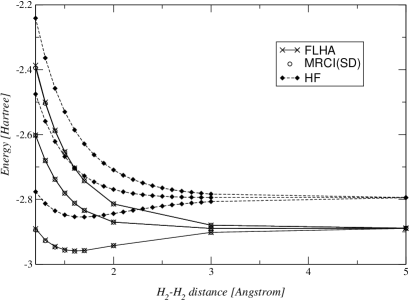
Figure 3: Total Hartree-Fock, MRCI(SD) and FLHA energies of (H₂)${}_{3}^{+}$ as a function of the H₂–H₂ distance.

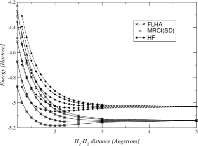
Figure 4: Total Hartree-Fock, MRCI(SD) and FLHA energies of (H₂)${}_{5}^{+}$ as a function of the H₂–H₂ distance.

The results for the (H₂)${}_{3}^{+}$ and (H₂)${}_{5}^{+}$ ladders are shown in Figs. 3 and 4. Here, the total energies of the hole states on the HF, the MRCI(SD) and the FLHA level are depicted in dependence of the distance between the H₂ units. In accordance with the number of valence orbitals, and thus possible hole states, we find three and five low-lying cationic states of (H₂)${}_{3}^{+}$ and (H₂)${}_{5}^{+}$, respectively. In their lowest states the cationic (H₂)_n ladders are stable. Compared to the HF data, very pronounced correlation effects are observed: In the case of the (H₂)${}_{3}^{+}$ chain the lowest-lying state is lowered by about 2.9 eV at its equilibrium distance, which is slightly shifted from $R_{\rm eq}=1.7$ to $1.6$ Å, and the potential well is deepened from 1.6 to 1.9 eV. Also for the high-lying states of (H₂)${}_{3}^{+}$ and the states of (H₂)${}_{5}^{+}$ states we find an overall energetical lowering of about 3 eV through correlation. The most important finding in the present context, however, is that all the described effects are very well accounted for by the frozen local hole approximation. The FLHA curves follow the MRCI reference data very closely with the only noticeable slight deviations at the outer left edge of the potential curves.

In order to make sure that this excellent agreement is not only an artefact of the relatively weak van der Waals binding between the H₂ units, we choose the predominantly covalently bound H–(Be)_n–H chains as second application. For all systems considered, H–(Be)₃–H through H–(Be)₅–H, the FLHA and the “exact” MRCI(SD) data agree very well. In the following, we only want to discuss in detail the results for the smallest system Be₃H${}_{2}^{+}$ shown in Fig. 5. The calculated correlated potential energy curves for the two lowest cationic states exhibit shallow minima at Be–Be distances of $R_{\rm eq}=2.3$ and $2.4$ Å. For the most stable cationic state of Be₃H₂ the correlation energies vary from about 1.1 eV at the minima to about 1.5 eV for small and large Be–Be distances.

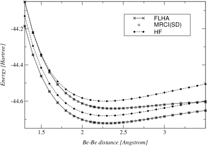
Figure 5: Total Hartree-Fock, MRCI(SD) and FLHA energies for Be₃H${}_{2}^{+}$ in dependence of the Be–Be distance.

The dominating configurations of the two lowest cationic states are the two reference configurations $|\Phi_{a}\rangle$ and $|\Phi_{b}\rangle$ which result from taking one electron out of one of the highest occupied molecular orbitals (HOMOs) of the HF determinant. The corresponding localized orbitals are centered at the Be–Be bonds (see top row of Fig. 7). Within the FLHA two configuration spaces I and II are constructed, built upon the two reference configurations $|\Phi_{a}\rangle$ and $|\Phi_{b}\rangle$. They are shown schematically in Fig. 6. Clearly, the two configuration spaces strongly overlap. For this simple example with two reference configurations only, all mixed (single-excited) 2h1p configurations $|\Phi_{a,b}^{v}\rangle$, $|\Phi_{\bar{a},b}^{v}\rangle$ and $|\Phi_{a,\bar{b}}^{v}\rangle$ and all (doubly-excited) 3h2p configurations $|\Phi_{a,x,x^{\prime}}^{v,v^{\prime}}\rangle$ and $|\Phi_{b,x,x^{\prime}}^{v,v^{\prime}}\rangle$ fall into the overlap region. Nevertheless, very important configurations, especially the reference configurations themselves, lie in only one of the spaces. That is why this very simple example is already suited to show the main features of the approximation. Strictly speaking, the single determinants $|\Phi_{a,\bar{b}}^{v}\rangle$ only belong to space I (as the $|\Phi_{\bar{a},b}^{v}\rangle$ only belong to space II). But since MOLPRO uses spin-adapted excitations these two types of single determinants always come in singlet and triplet-like linear combinations $(|\Phi_{a,\bar{b}}^{v}\rangle\pm|\Phi_{\bar{a},b}^{v}\rangle)/\sqrt{2}$ and are thus both attributed to the overlap region I $\cap$ II.

In the present example, no substantial saving in the computational cost can be gained from using the FLHA, since we substitute the single MRCI(SD) calculation by two CI calculations with configuration spaces of almost the same size as the original one. But this will change dramatically with bigger systems because a given configuration can be found in at most three different configuration spaces. E. g., the double excited configuration $|\Phi_{a,b,c}^{v,v^{\prime}}\rangle$ would only be part of the configuration spaces generated from the reference configurations $|\Phi_{a}\rangle$, $|\Phi_{b}\rangle$ and $|\Phi_{c}\rangle$. Once suitable cut-off criteria are introduced, the configuration spaces of each reference configuration remain finite no matter how large the systems becomes; and since the number of these spaces only grow linearly with system size the FLHA directly leads to an ${\cal O}(N)$ method.

Figure 6: Sketch of the overlapping configuration spaces I and II for a system with two valence orbitals and two hole states. The nomenclature is the same as in Eq. (5).

Coming back to the discussion of the Be₃H₂ results, only a few configurations with noticeable weights ($>0.05$) are found in the approximated correlated local hole states $|\tilde{\Psi}_{a}\rangle$ and $|\tilde{\Psi}_{b}\rangle$ (Eq. (5)). The same holds true for the “full” canonical MRCI wave functions, $|\Psi^{\rm MRCI}_{1}\rangle$ and $|\Psi^{\rm MRCI}_{2}\rangle$. In order to enable an analysis of the individual correlation contributions, we also localize the virtual orbitals, although this is by no means a prerequisite of our FLHA. All relevant configurations contain excitations into one of the four pair-wise degenerated virtual orbitals shown in Fig. 7. The first pair, named $c_{x}^{\ast}$ and $c_{y}^{\ast}$, is localized at the central Be atom, the other pair, $a^{\ast}$ and $b^{\ast}$, represents anti-bonding orbitals on the two Be–Be bonds.

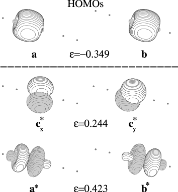
Figure 7: Localized highest occupied orbitals (HOMOs) of Be₃H${}_{2}^{+}$ together with those localized virtual orbitals which are involved in the most relevant configurations of the approximate correlated local hole states $|\tilde{\Psi}_{a}\rangle$ and $|\tilde{\Psi}_{b}\rangle$. The Hartree-Fock orbital energies $\epsilon$ of each energetically degenerate pair of orbitals are given as well.

In Table 1 we summarize the CI coefficients $\alpha_{I}$ and $\beta_{I}$ of the most relevant contributions to the approximate CLHSs $|\tilde{\Psi}_{a}\rangle$ and $|\tilde{\Psi}_{b}\rangle$, as well as the CI coefficients $(\alpha_{I}\pm\beta_{I})/\sqrt{2}$ of the approximated wave functions $\tilde{\Psi}_{\nu}$ of the hole states 1 and 2 as resulting from the diagonalization of the effective Hamiltonian, a ($2\times 2$) matrix, here. The latter CI coefficients are compared with those of the “exact” MRCI wave functions, $\alpha_{1,I}^{\rm MRCI}$ and $\alpha_{2,I}^{\rm MRCI}$. For all spin-adapted single determinants considered here: the reference configurations, the single and double excitations into the anti-bonding orbitals $a^{\ast}$ and $b^{\ast}$ and the 3h2p configurations involving the orbitals $c_{x}^{\ast}$ and $c_{y}^{\ast}$, an excellent agreement is found between the approximate and the “exact” CI coefficients of the holes states with deviations well below 10% in most of the cases. In contrast to our initial expectation, no cancellation of artificial, orbital-relaxation-based contributions in the FLHA wave functions occur. All configurations which are important in the CLHSs also contribute significantly to (at least) one of the final hole states $|\tilde{\Psi}_{1}\rangle$ and $|\tilde{\Psi}_{2}\rangle$. Apparently, the ultimate diagonalization step just mixes the individual contributions in such a way that the delocalized nature of the hole states is recovered, precisely as one would expect for an adiabatic approximation.

IV Perturbative analysis

To understand, why the frozen local hole approximation (FLHA) works so well, we switch from the MRCI level of theory to quasi-degenerate variational perturbation theory (QDVPT) Cave and Davidson (1988) and try to find the leading contributions in both, the “exact” hole state and the approximate hole states according to the FLHA. Within QDVPT the correlated wave functions $|\Psi_{\nu}\rangle$ of a system are written as

$$|\Psi_{\nu}\rangle=\hat{\Omega}|\Psi^{\cal M}_{\nu}\rangle$$ (8)

where $|\Psi^{\cal M}_{\nu}\rangle=\hat{P}|\Psi_{\nu}\rangle$ are the projections of the correlated wave functions $|\Psi_{\nu}\rangle$ onto the space ${\cal M}$ spanned by the local Hartree-Fock hole configurations $\{|\Phi_{a}\rangle\}$, and $\hat{\Omega}$ is an operator which acts on the “model space” ${\cal M}$ and provides the full, correlated wave functions $|\Psi_{\nu}\rangle$. It is assumed that the $|\Psi_{\nu}\rangle$ are those eigenstates of the hole system which are dominated by the single determinants forming the model space and, in particular, that the projections $|\Psi^{\cal M}_{\nu}\rangle$ remain linear independent. In fact,

$$\hat{\Omega}=\hat{P}+\hat{Q}\hat{\Omega}\quad\mbox{with}\quad\hat{Q}\,\hat{\Omega}=\sum_{I,a}|\Phi_{I}\rangle\Omega_{Ia}\langle\Phi_{a}|$$ (9)

where $\hat{Q}=\sum_{I}|\Phi_{I}\rangle\langle\Phi_{I}|$ is the projector onto the orthogonal complement of the model space and the configurations $|\Phi_{I}\rangle$ run over all single, double and higher excitations one can form from the local model space configurations $\{|\Phi_{a}\rangle\}$.

In first order perturbation theory the wave operator $\hat{\Omega}$ is given by Cave and Davidson (1988)

$$\hat{\Omega} = \sum_{c}|\Phi_{c}\rangle\langle\Phi_{c}|$$

$$+ \sum_{c}\sum_{a<b,v}|\Phi_{ab}^{v}\rangle\,\frac{\langle vc||ab\rangle}{\varepsilon_{v}-\varepsilon_{a}-\varepsilon_{b}+\varepsilon_{c}}\langle\,\Phi_{c}|\quad.$$

We take the zeroth-order Hamiltonian $H^{0}$ to consist of the diagonal terms of the Fock operator only, i. e., $H^{0}_{ij}=\delta_{ij}\varepsilon_{i}$ with $\varepsilon_{i}=F_{ii}$. The perturbation then contains both, the off-diagonal terms $F_{ij}=\langle\varphi_{i}|\hat{F}|\varphi_{j}\rangle\;,\;i\neq j$ of the Fock operator $\hat{F}$ and the usual two-electron contributions $\langle ij||kl\rangle-\sum^{\rm occ}_{a}\langle ia||ja\rangle$. Here and in the following, indices $a$, $b$, $\ldots$ are understood to run over occupied localized orbitals while indices $v$, $w$, $\ldots$ run over virtual orbitals. For arbitrary orbitals indices $i$, $j$, $\ldots$ are used. The 12,12 notation

$$\langle ij||kl\rangle=\langle ij|\hat{g}|kl\rangle-\langle ij|\hat{g}|lk\rangle\quad\quad\mbox{with}$$ (11)

$$\langle ij|\hat{g}|kl\rangle=\int\!\!\!\int\varphi^{\ast}_{i}(1)\varphi^{\ast}_{j}(2)\>r_{12}^{-1}\>\varphi_{k}(1)\varphi_{l}(2)\>d1\,d2$$

is employed throughout. The $|\varphi_{i}\rangle$ are the (localized) Hartree-Fock orbitals of the neutral $N$-electron system. Using that form of the wave operator as variational ansatz for the eigenstates of the hole system, i. e.

$$|\Psi_{\nu}\rangle=\hat{\Omega}\big{[}\>\sum_{a}\lambda_{a}(\nu)|\Phi_{a}\rangle\>\big{]}=\sum_{a}\lambda_{a}(\nu)\>\hat{\Omega}|\Phi_{a}\rangle\quad,$$ (12)

leads to the following effective secular matrix

$$H^{\rm eff}_{ef} := \langle\,\hat{\Omega}\!\big{[}\Phi_{e}\big{]}|\hat{H}|\,\hat{\Omega}\!\big{[}\Phi_{f}\big{]}\rangle$$ (13)

$$= -F_{fe}$$

$$+\sum_{a<b,v}W_{e|ab,f}^{\;\;v}\>\langle vf||ab\rangle$$

$$+\sum_{a<b,v}W_{e,ab|f}^{\;\;v}\>\langle ab||ve\rangle$$

$$+\sum_{a<b,v}\sum_{c<d,w}W_{e,ab|cd,f}^{\;\;v\;\;\,w}\>\langle ab||ve\rangle\>\langle wf||cd\rangle$$

with

$$W_{e|ab,f}^{\;\;v} = \frac{\langle\Phi_{e}|\hat{H}|\Phi_{ab}^{v}\rangle}{(\varepsilon_{v}-\varepsilon_{a}-\varepsilon_{b}+\varepsilon_{f})}$$ (15)

$$W_{e,ab|f}^{\;\;v} = \frac{\langle\Phi_{ab}^{v}|\hat{H}|\Phi_{f}\rangle}{(\varepsilon_{v}-\varepsilon_{a}-\varepsilon_{b}+\varepsilon_{e})}\;=\;(W_{f|ab,e}^{\;\;\,v})^{\ast}$$

$$W_{e,ab|cd,f}^{\;\;v\;\;\,w} = \frac{\langle\Phi_{ab}^{v}|\hat{H}|\Phi_{cd}^{w}\rangle}{(\varepsilon_{v}-\varepsilon_{a}-\varepsilon_{b}+\varepsilon_{e})\>(\varepsilon_{w}-\varepsilon_{c}-\varepsilon_{d}+\varepsilon_{f})}\;\;.$$

This is not what is usually done in QDVPT, but to preceed this way allows to find the direct link to the frozen local hole approximation we are looking for.

In the first step of the FLHA, the model space configurations and the excited configurations are restricted to those determinants which already contain a hole in a particular local occupied orbital $|\varphi_{h}\rangle$, such that the wave operator reduces to

$$\hat{\Omega}^{\rm FLH}(h)=|\Phi_{h}\rangle\langle\Phi_{h}|\>+\sum_{a\neq h,v}|\Phi_{ah}^{v}\rangle\,\frac{\langle vh||ah\rangle}{\varepsilon_{v}-\varepsilon_{a}}\langle\Phi_{h}|\quad.$$ (16)

Only single excitations $|\Phi_{ah}^{v}\rangle$ with respect to the given local hole configuration $|\Phi_{h}\rangle$ show up here. Inspection of Eq. (IV) reveals that these restricted wave operators are precisely the leading terms in the full wave operator $\hat{\Omega}$, in the sense that

$$\hat{\Omega}=\sum_{h}\hat{\Omega}^{\rm FLH}(h)+\hat{\Pi}$$ (17)

where the remainder

$$\hat{\Pi}=\sum_{a<b,v}\sum_{c\not\in\{a,b\}}|\Phi_{ab}^{v}\rangle\,\frac{\langle vc||ab\rangle}{\varepsilon_{v}-\varepsilon_{a}-\varepsilon_{b}+\varepsilon_{c}}\,\langle\Phi_{c}|$$ (18)

contains all terms in which the three occupied spin orbitals $|a\rangle$, $|b\rangle$, and $|c\rangle$ are all different, while the leading terms are made up by all those contributions in which two of the hole indices coincide.

The final secular matrix of the frozen local hole approach,

$$H^{\rm FLH}_{gh}:=\langle\,\hat{\Omega}^{\rm FLH}(g)\!\big{[}\Phi_{g}\big{]}|\hat{H}|\,\hat{\Omega}^{\rm FLH}(h)\!\big{[}\Phi_{h}\big{]}\rangle\quad,$$ (19)

is then given by

$$H^{\rm FLH}_{gh} = -F_{hg}$$

$$+\sum_{c\neq h,w}W_{g|ch,h}^{\;\;w}\langle wh||ch\rangle$$

$$+\sum_{a\neq g,v}W_{g,ag|h}^{\;\;v}\langle ag||vg\rangle$$

$$+\sum_{a\neq g,v}\sum_{c\neq h,w}W_{g,ag|ch,h}^{\;\;v\;\;\;w}\langle ag||vg\rangle\langle wh||ch\rangle$$

which is again precisely the leading coinciding-hole-indices part of the full effective Hamiltonian $H^{\rm eff}_{gh}$ (despite the always present zeroth-order contribution $-F_{hg}$). Thus, up to first order perturbation theory the FLHA can be understood as a simple neglection of all three-distinct-spin-orbital contributions to the wave operator $\hat{\Omega}$ and the resulting effective Hamiltonian.

A further simplification of the FLHA can be achieved by treating the ($N$-1)-particle system with a frozen local hole on the Hartree-Fock level only. This has already been done with some success in our “simplified method” to correlation effects in band structures Birkenheuer et al. (2005). Orbital relaxation around the localized hole is the only effect which can be accounted for in this approach and we want to analyze here, to which extent the correlation effects in the ($N$-1)-particle system can be mimicked this way.

Removal of an electron from a fixed localized occupied spin orbital $|\varphi_{h}\rangle$ leads to the following modified Fock operator $\hat{F}^{\rm FLH}(h)$,

$$\langle i|\hat{F}^{\rm FLH}(h)|j\rangle = F_{ij}-\langle ih||jh\rangle\>=\>\delta_{ij}\,\varepsilon_{i}+\langle i|V|j\rangle$$

$$\mbox{with}\quad\langle i|V|j\rangle = (1-\delta_{ij})\,F_{ij}-\langle ih||jh\rangle$$ (21)

Up to first order in the perturbation potential $V$ the relaxed Hartree-Fock orbitals $|\tilde{\varphi}_{i}(h)\rangle$ which result from diagonalizing $\hat{F}^{\rm FLH}(h)$ under the constraint that $|\tilde{\varphi}_{h}\rangle$ remains unchanged read

$$|\tilde{\varphi}_{i}(h)\rangle=\left\{\begin{array}[]{ll}\displaystyle{|\varphi_{i}\rangle-\sum_{j\not\in\{i,h\}}|\varphi_{j}\rangle\,\frac{\langle j|V|i\rangle}{\varepsilon_{j}-\varepsilon_{i}}}&\quad\mbox{for }i\neq h\\ |\varphi_{h}\rangle&\quad\mbox{else}\end{array}\right.$$ (22)

and the corresponding Slater determinant

$$|\Phi_{h}^{\rm SCF}\rangle := \frac{(-1)^{N-h}}{\sqrt{(N-1)!}}\times$$

$$\mbox{det}(\tilde{\varphi}_{1}(h),\ldots,\tilde{\varphi}_{h-1}(h),\tilde{\varphi}_{h+1}(h),\ldots,\tilde{\varphi}_{N}(h))$$

becomes

$$|\Phi_{h}^{\rm SCF}\rangle=|\Phi_{h}\rangle-\sum_{a\neq h}\sum_{j\not\in\{a,h\}}|\Phi_{ah}^{j}\rangle\,\frac{\langle j|V|a\rangle}{\varepsilon_{j}-\varepsilon_{a}}+{\cal O}(V^{2})\quad.$$ (24)

Excitations into occupied spin orbitals $|\varphi_{j}\rangle$ other than $|\varphi_{a}\rangle$ and $|\varphi_{h}\rangle$ are not possible in the 2h1p configurations $|\Phi_{ah}^{j}\rangle$. Thus, $j$ only runs over the virtual orbitals and one has

$$|\Phi_{h}^{\rm SCF}\rangle = |\Phi_{h}\rangle+\sum_{a\neq h,v}|\Phi_{ah}^{v}\rangle\,\frac{\langle vh||ah\rangle}{\varepsilon_{v}-\varepsilon_{a}}+{\cal O}(V^{2})$$ (25)

$$= \hat{\Omega}^{\rm FLH}(h)|\Phi_{h}\rangle+{\cal O}(V^{2})$$ (26)

Obviously, up to first order, the local frozen hole wave function obtained on the Hartree-Fock level is identical to the fully correlated local hole state $|\tilde{\Psi}_{h}\rangle=\hat{\Omega}^{\rm FLH}(h)|\Phi_{h}\rangle$ of the system (see Eq. (16)). This result is somewhat surprising, at first glance, because it tells, that what formally looks like pure orbital relaxation around a frozen local defect, is actually bare electron correlation. It also tells, that performing a Hartree-Fock calculation around a frozen local hole rather than a much more demanding wavefunction-based correlation calculations is a rather promising approximation.

V Conclusions

The so-called frozen local hole approximation (FLHA) has been analyzed in this study. It presents a method that allows to perform correlation calculations for cationic and anionic ($N$$\pm$1)-electron systems in a much more efficient way than running a full quantum chemical correlation calculation such as MRCI(SD). In this work we were focusing on cationic holes states, but, in a totally analogue way, the approximation can also be applied to anionic electron attachment states (as done in Ref. Birkenheuer et al. (2005)).

The FLHA is a two step procedure: In the first step, the electron to be removed is assumed to reside in a given, fixed local occupied orbital and standard wavefunction-based correlation calculations are performed in order to find the correlation hole around each of these local holes. Because of the frozen character of the given hole orbital the configuration space is substantially reduced in these correlation calculations. Therefore, the approximation is a perfect, linear scaling divide-and-conquer approach. In the second step, the many-body Hamiltonian matrix elements with the correlated local hole states generated in the first step are evaluated and the resulting effective Hamiltonian matrix is diagonalized. In this way, the hole can delocalize over the whole system to form proper Bloch states. Hence, the FLHA can be understood as an adiabatic treatment, in which the shape of the correlation hole around each electron hole is kept fixed during the final hybridization of the correlated local hole states.

It has been shown numerically, for two sample systems, $({\rm H}_{2})_{n}$ ladder chains and hydrogen terminated linear H–(Be)_n–H chains, that the FLHA performs astonishingly well. Potential energy curves have been calculated on the MRCI(SD) level of theory, and deviations of at most 0.1 eV between a full correlation calculations and the frozen local hole approach were found, both, for the van der Waals bound H₂ chains and for the covalent Be chains.

Using quasi-degenerate variational perturbation theory, it was possible to demonstrate that the FLHA indeed assembles all leading terms of a full correlation calculation. Actually, the approximation consists in a neglection of all three-distinct-hole-site contributions over those where (at least) two hole orbitals coincide. Furthermore, it could be shown that the correlation calculation around a frozen local hole can very well be replaced by a numerically much less demanding SCF calculation. In first order perturbation theory the resulting orbital relaxations are totally equivalent to the correlation effects around a frozen local hole.

Table 1: Analysis of the most relevant configurations in the two lowest correlated cationic hole states $|\Psi_{1}\rangle$ and $|\Psi_{2}\rangle$ of Be₃H₂. The first columns give the occupation numbers of the involved spatial orbitals (Fig. 7). The indices $S$ and $T$ refer to spin-adapted configurations with a singlet and triplet-like linear combination of the remaining electrons in a and b, respectively. The next two columns show the CI coefficients $\alpha_{I}$ and $\beta_{I}$ of the approximate correlated hole states $|\tilde{\Psi}_{a}\rangle$ and $|\tilde{\Psi}_{b}\rangle$, respectively, as defined in Eq. (5), followed by the CI coefficients of the hole states $|\tilde{\Psi}_{\nu=1}\rangle$ and $|\tilde{\Psi}_{\nu=2}\rangle$ after the diagonalization step (7). They are to be compared to the CI coefficients $\alpha_{1,I}^{{\rm MRCI}}$ and $\alpha_{2,I}^{{\rm MRCI}}$ of the “exact” MRCI wave functions $|\Psi^{\rm MRCI}_{\nu=1}\rangle$ and $|\Psi^{\rm MRCI}_{\nu=2}\rangle$.

configuration $I$						$|\tilde{\Psi}_{a}\rangle$	$|\tilde{\Psi}_{b}\rangle$	$|\tilde{\Psi}_{1}\rangle$	$|\Psi^{\rm MRCI}_{1}\rangle$	$|\tilde{\Psi}_{2}\rangle$	$|\Psi^{\rm MRCI}_{2}\rangle$	type of configuration
a	b	$|$	a∗	b∗	c∗	$\alpha_{I}$	$\beta_{I}$	$\frac{1}{\sqrt{2}}(\alpha_{I}+\beta_{I})$	$\alpha^{\rm MRCI}_{1,I}$	$\frac{1}{\sqrt{2}}(\alpha_{I}-\beta_{I})$	$\alpha^{\rm MRCI}_{2,I}$
1	2	$|$	0	0	0	-0.9528	–	-0.6737	-0.6767	-0.6737	-0.6682	ref. configuration $|\Phi_{a}\rangle$
2	1	$|$	0	0	0	–	-0.9528	-0.6737	-0.6767	-0.6737	-0.6682	ref. configuration $|\Phi_{b}\rangle$
1	1	$|$	1	0	0S	-0.0824	-0.0901	-0.0054	-0.0052	-0.1220	-0.1450
1	1	$|$	1	0	0T	-0.0595	-0.1028	-0.1148	-0.1026	-0.0306	-0.0307
1	1	$|$	0	1	0S	-0.0901	-0.0824	-0.0054	-0.0052	-0.1220	-0.1450	mixed 2h1p configurations
1	1	$|$	0	1	0T	-0.1028	-0.0595	-0.1148	-0.1026	-0.0306	-0.0307
0	2	$|$	0	1	0	-0.0507	–	-0.0359	-0.0302	-0.0359	-0.0451	type I 2h1p configurations
2	0	$|$	1	0	0	–	-0.0507	-0.0359	-0.0302	-0.0359	-0.0451	type II 2h1p configurations
1	0	$|$	0	0	2	-0.0651	-0.0298	-0.0671	-0.0617	-0.0250	-0.0297
0	1	$|$	0	0	2	-0.0298	-0.0651	-0.0671	-0.0617	-0.0250	-0.0297	3h2p configurations

References

- Gräfenstein et al. (1993) J. Gräfenstein, H. Stoll, and P. Fulde, Chem. Phys. Lett. 215, 611 (1993).
- Gräfenstein et al. (1997) J. Gräfenstein, H. Stoll, and P. Fulde, Phys. Rev. B 55, 13588 (1997).
- Albrecht et al. (2000) M. Albrecht, P. Fulde, and H. Stoll, Chem. Phys. Lett. 319, 355 (2000).
- Albrecht and Igarashi (2001) M. Albrecht and J.-I. Igarashi, J. Phys. Soc. Jap. 70, 1035 (2001).
- Albrecht (2002) M. Albrecht, Theo. Chem. Acc. 107, 71 (2002).
- V.Bezugly and Birkenheuer (2004) V.Bezugly and U. Birkenheuer, Chem. Phys. Lett. 399, 57 (2004).
- de Graaf et al. (1999) C. de Graaf, C. Sousa, and R. Broer, J. Mol. Struc. (TheoChem) 458, 53 (1999).
- Hozoi et al. (2002) L. Hozoi, A. H. de Vries, A. B. van Oosten, R. Broer, J. Cabrero, and C. de Graaf, Phys. Rev. Lett. 89, 076407 (2002).
- Hozoi et al. (2003) L. Hozoi, C. Presura, C. de Graaf, and R. Broer, Phys. Rev. B 67, 035117 (2003).
- Buth et al. (2005) C. Buth, U. Birkenheuer, M. Albrecht, and P. Fulde, Phys. Rev. B 72, 195107 (2005).
- Pisani (2002) C. Pisani, J. Mol. Struct. (TheoChem) 621, 141 (2002).
- Saebø and Pulay (1987) S. Saebø and P. Pulay, J. Chem. Phys. 86, 914 (1987).
- Hampel and Werner (1996) C. Hampel and H.-J. Werner, J. Chem. Phys. 104, 6286 (1996).
- Schütz et al. (1999) M. Schütz, G. Hetzer, and H.-J. Werner, J. Chem. Phys. 111, 5691 (1999).
- Sun and Bartlett (1996) J.-Q. Sun and R. J. Bartlett, J. Chem. Phys. 104, 8553 (1996).
- Ayala et al. (2001) P. Y. Ayala, K. N. Kudin, and G. E. Scuseria, J. Chem. Phys. 115, 9698 (2001).
- Pisani et al. (2005) C. Pisani, M. Busse, G. Capecchi, S. Casassa, R. Dovesi, L. Maschio, C. Zicovich-Wilson, and M. Schütz, J. Chem. Phys. 122, 094113 (2005).
- Fink and Staemmler (1995) K. Fink and V. Staemmler, J. Chem. Phys. 103, 2603 (1995).
- Kitaura et al. (1999) K. Kitaura, E. Ikeo, T. Asada, T. Nakano, and M. Uebayasi, Chem. Phys. Lett. 313, 701 (1999).
- Fedorov and Kitaura (2004) D. G. Fedorov and K. Kitaura, J. Chem. Phys. 121, 2483 (2004).
- Mochizuki et al. (2005) Y. Mochizuki, S. Koikegami, S. Amari, K. Segawa, K. Kitaura, and T. Nakano, Chem. Phys. Lett.) 406, 283 (2005).
- Stoll (1992a) H. Stoll, Chem. Phys. Lett. 191, 548 (1992a).
- Stoll (1992b) H. Stoll, Phys. Rev. B) B46, 6700 (1992b).
- Stoll (1992c) H. Stoll, J. Chem. Phys. 97, 8449 (1992c).
- Paulus et al. (1995) B. Paulus, P. Fulde, and H. Stoll, Phys. Rev. B 51, 10572 (1995).
- Fulde (2002) P. Fulde, Adv. Phys. 51, 909 (2002).
- Willnauer and Birkenheuer (2004) C. Willnauer and U. Birkenheuer, J. Chem. Phys. 120, 11910 (2004).
- Angeli et al. (2003) C. Angeli, C. J. Calzado, R. Cimiraglia, S. Evangelisti, N. Guihéry, T. Leininger, J.-P. Malrieu, D. Maynau, J. V. P. Ruiz, and M. Sparta, Mol. Phys. 101, 1389 (2003).
- Borini et al. (2005) S. Borini, D. Maynau, and S. Evangelisti, J. Comput. Chem. 26, 1042 (2005).
- Birkenheuer et al. (2005) U. Birkenheuer, P. Fulde, and H. Stoll, Theo. Chem. Acc. (2005), submitted, arXiv:cond-mat/0511626.
- Rössler and Staemmler (2003) N. Rössler and V. Staemmler, Phys. Chem. Chem. Phys. 5, 3580 (2003).
- de Graaf et al. (1997) C. de Graaf, R. Broer, W. C. Nieuwpoort, and P. S. Bagus, Chem. Phys. Lett. 272, 341 (1997).
- de Vries et al. (2002) A. H. de Vries, L. Hozoi, R. Broer, and P. S. Bagus, Phys. Rev. B 66, 035108 (2002).
- Koopmans (1933) T. Koopmans, Physica 1, 104 (1933).
- Werner et al. (2003) H.-J. Werner, P. J. Knowles, R. Lindh, M. Schütz, P. Celani, T. Korona, F. R. Manby, G. Rauhut, R. D. Amos, A. Bernhardsson, et al., Molpro, version 2002.6, a package of ab initio programs (2003), see http://www.molpro.net.
- Werner and Knowles (1988) H.-J. Werner and P. J. Knowles, J. Chem. Phys. 89, 5803 (1988).
- Knowles and Werner (1988) P. J. Knowles and H.-J. Werner, Chem. Phys. Letters 145, 514 (1988).
- Knowles and Werner (1992) P. J. Knowles and H.-J. Werner, Theor. Chim. Acta 84, 95 (1992).
- T. H. Dunning (1989) J. T. H. Dunning, J. Chem. Phys. 90, 1007 (1989).
- Foster and Boys (1960) J. M. Foster and S. F. Boys, Rev. Mod. Phys. 32, 300 (1960).
- Cave and Davidson (1988) R. J. Cave and E. R. Davidson, J. Chem. Phys. 89, 6798 (1988).