The dynamic exponent of the Ising model on negatively curved surfaces

Abstract

We investigate the dynamic critical exponent of the two-dimensional Ising model that is defined on a curved surface with constant negative curvature. By using the short-time relaxation method, we find the quantitative alteration of the dynamic exponent from the known value for the planar Ising model. This phenomenon is attributed to the fact that the Ising lattices embedded on negatively curved surfaces act as those in an infinite dimension, thus yielding the dynamic exponent deduced from the mean-field theory. We further demonstrate that the static critical exponent for the correlation length exhibits the mean-field exponent, which agrees with the existing results obtained by canonical Monte Carlo simulations.

1 Introduction

Physics on curved surfaces is an intriguing subject especially with regard to second-order phase transition. This is because the non-zero curvature of the underlying surface converts the essential symmetries of the embedded physical system through a spatial fluctuation of the metric. The two-dimensional (2$d$) Ising model defined on a curved surface is an exemplary system. While the interest in this model originates from its relevance to the quantum gravity theory [1, 2, 3, 4, 5], it is presently motivated by the remarkable advances in nanotechnology that enables the production of curved magnetic layers of desired shapes [6, 7]. Earlier studies have revealed that the Ising model defined on a curved surface exhibits peculiar critical behaviors that differ from those of the planar Ising model [8, 9, 10, 11, 12, 13]. In particular, on a surface with a constant negative curvature, several static critical exponents have been proven to deviate quantitatively from the exact solution for the planar model [14]. The latter results indicate the occurrence of a novel universality class of the $2d$ Ising model induced by surface curvature.

Successful findings on the static critical properties motivate the study of the dynamic critical behaviors of the Ising model on a curved surface. The dynamic scaling hypothesis states that, in the vicinity of the critical temperature $T_{c}$, the thermodynamic quantities $O$ of finite-sized systems obey the dynamic scaling form as follows [15, 16]:

$$O(t,\epsilon,L)=L^{\phi}\cdot{\cal O}\left(tL^{-z},\;\epsilon L^{1/\nu}\right),$$ (1)

where $t$ is the dynamic time variable, $\epsilon=|T-T_{c}|/T_{c}$ the reduced temperature, $L$ the linear dimension of the system, and ${\cal O}$ the universal scaling function. $\phi$ and $\nu$ are static critical exponents, while $z$ is the dynamic critical exponent that takes the value of $z\simeq 2.2$ in the planar Ising model (See Refs. [17, 18, 19] and references therein). The main concern is whether the finite surface curvature leads to a change in the value of $z$ given above. It should be noted that the curvature-induced alteration of static critical exponents observed in Ref. [14] has no bearing on this problem, since the value of $z$ that characterizes the dynamic universality class of the system is generally independent of its static universality class. Determination of $z$ is, therefore, crucial to obtain a better understanding of the curvature effect on the critical behavior of the $2d$ Ising model.

In the present study, we numerically investigate the dynamic critical exponent of the Ising model defined on a curved surface with constant negative curvature. The short-time relaxation (STR) method [18, 20, 21, 22] and the finite-size scaling analysis reveal that the dynamic exponent on the curved surface exhibits a value that is different from that for the planar Ising model. This quantitative change in the dynamic exponent results from the peculiar intrinsic geometry of the underlying surface on which Ising lattices act similar to those in an infinite dimension; therefore, the dynamic exponent on negatively curved surfaces yields the mean-field behavior in the thermodynamic limit. In addition, we observe that the static critical exponent and the critical temperature determined by the STR method also exhibit the mean-field behavior, as has been demonstrated by canonical Monte Carlo (MC) simulations. The latter finding supports the conclusion of our previous work [14].

2 Ising lattices on a curved surface

In order to extract the curvature effect on the critical behavior of the Ising lattice model, it is desirable to adopt a simply connected surface with a constant curvature. Although a spherical surface is an optimal geometry, it precludes from taking the thermodynamic limit while maintaining its positive curvature, since it reduces to a flat plane at this limit. Instead, we focus on a curved surface with negative constant curvature — a pseudosphere [23, 24]. The pseudosphere is a simply connected infinite surface in which the Gaussian curvature at arbitrary points possesses a constant negative value. Hence, it is a suitable geometric surface for the consideration of the curvature effect on the critical properties of a system. Although the Ising models embedded on a pseudosphere have been considered thus far [25, 26, 27, 28], their critical dynamics have yet to be explored. The pseudosphere has also been considered with respect to various physical issues, where its intrinsic geometry is relevant to the nature of the system. These issues range from quantum physics [29, 30], the string theory [31] to cosmology [32].

It is intriguing that the constant negative curvature of a pseudosphere permits the establishment of a wide variety of regular lattices [24]. The family of possible lattice structures consists of regular $p$-sided polygons that satisfy the following inequality:

$$(p-2)(q-2)>4,$$ (2)

where $q$ is the number of polygons that meet at each vertex. The series of integer sets $\{p,q\}$ that satisfy (2) results in an infinite number of possible regular tessellations of a pseudosphere. This is in contrast to the cases of a flat plane and a spherical surface, where only a few kinds of regular tessellations are possible to realize.

Amongst the infinite number of choices, we focus on a heptagonal $\{7,3\}$ tessellation in order to construct the Ising lattice on a pseudosphere. The resulting lattice is depicted in Fig. 1 in terms of the Poincaré disk model, which is a compact representation of a pseudosphere. We emphasize that all the heptagons presented in Fig. 1 are congruent with respect to the metric on the disk that is expressed as follows:

$$ds^{2}=\frac{4(dr^{2}+r^{2}d\theta^{2})}{(1-r^{2})^{2}},$$ (3)

in the polar coordinate system. The metric (3) ensures that the Gaussian curvature is $\kappa=-1$ at arbitrary points on the disk (See Appendix). In addition, it leads to the conclusion that the circumference of the unit circle displayed in Fig. 1 corresponds to an infinite distance from the origin $r=0$. Therefore, the regular heptagonal lattice formed in the Poincaré disk can assume an arbitrary large system size, thereby facilitating the measurement of physical quantities at the thermodynamic limit while keeping curvature constant.

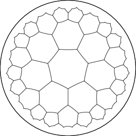
Figure 1: Regular heptagonal lattice established on the Poincaré disk. The number of concentric layers of heptagons is $L=3$ in this figure. All heptagons depicted within the circle are congruent with respect to the metric given in Eq. (3). The circumference corresponds to an infinite distance from the center of the circle.

The size of our lattice is characterized by the number of concentric layers of heptagons, denoted by $L$, which effectively functions as the linear dimension in our lattice. It is noteworthy that the total number of sites $N$ for our heptagonal lattices exhibit a complicated dependence on $L$ that is expressed as

$$N(1) = 7,$$

$$N(L) = 7+7\sum_{j=0}^{L-2}\left(u_{+}{v_{+}}^{j}+u_{-}{v_{-}}^{j}\right),\;[L\geq 2]$$ (4)

where $u_{\pm}$ and $v_{\pm}$ are defined by

$$u_{\pm}=2\pm\sqrt{5},\;\;\;v_{\pm}=\frac{1+u_{\pm}}{2}.$$ (5)

When $L\gg 1$, the total sites $N$ grows asymptotically as $N\propto e^{L}$, which is quite rapid in comparison with the case of the planar Ising model: $N\propto L^{2}$. This exponential increase in $N$ is a manifestation of the constant negative curvature of the underlying geometry, resulting in that the ratio $[N(L)-N(L-1)]/N(L)$ approaches a non-zero constant $1-e^{-1}$ in the limit $L\to\infty$. The latter feature means that the boundary sites of our lattices can not be neglected even in the thermodynamic limit, but contain a finite fraction of the total sites.

Boundary effects coming from these sites are difficult to be eliminated completely, because the periodic boundary conditions are hard to be employed to regular lattices assigned on a pseudosphere. Thereby, we have used the following manner in order to reduce the boundary effects on physical quantities of the system. Suppose that an Ising lattice consists of $L_{\rm out}$ concentric layers of heptagons. Then, for employing the STR method (see Sec. 3 for its details), we take into account only the Ising spins involved in the interior $L_{\rm in}$ layers ($L_{\rm in}\leq L_{\rm out}$) so as to reduce the contribution of the spins locating near the boundary. In actual calculations, $L_{\rm in}$ is varied from 4 to 6, and for each $L_{\rm in}$ the number of disregarded layers $\delta L\equiv L_{\rm out}-L_{\rm in}$ is systematically increased from 0 to 3. By examining the asymptotic behavior for large $\delta L$, we can deduce the bulk properties of the Ising lattice model embedded on the pseudosphere. Similar procedure has been employed thus far [25, 28] to extract the bulk critical properties of the negatively curved system.

3 Short-time relaxation method

Our aim is to investigate the dynamic critical behavior of the ferromagnetic Ising model defined on the heptagonal lattice. The Hamiltonian of the system is given by

$$H=-J\sum_{<i,j>}s_{i}s_{j},\quad s_{i}=\pm 1,$$ (6)

where $\langle i,j\rangle$ denotes a pair of nearest-neighbour sites and $J(>0)$ is the coupling strength between them. Hereafter, temperatures and energies are expressed in units of $J/k_{\rm B}$ and $J$, respectively.

In order to determine the dynamic critical exponent, we use the short-time relaxation (STR) method [18, 20, 21, 22]. This method enables neglecting equilibration, thereby avoiding computational burden significantly as compared to dynamical simulations in equilibrium. The basis of the STR method is the measurement of the quantity [18, 35]

$$Q(t)=\left\langle{\rm sgn}\left(\sum_{i=1}^{N}s_{i}(t)\right)\right\rangle,\;\;{\rm sgn}(x)=\left\{\begin{array}[]{rr}1&(x>0),\\ -1&(x<0),\end{array}\right.$$ (7)

which is obtained by the conventional MC procedure. Here, the time $t$ is measured in terms of one MC sweep, and the angular bracket indicates that the average is taken over different time sequences that begin from the same initial configuration. In actual simulations, the initial configuration is selected as $s_{i}=1$ for all sites, thereby yielding $Q(0)=1$. It then follows a monotonic decay with an increase in $t$, and finally $Q(\infty)=0$, since there is no preferred direction at equilibrium ($t\to\infty$).

A dynamic scaling hypothesis suggests that in the vicinity of the critical temperature $T_{c}$, the quantity $Q$ obeys the following scaling form:

$$Q(t,\epsilon,N)={\cal Q}\left(tN^{-\bar{z}},\epsilon N^{1/\mu}\right).$$ (8)

Here, $\bar{z}$ and $\mu$ are referred to as the dynamic and static critical exponent, respectively, for the Ising lattices on the pseudosphere (The physical meaning of these exponents will be given soon below). It is noted that $N$ instead of $L$ is employed in (8) as a scaling variable; this is a direct consequence of the exponential increase $N\propto e^{L}$ discussed in Sec. 2.

The dynamic exponent $\bar{z}$ is determined as follows. At the transition point $T=T_{c}$, $\epsilon=0$ so that the second argument $\epsilon N^{1/\mu}$ of the scaling function ${\cal Q}$ vanishes. This yields

$$\left.Q(t,N)\right|_{\epsilon=0}=f(x)$$ (9)

with the definition $x=tN^{-\bar{z}}$. Equation (9) states that, if we calculate $Q(t)$ by maintaining $T=T_{c}$ and plot the results against $x$ by selecting an appropriate value of $\bar{z}$, the curves of $Q(t)$ for different $N$s should collapse onto a single curve. Hence, the dynamical exponent $\bar{z}$ can be identified as the optimal fitting parameter for Eq. (9). We should note that the evaluation of $\bar{z}$ by the above procedure requires the knowledge of the value of $T_{c}$ beforehand; therefore, in actual calculations we use the numerical data of $T_{c}$ obtained from canonical Monte Carlo simulations for the same model [14].

Apart from the value of $\bar{z}$, the STR method enables us to determine the static critical exponent $\mu$. This is achieved by extracting the data $Q(t_{0})$ at the specific time $t=t_{0}$ for various $T$ and $N$. The time $t_{0}$ is defined such that parameter $a=t_{0}N^{-\bar{z}}$ with fixed $\bar{z}$ is invariant to the change in $N$. Under this condition, we obtain

$$\left.Q(\epsilon,N)\right|_{t=t_{0}}=g(y),$$ (10)

where $y$ is defined as $y=\epsilon N^{1/\mu}$. As a result, fitting the data of $Q(t_{0})$ for different $T$ and $N$ onto a single curve against $y$ yields the values of $\mu$ and $T_{c}$ as the optimal fitting parameters. This procedure provides a complementary method to determine $\mu$ and $T_{c}$, which were extracted in [14].

It deserves further comment about the exponents $\bar{z}$ and $\mu$ introduced in (8). From the scaling hypothesis, the exponent $\bar{z}$ is assumed to describe the dynamic scaling law

$$\tau\propto{\xi_{V}}^{\bar{z}}$$ (11)

between the relaxation time $\tau$ and the correlation volume $\xi_{V}$. Here, $\xi_{V}$ is a natural generalization [33, 36] of the localization length $\xi$, thus obeying the power law $\xi_{V}\propto\epsilon^{-\mu}$ in the vicinity of $T_{c}$. When the underlying geometry is a $d$-dimensional flat surface (or space), $\xi_{V}\propto\xi^{d}$ holds so that (11) yields $\bar{z}=z/d\sim 1.1$ for two-dimensional planar Ising models. However, when the underlying geometry is curved, the relation $\xi_{V}\propto\xi^{d}$ becomes invalid so that $\bar{z}$ may take a value different from the above. Similarly, the static exponent $\mu$ reduces to $\mu=\nu d=2$ for planar Ising models (because $\nu=1$ [38]), while it is not the case for curved cases. In fact, our numerical simulations have revealed that the dynamic exponent $\bar{z}$ for heptagonal Ising lattices exhibits a quantitative deviation from that for planar ones, as will be seen in the next section.

4 Results: Dynamic exponent $\bar{z}$

4.1 $\bar{z}$ for entire lattices $(\delta L=0)$

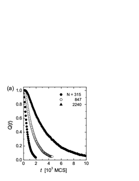
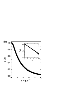
Figure 2: (a) Calculated results of $Q(t)$ for various lattice sizes $N$. (b) Finite size scaling of $Q(t,N)$ against the scaling variable $x=tN^{-\bar{z}}$. The critical temperature $T_{c}=1.25$ is assumed in accordance with Ref. [14]. The estimated value of $\bar{z}$ is $\bar{z}=0.90(2)$ with a 95% confidence interval. (c) The dependence of $\bar{z}$ on the number of disregarded layers $\delta L$. The solid line serves as a guide to eye.

Before addressing the bulk critical properties, we first demonstrate the results for entire heptagonal lattices with $\delta L=0$ (boundary contributions are fully involved). Figure 2 (a) shows the short-time relaxation behavior of $Q(t)$ for various systems sizes $N$. The temperature is fixed at $T=T_{c}=1.25$ consistent with Ref. [14], and the standard local update algorithm [37] is employed in order to calculate the time evolution of $Q(t)$. $N$ is varied from $315$ to $2240$; this corresponds to the change in the number of concentric layers from $L_{\rm in}=4$ to $L_{\rm in}=6$ (See Eq. (4)). For each value of $N$, we have performed a sample average for more than $3\times 10^{4}$ independent runs.

We see that all curves of $Q(t)$ in Fig. 2 (a) exhibit a monotonic decay from the initial value of $Q(0)=1$ toward the equilibrium value $Q(\infty)=0$. The decay time grows systematically with an increase in the system size $N$ as expected from the scaling law $\tau\propto N^{\bar{z}}$. Hence, rescaling the horizontal axis $t$ of Fig. 2 (a) by dividing it by the factor $N^{\bar{z}}$ with an appropriate exponent $\bar{z}$ yields the fitting of all curves into a single curve.

Figure 2 (b) presents the scaling attempt of $Q$ by taking $x\equiv tN^{-\bar{z}}$ as a scaling argument. The dynamic exponent $\bar{z}$ is determined as the optimal value that minimizes the following quantity [36]:

$$\Delta(\bar{z})=\sum_{i=1}^{n_{\rm seg}}\sum_{x\in X_{i}}\left[\frac{Q(x)-a_{i}-b_{i}x}{\sigma(x)}\right]^{2},$$ (12)

where $a_{i}$ and $b_{i}$ are fitting parameters, and $\sigma(x)$ is the standard deviation of $Q$. Note that in (12), the entire $x$ range is partitioned into $n_{\rm seg}$ segments $X_{i}$ with equal intervals. We have set $n_{\rm seg}=20$ in actual calculations, and extracted the values of $a_{i}$ and $b_{i}$ $(1\leq i\leq 20)$ that minimize $\Delta(\bar{z})$ for a given $\bar{z}$. By probing the behavior of $\Delta(\bar{z})$ with respect to $\bar{z}$, we have attained the optimal value $\bar{z}=0.90(2)$ with a 95% confidence interval. The resulting plot shown in Fig. 2 (b) displays the best collapse onto a single curve $f(x)$ in a broad range of the scaling variable $x=tN^{-\bar{z}}$. Importantly, the resulting value $\bar{z}\simeq 0.9$ is somewhat smaller than that of the planar Ising model $\bar{z}=z/d\simeq 1.1$. Since the boundary contribution is fully involved in the present case $(\delta L=0)$, the above deviation of $\bar{z}$ possibly stems from the mixture effect of the boundary Ising spins and the interior heptagonal Ising lattice.

4.2 $\bar{z}$ for bulk lattices $(\delta L\geq 1)$

We now turn to the study of bulk critical properties of the heptagonal Ising lattice model. As mentioned in Sec. 2, the boundary spins of Ising lattices on a pseudosphere are thought to affect significantly to the nature of the system; this is because the number of the spins along the boundary increases as fast as that of total spins of the lattice. Thereby, in order to extract the bulk critical exponents, we try to remove the boundary contribution by setting the disregarded layers $\delta L=L_{\rm out}-L_{\rm in}$ to be finite, i.e., by summing up only the spins within the interior $L_{\rm in}$ layers when performing MC simulations on the systems consisting of $L_{\rm out}(>L_{\rm in})$ layers.

The calculated results are summarized in Figure 2 (c); each data of $\bar{z}$ was extracted by the scaling analysis for lattices of $4\leq L_{\rm in}\leq 6$ and a given $\delta L$. The appropriate value of $T_{c}$ for each $\delta L$ is again referred to the results obtained from canonical MC simulations [14]. (Hence, the maximum system size we have treated reaches $L_{\rm out}=9$, which corresponds to $N=40432$.) We have observed that $\bar{z}$ monotonically decreases with increasing $\delta L$ within the range $0\leq\delta L\leq 3$. The monotonic decrease in $\bar{z}$ indicates that for sufficiently large $\delta L$, $\bar{z}$ takes a value that is considerably smaller than the corresponding value of the planar Ising models: $\bar{z}\simeq 1.1$. Thus, it follows that the bulk Ising lattices assigned on the negatively curved surfaces belong to a dynamic universality class distinct from those of the planar Ising models. The determination of the asymptotic value of $\bar{z}$ for $\delta L\gg 1$ would provide further conclusive information; this would require a huge computational effort. Instead, we have provided a concise argument regarding the asymptotic value of $\bar{z}$ in Section 6; this argument implies that the dynamic exponent in our system takes the mean-field exponent $\bar{z}_{\rm MF}=1/2$ in the limit $\delta L\to\infty$.

5 Results: Static critical exponent $\mu$

We now focus on the estimation of the static critical exponent $\mu$ and the critical temperature $T_{c}$ on the basis of the scaling relation (10). Figure 3 (a) presents the $T$-dependence of $Q(T)$ under the condition $\delta L=0$. Parameter $a=tN^{-z}$ is fixed at $a=1.5$, where $\bar{z}=0.90$ is set in accordance with the result from Fig. 2 (b). We observe a unique crossing point at $Q\simeq 0.74$ and $T\simeq 1.25$. Even when the values of parameter $a$ are varied, a crossing point still appears at a temperature almost identical to $T\simeq 1.25$, as expected from Eq. (8). Hence, it provides a rough estimate of the critical temperature $T_{c}$.

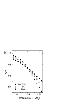
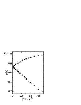
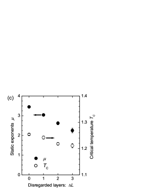
Figure 3: (a) Calculated results of $Q(T)$ for various values of $N$. Parameter $a=tN^{-\bar{z}}$ and the exponent $\bar{z}$ are fixed at $a=1.5$ and $\bar{z}=0.90$ for all values of $N$, respectively. (b) A scaling plot of $Q(T,N)$ against the scaling variable $y=\epsilon N^{1/\mu}$. The optimal values of $\mu$ for upper and lower branch are $\mu=3.45(4)$ and $\mu=3.36(3)$, respectively. The critical temperature is estimated as $T_{c}=1.254(3)$ for the two branches. (c) $\delta L$-dependences of $\mu$ and $T_{c}$.

The full scaling plot for $Q(T)$ is displayed in Fig. 3 (b). The fitting process was based on a polynomial expansion of the scaling function $g(y)$ expressed in Eq. (10) as

$$g(y)\simeq\sum_{j=0}^{3}c_{j}\left(\epsilon N^{1/\mu}\right)^{j},$$ (13)

where $c_{j}$, $T_{c}$, and $\mu$ are considered as fitting parameters. A very smooth collapse is obtained with $\mu=3.45(4)$ for the upper branch, and $\mu=3.36(3)$ for the lower one. The critical temperature is estimated as $T_{c}=1.254(3)$ for both branches. It was also confirmed that the values of $\mu$ and $T_{c}$ are almost invariant to the change in the value of parameter $a$ that is arbitrarily chosen within the range of $0.5\leq a\leq 3.0$.

We have then clarified the boundary contribution to the values of $\mu$ and $T_{c}$ by setting $\delta L\geq 1$. Figure 3 (c) shows the $\delta L$-dependence of $\nu$ and $T_{c}$ under the same numerical conditions with respect to $L_{\rm in}$ and $a$ as in the case of $\delta L=0$. It is found that both $\mu$ and $T_{c}$ decreases monotonically with increasing $\delta L$. Further noteworthy is the fact that all the values of $\mu$ and $T_{c}$ given in Fig. 3 (c) are in excellent agreement with those obtained by MC simulations in equilibrium [14], where the tendency of $\mu$ toward the mean field exponent $\mu_{\rm MF}=2$ in the limit $\delta L\to\infty$ has been suggested. This consistency with respect to $\mu$ and $T_{c}$ strongly supports the validity of our STR approach to the critical behavior of the Ising model on curved surfaces.

6 Discussions

It has been demonstrated that the dynamic critical exponent $\bar{z}$ of the heptagonal Ising lattice model exhibit a quantitative deviation from that of the planar Ising model $\bar{z}\simeq 1.1$. In fact, it takes a value $\simeq 0.9$ under the condition $\delta L=0$, and still continues to decrease almost linearly with $\delta L$. This behavior of $\bar{z}$ indicates the occurrence of a novel universality class with regard to dynamic criticality, and evidences the conjecture that the peculiar intrinsic geometry of the underlying surface affects the dynamic critical properties of the embedded system. Besides, the static critical exponent $\mu$ also turns out to exhibit a monotonic decrease with increasing $\delta L$ toward a particular value of $\mu_{\rm MF}=2$, which is consistent with the value derived from the mean field theory.

The mean field behavior of $\mu$ has been suggested earlier by Rietman et al. [25] and by Doyon and Fonseca [28]. This behavior is attributed to the fact that an Ising lattice embedded on a pseudosphere is effectively an infinite dimensional lattice at large distance due to the exponential growth of the total spins $N$ [39]. For an ordinary Ising lattice in $d$ dimension, the number of spins along the boundary, $N_{s}$, is expressed by $N_{s}\propto N^{1-(1/d)}$. Hence, by comparing it with the peculiar relation $N_{s}\propto N$ that is valid on negatively curved surfaces, we eventually reach the consequence $d=\infty$ for the latter geometry. As a result, our heptagonal Ising lattices yield the mean-field critical exponent $\mu_{\rm MF}=\nu_{\rm MF}d_{c}=2$ [33], where $\nu_{\rm MF}=1/2$ is the mean-field exponent and $d_{c}=4$ is the upper critical dimension for the Ising model.

In this context, the dynamic critical exponent $\bar{z}$ on negatively curved systems is supposed to exhibit the mean field exponent $\bar{z}_{\rm MF}=z_{\rm MF}/d_{c}=1/2$ at $\delta L\gg 1$, since $z_{\rm MF}=2$ for the Ising model. This inference is indeed consistent with our numerical results; as shown in Fig. 2 (c), $\bar{z}$ takes a smaller value than the planar case ($\bar{z}\sim 1.1$) whatever value $\delta L$ is, and moreover, it monotonically decreases with reducing the boundary contribution up to $\delta L=3$. Hence, when extrapolated to the bulk limit $\delta L\gg 1$, it yields the mean field exponent $\bar{z}_{\rm MF}=1/2$ as similar to the case of static critical exponents [14]. We also note that it is interesting to investigate the dynamics exponents associated with the Griffiths-type phase transition in the Ising model defined on negatively curved surfaces [27]; a comparison between the dynamics exponent of the bulk region and that of the boundary region will provide a better understanding of the critical dynamics of entire Ising lattices defined on negatively curved surfaces.

Further noteworthy is that the surface curvature effect on critical properties of the assigned spin lattice model would become richer if the spin variables possess orientational degrees of freedom. In the latter cases, the interacting energy of neighboring spins is determined by their relative angle, which is a function of a spatially-dependent metric tensor. Thereby, the Hamiltonian of the system involves the metric tensor in an explicit form. As a result, the energetically preferable spin configurations and the temporal fluctuations of the order parameters are directly influenced by the intrinsic geometry of the surface determined by the metric tensor. It is thus expected that these vector-spin models defined on curved surfaces exhibit peculiarities associated with phase transition and low energy excitations [40, 41, 42, 43, 44]. To the best of our knowledge, there was no attempt to reveal the dynamic critical exponent of vector-spin lattice models defined on curved surfaces. The STR method that we have utilized is applicable to these systems; detailed analyses of this issue will be presented in future.

7 Conclusion

In the present study, we have investigated the dynamic critical behavior of the regular heptagonal Ising model defined on a curved surface with constant negative curvature. The STR methods that incorporate finite-size scaling analyses have been employed in order to compute the dynamical critical exponent $\bar{z}$ as well as the static critical exponent $\mu$ for the correlation volume $\xi_{V}$. The resulting values of both the exponents are distinct from those of the planar Ising model. Furthermore, we have studied quantitatively how the boundary spins contribute to the determination of $\bar{z}$ and $\mu$, and eventually we have revealed that they both reduce to the mean field exponent $\bar{z}_{\rm MF}=1/2$ and $\mu_{\rm MF}=2$ in the bulk limit. We hope that our results prove to be a fundamental basis for further fruitful studies on the critical behaviors occurring on curved surfaces.

Appendix A The Gaussian curvature in the Poincaré disk

This appendix demonstrates that the Poincaré disk possesses the negative constant value $\kappa=-1$ at an arbitrary point within the disk. The Gaussian curvature $\kappa$ at a given position is defined by [45]

$$\kappa\equiv-R/2,$$ (14)

with the quantities:

$$R\equiv g^{ij}R_{ij},\;\;R_{ij}\equiv g^{kl}R_{kilj}.$$ (15)

Here, $R$, $R_{ij}$, and $R_{kilj}$ are termed as the scalar curvature, Ricci tensor, and curvature tensor, respectively. (Hereafter, we will use the summation convention on repeated indices.) The $g^{ij}$ is the inverse of the metric tensor $g_{ij}$ that determines the line element at a given position as $ds^{2}=g_{ij}dx^{i}dx^{j}$. Note that all the three quantities $R$, $R_{ij}$, and $R_{kilj}$ are functions of $g_{ij}$. Hence, in principle, the knowledge of $g_{ij}$ and the explicit form of $R_{kilj}$ are sufficient to calculate the value of $\kappa$, while the actual calculations are lengthy as shown below.

The explicit dependence of the curvature tensor $R_{kilj}$ on $g_{ij}$ is expressed as:

$$R_{kilj} = g_{km}R^{m}_{\;\;ilj},$$ (16)

$$R^{m}_{\;\;ilj} = \partial_{l}{\it\Gamma}^{m}_{\;\;ij}-\partial_{j}{\it\Gamma}^{m}_{\;\;il}+{\it\Gamma}^{m}_{\;\;pl}{\it\Gamma}^{p}_{\;\;ij}-{\it\Gamma}^{m}_{\;\;pj}{\it\Gamma}^{p}_{\;\;il},\;\;\;$$ (17)

where ${\it\Gamma}^{m}_{\;\;ij}$ is the connection defined by

$${\it\Gamma}^{m}_{\;\;ij}=\frac{g^{mp}}{2}\left(\partial_{j}g_{pi}+\partial_{i}g_{pj}-\partial_{p}g_{ij}\right).$$ (18)

Equations (16)–(18) yield an alternative form of $R_{kilj}$, which is expressed as:

$$R_{kilj} = \frac{1}{2}\left(\partial_{i}\partial_{j}g_{kl}+\partial_{k}\partial_{l}g_{ij}-\partial_{k}\partial_{j}g_{il}-\partial_{i}\partial_{l}g_{kj}\right)$$ (19)

$$+\;g_{rs}\left({\it\Gamma}^{r}_{\;lk}{\it\Gamma}^{s}_{\;ij}-{\it\Gamma}^{r}_{\;jk}{\it\Gamma}^{s}_{\;il}\right).$$

It is noteworthy that due to the symmetric property of Eq. (19), the tensor $R_{kilj}$ has only four non-zero components in a two dimensional system. Further, these components are related to each other in the following manner:

$$R_{1212}=\;-R_{2112}=\;-R_{1221}=R_{2121}.$$ (20)

As a result, the tensor $R_{kilj}$ is determined by only a single component $R_{1212}$. In addition, the symmetric property of $R_{kilj}$ results in the following equality with respect to the components of the Ricci tensor $R_{ij}$:

$$R_{11}=g^{22}R_{2121},\;\;R_{22}=g^{11}R_{1212},$$ (21)

and $R_{12}=R_{21}=0$. Consequently, we can represent the scalar curvature $R$ in two-dimensional systems as

$$R = g^{11}R_{11}+g^{22}R_{22}$$ (22)

$$= g^{11}g^{22}R_{2121}+g^{22}g^{11}R_{1212}$$

$$= \frac{2R_{1212}}{g},$$

where $g={\rm det}[g_{ij}]$, and thus $g^{11}=g_{22}/g$ and $g^{22}=g_{11}/g$. Equation (22) yields the key relation between the component $R_{2121}$ and the Gaussian curvature $\kappa$ as follows:

$$\kappa=-\frac{R_{1212}}{g}.$$ (23)

This identity is known to hold for general two-dimensional systems [45].

The value of $R_{1212}$ for our model is evaluated by the following procedure. For the Poincaré disk, the metric tensor $g_{ij}$ is represented in the matrix form as follows:

$$\left[g_{ij}\right]=\left(\begin{array}[]{cc}4f&\;0\\[5.69054pt] 0&\;4r^{2}f\end{array}\right),\;\;\;f\equiv\frac{1}{(1-r^{2})^{2}}.$$ (24)

This means that the line element on the Poincaré disk is given by $ds^{2}=4f(dr^{2}+r^{2}d\theta^{2})$, as already shown in Eq. (3). Straightforward calculation based on the metric (24) reveals that there are four non-zero components of the Christoffel symbol ${\it\Gamma}^{m}_{\;\;ij}$ expressed as

$${\it\Gamma}^{1}_{\;\;11} = \frac{g^{11}}{2}\partial_{1}g_{11},\quad{\it\Gamma}^{1}_{\;\;22}=-\frac{g^{11}}{2}\partial_{1}g_{22},$$

$${\it\Gamma}^{2}_{\;\;12} = {\it\Gamma}^{2}_{\;\;21}=\frac{g^{22}}{2}\partial_{1}g_{22}.$$ (25)

By substituting Eqs. (24) and (25) into the expression of the tensor $R_{kilj}$ (19), we directly obtain:

$$R_{1212}=\frac{16r^{2}}{(1-r^{2})^{4}}\;=\;\frac{1}{g}.$$ (26)

Eventually, by comparing it with Eq. (23), we arrive at the final conclusion $\kappa=-1$ for arbitrary positions within the Poincaré disk.

References

References

- [1] Kazakov V A 1986 Phys. Lett. A 119 140
- [2] Crnkovic C, Ginparg P and Moore G 1990 Phys. Lett. B 237 196
- [3] Gross M and Harber H W 1991 Nucl. Phys. B 364 703
- [4] Francesco P Di, Ginsparg P and Zinn-Justin J 1995 Phys. Rep. 254 1
- [5] Holm C and Janke W 1996 Phys. Lett. B 375 69
- [6] Himpsel F J, Ortega J E, Mankey G J and Willis R F 1998 Adv. Phys. 47 511
- [7] Martín J I, Nogués J, Liu K, Vicente J L, and Schuller I K 2003 J. Magn. Magn. Mater. 256 449
- [8] Diego O, Gonzalez J and Salas J 1994 J. Phys. A: Math. Gen. 27 2965
- [9] Hoelbling Ch and Lang C B 1996 Phys. Rev. B 54 3434
- [10] González J 2000 Phys. Rev. E 61 3384
- [11] Weigel M and Janke W 2000 Europhys. Lett. 51 578
- [12] Costa-Santos R 2003 Phys. Rev. B 68 224423; 2003 Acta. Phys. Pol. B 34 4777
- [13] Pleimling M 2004 J. Phys. A 37 R79
- [14] Shima H and Sakaniwa Y 2006 J. Phys. A 39 4921
- [15] Cardy J, 1996 Scaling and Renormalization in Satistical Physics (Cambridge University Press, Cambridge UK)
- [16] Calabrese P and Gambassi A 2005 J. Phys. A 38 R133
- [17] Nightingale M P and Blöte H W J 1996 Phys. Rev. Lett. 76 4548
- [18] Soares M S, daSilva J K L and Barreto F C S 1997 Phys. Rev. B 55 1021
- [19] Nightingale M P and Blöte H W J 2000 Phys. Rev. B 62 1089
- [20] Li Z B, Schülke L and Zhang B 1995 Phys. Rev. Lett. 74 3396
- [21] Janssen H K, Schaub B and Schmittmann B 1989 Z. Phys. B 73 539
- [22] Zheng B 1998 Int. J. Mod. Phys. B 12 1419
- [23] Coxeter H S M 1969 Introduction to Geometry (Wiley, New York)
- [24] Firby P A and Gardiner C F 1991 Surface Topology (Ellis Horwood, London)
- [25] Rietman R, Nienhuis B and Oitmaa J 1992 J. Phys. A: Math. Gen. 25 6577
- [26] Elser V and Zeng C 1993 Phys. Rev. B 48 13647
- [27] d’Auriac J C A, Mélin R, Chandra P and Douçot B 2001 J. Phys. A: Math. Gen. 34 675
- [28] Doyon B and Fonseca P 2004 J. Stat. Mech. P07002
- [29] Balazs N L and Voros A 1986 Phys. Rep. 143 109
- [30] Avron J E, Klein M, Pnueli A and Sadun L 1992 Phys. Rev. Lett. 69 128
- [31] D’Hoker E and Phong D H 1988 Rev. Mod. Phys. 60 917
- [32] Levin J 2002 Phys. Rep. 365 251
- [33] Botet R, Jullien R and Pfeuty P 1982 Phys. Rev. Lett. 49 478
- [34] Das P K and Sen P 2005 Eur. Phys. J. B 47 391
- [35] deOliveira P M C 1992 Europhys. Lett. 20 621
- [36] Medvedyeva K, Holme P, Minnhagen P, and Kim B J 2003 Phys. Rev. E 67 036118
- [37] Binder K and Heermann D W 2002 Monte Carlo simulation in Statistical Physics, (Springer)
- [38] Kaufman B and Onsager L 1949 Phys. Rev. 76 1244
- [39] Callan C and Wilczek F 1990 Nucl. Phys. B 340 366
- [40] Saxena A and Dandoloff R 1997 Phys. Rev. B 55 11049
- [41] Balakrishnan R and Saxena A 1998 Phys. Rev. B 58 14383
- [42] Freitas W A, Moura-Melo W A and Pereira A R 2005 Phys. Lett. A 336 412
- [43] Pereira A R 2005 J. Magn. Magn. Mater. 285 60
- [44] Moura-Melo W A, Pereira A R, Mól L A S and Pires A S T 2006 Phys. Lett. A in press; cond-mat/0511443
- [45] Landau L D and Lifshitz E M 1980 The Classical Theory of Fields (Butterworth-Heinemann)