Transport of Dirac quasiparticles in graphene: Hall and optical conductivities

Abstract

The analytical expressions for both diagonal and off-diagonal ac and dc conductivities of graphene placed in an external magnetic field are derived. These conductivities exhibit rather unusual behavior as functions of frequency, chemical potential and applied field which is caused by the fact that the quasiparticle excitations in graphene are Dirac-like. One of the most striking effects observed in graphene is the odd integer quantum Hall effect. We argue that it is caused by the anomalous properties of the Dirac quasiparticles from the lowest Landau level. Other quantities such as Hall angle and Nernst signal also exhibit rather unusual behavior, in particular when there is an excitonic gap in the spectrum of the Dirac quasiparticle excitations.

I Introduction

There is significant progress in fabrication of free-standing monocrystalline graphite films with thickness down to a single atomic layer Novoselov2004Science ; Novoselov2005PNAS and the relatively thick (thicker than 3 monolayers) graphite films Berger2004JPCB ; Zhang2005PRL ; Bunch2005Nano ; Morozov2005 are now widely produced. The new one layer material, called graphene, possesses truly remarkable properties both from a technological and theoretical point of view. Graphene is a promising candidate for applications in future micro- and nanoelectronics due to its excellent mechanical characteristics, scalability to the nanometer sizes, and the ability to sustain huge ($>10^{8}A/cm^{2}$) electric currents. By using the electric field effect Novoselov2004Science ; Novoselov2005PNAS ; Zhang2005PRL ; Bunch2005Nano ; Morozov2005 ; Geim-new ; Kim-new , it is possible to change the carrier concentration in samples by tens times and even to change the carrier type from electron to hole when the sign of applied gate voltage is reversed. Another interest in graphene is related to the fact that it represents a building block for the other forms of carbon, viz. graphite is a stack of graphene layers, carbon nanotubes are wrapped graphene layers, while fullerenes can be created from graphene by introducing topological defects.

On the theoretical side, the conduction and valence bands in graphene touch upon each other at isolated points in the Brillouin zone and this results in the linear, Dirac-like (up to energies of the order of $1000$ K) spectrum of quasiparticle excitations which makes graphene a unique truly two-dimensional ”relativistic” electronic system. The thinnest graphite films can be described by a low-energy (2+1) dimensional effective massless Dirac theory Semenoff1984PRL ; Gonzales1993NP . A recent observation Geim-new ; Kim-new of the unconventional integer quantum Hall effect (IQHE)

$$\sigma_{xy}=-\frac{2e^{2}}{h}(2n+1),\qquad n=0,1,\ldots$$ (1)

which is expected from the analytical study Gusynin2005PRL based on the fundamental properties of the $2+1$ dimensional Dirac theory, can be considered as the ultimate proof of the existence of the Dirac quasiparticles in this fascinating material. A complementary numerical investigation of the Landau level structure for a hexagonal lattice model with the nearest neighbor and next-nearest neighbor hoppings also led the authors of Ref. Peres2005 to the conclusion that the Hall conductivity is quantized according to the rule (1). In contrast to this behavior expected for an ideal 2D graphene, thicker 2 to 10 layers thick films studied in Refs. Novoselov2004Science ; Novoselov2005PNAS ; Berger2004JPCB exhibit instead a conventional Hall quantization $\sigma_{xy}=-4(e^{2}/h)n$.

The Dirac quasiparticles seem to be present not only in graphene, but also in the highly oriented pyrolitic graphite (HOPG), single crystalline Kish graphite and the relatively thick (thicker than 3-10 monolayers) graphite films, where warping introduces other types of carriers Dresselhaus1974PRB . The Hall effect features in HOPG graphite were observed in Refs. Uji1998PB ; Kopelevich2003PRL (see also the latest Ref. Kempa2006SSC ), but the Hall conductivity quantization in these systems remains conventional Novoselov2004Science ; Berger2004JPCB ; Ocana2003PRB ; Kopelevich2003PRL . Nevertheless, the presence of the Dirac quasiparticles can be detected using other experimental techniques. For example, the differences between the Dirac and Schrödinger (massive) quasiparticles may be observed in thermodynamic and magnetotransport measurements Novoselov2004Science ; Ocana2003PRB ; Kopelevich2003PRL ; Berger2004JPCB ; Zhang2005PRL ; Bunch2005Nano ; Morozov2005 . For instance, the phase of de Haas van Alphen and Shubnikov de Haas oscillations for Dirac quasiparticles is shifted by $\pi$ Sharapov2004PRB ; Gusynin2005PRB ; Luk'yanchuk2004PRL ; Geim-new ; Kim-new compared to the phase of non-relativistic quasiparticles. Moreover, the Dingle and temperature factors in the amplitude of oscillations explicitly depend on the carrier density in the case of a Dirac-like spectrum Sharapov2004PRB ; Gusynin2005PRB . These two characteristic features allow one to distinguish the Dirac quasiparticles from very light, $\sim 0.01m_{e}$ ($m_{e}$ is the electron mass) particles, and from other carriers which are also present in graphite Luk'yanchuk2004PRL . The Landau levels in graphite are observed in high magnetic field using both scanning tunneling spectroscopy Matsui2005PRL and infrared spectroscopy Li2005 . The latter allowed one to observe in HOPG the cyclotron resonance modes and to establish that some of them reveal a $\sqrt{B}$ dependence of the cyclotron frequency which is expected for the Dirac quasiparticles. Actually, this characteristic, $\sqrt{B}$, dependence shows up in various properties related to the Dirac quasiparticles. An interesting example is the magnetization $M\sim-\sqrt{B}$ (cf. Eq. (7.4) of Ref. Sharapov2004PRB ) at zero chemical potential $\mu$ which implies that the magnetic susceptibility $\chi=\partial M/\partial B\varpropto-B^{-1/2}$ diverges at zero field. Although the singularity of $\chi(B\to 0)$ is smoothed [see Ref. Nersesyan1989JLTP , where another system with Dirac quasiparticles is considered] by a coupling between layers, finite temperature and/or chemical potential, the presence of Dirac quasiparticles results in an anomalously strong diamagnetism of graphite Beaugnon1991Nature .

The purpose of the present work is to extend the analysis made in the previous papers Gorbar2002PRB ; Sharapov2004PRB ; Gusynin2005PRB (see also Ref. Sharapov2003PRB devoted to a so called $d$-density wave state which is also described by the same low-energy Dirac Lagrangian) where thermodynamic and mostly diagonal dc magnetotransport properties of graphene were studied. We derive analytical expressions both for diagonal and off-diagonal ac conductivity which in contrast to the previous papers include a frequency dependent impurity scattering rate. Then we concentrate mostly on the dc Hall conductivity giving throughout derivations of the results presented in our short paper Ref. Gusynin2005PRL and considering the limiting cases that were not yet considered.

The paper is organized as follows. In Sec. II general features of the model for a single layer of graphene are described. In Sec. III we present the analytical expressions for both diagonal and off-diagonal ac conductivities, including dc limits of these expressions (the details of calculation are given in Appendix A). Then in Sec. IV we consider the dc Hall conductivity, the Hall angle and the Nernst signal are studied in Sec. V. In particular in Sec. V.2 we discuss a possibility of detecting a gap that may exist in the spectrum of the quasiparticle excitations of graphene. In Conclusions, Sec. VI we give a concise summary of the obtained results. The extra technical details concerning the Hall conductivity in the clean limit are given in Appendix B. The equation for chemical potential $\mu$ is considered in Appendix C and the solution of the Dirac equation in the symmetric gauge is presented in Appendix D.

II Model

As discussed, for example, in Refs. Gorbar2002PRB ; Sharapov2004PRB ; Gusynin2005PRB , we start directly from the conventional QED₂₊₁ Lagrangian density

$$\mathcal{L}=\sum_{\sigma=\pm 1}\bar{\Psi}_{\sigma}(t,\mathbf{r})\left[i\gamma^{0}(\hbar\partial_{t}-i\mu_{\sigma})+iv_{F}\gamma^{1}\left(\hbar\partial_{x}+i\frac{e}{c}A_{x}^{\mathrm{ext}}\right)+iv_{F}\gamma^{2}\left(\hbar\partial_{y}+i\frac{e}{c}A_{y}^{\mathrm{ext}}\right)-\Delta\right]\Psi_{\sigma}(t,\mathbf{r}),$$ (2)

where $\Psi_{\sigma}=(\psi_{1\sigma}(t,\mathbf{r}),\psi_{2\sigma}(t,\mathbf{r}))$ is the four-component Dirac spinor combined from two spinors $\psi_{1\sigma},\psi_{2\sigma}$ [corresponding to $\mathbf{K}$ and $\mathbf{K}^{\prime}$ points of the Fermi surface, respectively] that describe the Bloch states residing on the two different sublattices of the biparticle hexagonal lattice of the graphene sheet. In Eq. (2) $\gamma^{\nu}$ with $\nu=0,1,2$ are $4\times 4$ $\gamma$ matrices belonging to a reducible representation in $2+1$, for example, $\gamma^{\nu}=\sigma_{3}\otimes(\sigma_{3},i\sigma_{2},-i\sigma_{1})$, $\bar{\Psi}_{\sigma}=\Psi_{\sigma}^{\dagger}\gamma^{0}$ is the Dirac conjugated spinor, $-e<0$ is the electron charge, $v_{F}$ is the Fermi velocity, and $\sigma=\pm 1$ is the spin variable. More generally the number of spin components $N_{f}$ can be regarded as a flavor index and $N_{f}=2$ corresponds to the physical case.

The external magnetic field $\mathbf{B}=\nabla\times\mathbf{A}^{\mathrm{ext}}$ is applied perpendicular to the plane along the positive z axis and the corresponding vector potential is taken in the symmetric gauge $\mathbf{A}^{\mathrm{ext}}=(-By/2,Bx/2)$. The energy scale associated with the magnetic field expressed in the units of temperature reads

$$\frac{eBv_{F}^{2}}{c}\to\frac{eB\hbar v_{F}^{2}}{c}\frac{1}{k_{B}^{2}}(K^{2})=8.85\times 10^{-8}v_{F}^{2}(\mbox{m/s})B(T),$$ (3)

where $v_{F}$ and $B$ are given in m/s and Tesla, respectively. In the following we set $\hbar=k_{B}=1$, and in some places $e=c=1$, unless stated explicitly otherwise. There is some disagreement in the literature concerning the precise value of $v_{F}$ in graphene which is related to an uncertainty in the value of the nearest-neighbor hopping $t$. For numerical calculations we assume that $t\sim 2.3\mbox{eV}$, so that $v_{F}\approx 7.4\times 10^{5}\mbox{m/s}$ which leads to the relationship $eB\to(4.85\times 10^{4}\mbox{K}^{2})B(\mbox{T})$. Note that the latest experiments Geim-new ; Kim-new indicate that $v_{F}\approx(1\div 1.1)\times 10^{6}\mbox{m/s}$.

Since the Lagrangian (2) originates from a nonrelativistic many-body theory, the Zeeman interaction term has to be explicitly included by considering spin splitting $\mu_{\sigma}=\mu-\sigma g/2\mu_{B}B$ of the chemical potential $\mu$, where $\mu_{B}=e\hbar/(2mc)$ is the Bohr magneton and $g$ is the Lande factor. However, for the relativistic quasiparticle spectrum with the realistic values of $v_{F}\varpropto 10^{6}\mbox{m/s}$ and $g\sim 2$ the distance between Landau levels turns out to be very large compared to the Zeeman splitting Gusynin2005PRB , so that in what follows we will not consider this term and just multiply all relevant expressions by the above-mentioned number of flavors $N_{f}$. We note, however, that the latest measurements in high fields (up to $45\mbox{T}$) Zhang2006 revealed a lifting of the spin and sublattice degeneracy, so that the half integer Hall quantization changes to the integer one for fields $B>20\mbox{T}$.

While simple tight-binding calculations (see e.g. Ref. Saito.book ) made for hexagonal lattice of a single graphene sheet predict that $\mu=0$, the real picture is more complicated and the actual value of $\mu$ in HOPG is nonzero due to inter-layer hopping, finite doping, and/or disorder. Moreover, a nonzero and even tunable value of $\mu$ (including the change of the character of carriers, either electron or holes) is possible in the electric-field doping experiments made on monocrystalline graphitic films Novoselov2004Science ; Novoselov2005PNAS ; Zhang2005PRL ; Bunch2005Nano ; Geim-new ; Kim-new ; Morozov2005 . In our notations $\mu>0$ corresponds to electrons and, accordingly, to the positive gate voltage, $V_{g}$.

The Lagrangian (2) also includes a gap $\Delta$, so that for $B=0$ it describes quasiparticles with the dispersion $E(\mathbf{k})=-\mu\pm\sqrt{v_{F}^{2}\mathbf{k}^{2}+\Delta^{2}}$. Again, this gap is zero when non-interacting quasiparticles on the hexagonal lattice with nearest neighbor hopping are considered. However, it could open as a result of poor screening of the Coulomb interaction in graphite Khveshchenko2001PRL ; Gorbar2002PRB and/or in the presence of an external magnetic field (the phenomenon of magnetic catalysis) Gusynin1995PRD . The physical meaning of this gap (or a singlet excitonic order parameter) is directly related to the electron density imbalance between the A and B sublattices of the bi-particle hexagonal lattice of graphene Khveshchenko2001PRL . The opening of such a gap was already the subject of an experimental investigation Kopelevich2003PRL and we hope that the predictions made in Refs. Khveshchenko2001PRL ; Gorbar2002PRB will be tested again on the new thin samples that are closer to the ideal graphene considered in these theoretical papers.

In contrast to the diagonal transport coefficients, the off-diagonal transport properties are sensitive to the sign of the product $eB$. Thus for the lucidity of the presentation, we begin with the expression for the spectral function of Dirac fermions and perform the calculation without assuming the positiveness of the product $eB$.

The Green’s function of Dirac fermions described by the Lagrangian (2) in an external field reads

$$S(t-t^{\prime},\mathbf{r};\mathbf{r}^{\prime})=\exp\left(-\frac{ie}{c}\mathbf{r}\mathbf{A}^{ext}(\mathbf{r^{\prime}})\right)\tilde{S}(t-t^{\prime},\mathbf{r}-\mathbf{r}^{\prime}),$$ (4)

where $\tilde{S}(t-t^{\prime},\mathbf{r}-\mathbf{r}^{\prime})$ is the translation invariant part of $S(t-t^{\prime},\mathbf{r}-\mathbf{r}^{\prime})$. Its derivation using the Schwinger proper-time method and decomposition over Landau level poles has been discussed in many papers (see, e.g. Refs. Gusynin1995PRD ; Chodos1990PRD ; Sharapov2003PRB ), so here we begin with the Fourier transform of ${\tilde{S}}(x-y)$ in the Matsubara representation

$$S(i\omega_{m},\mathbf{k})=e^{-\frac{c{\mathbf{k}}^{2}}{|eB|}}\sum\limits_{n=0}^{\infty}(-1)^{n}\frac{S_{n}(i\omega_{m},\mathbf{k})}{(i\omega_{m})^{2}-M_{n}^{2}},\qquad\omega_{m}=\pi(2m+1)T,$$ (5)

where $T$ is the temperature,

$$M_{n}=\sqrt{\Delta^{2}+2nv_{F}^{2}|eB|/c}$$ (6)

are the energies of the relativistic Landau levels and

$$S_{n}(i\omega_{m},\mathbf{k})=2(i\omega_{m}\gamma^{0}+\Delta)\left[P_{-}L_{n}\left(\frac{2c\mathbf{k}^{2}}{|eB|}\right)-P_{+}L_{n-1}\left(\frac{2c\mathbf{k}^{2}}{|eB|}\right)\right]-4\mathbf{k}{\boldsymbol{\gamma}}L_{n-1}^{1}\left(\frac{2c\mathbf{k}^{2}}{|eB|}\right),$$ (7)

with $P_{\pm}=(1\pm i\gamma^{1}\gamma^{2}{\rm sgn}(eB))/2$ being projectors and $L^{\alpha}_{n}(z)$ the generalized Laguerre polynomials. By definition, $L_{n}(z)\equiv L^{0}_{n}(z)$ and $L^{\alpha}_{-1}(z)\equiv 0$.

In what follows we also need the retarded and advanced Green’s functions that are obtained by analytic continuation from positive and negative discrete frequencies, respectively, $S^{R}(\omega+i0,\mathbf{k})=S(i\omega_{m}\to\omega+i0,\mathbf{k})$ and $S^{A}(\omega-i0,\mathbf{k})=S(i\omega_{m}\to\omega-i0,\mathbf{k})$. When the frequency dependent scattering rate $\Gamma(\omega)$ is included, they acquire the form

$$S^{(R,A)}(\omega,\mathbf{k})=e^{-\frac{c{\mathbf{k}}^{2}}{|eB|}}\sum\limits_{n=0}^{\infty}(-1)^{n}\frac{S_{n}^{(R,A)}(\omega\pm i\Gamma(\omega),\mathbf{k})}{(\omega\pm i\Gamma(\omega))^{2}-M_{n}^{2}}.$$ (8)

The scattering rate $\Gamma(\omega)$ is expressed via the retarded fermion self-energy, $\Gamma(\omega)=-{\rm Im}\Sigma^{R}(\omega)$ which in general depends on the energy, temperature, field and the Landau levels index $n$. This self-energy has to be determined self-consistently from the Schwinger-Dyson equation. The exact form of this equation actually depends on the model assumptions about the impurity scattering, e.g. whether the impurity scatterers are short- or long-range and in many cases this equation is solved numerically. Exactly this kind of consideration was made for graphene in Ref. Zheng2002PRB , but in our paper we pursue another goal which is to obtain a simple analytical expression for the Hall conductivity. Accordingly here we chose a different strategy. In Sec. III we derive general expressions for both frequency dependent $\sigma_{xx}(\Omega)$ and $\sigma_{xy}(\Omega)$ which include an unspecified frequency dependent scattering rate $\Gamma(\omega)$. However, we make an essential for the analytical work simplifying assumption that $\Gamma(\omega)$ is independent of the Landau levels index $n$. This assumption is justified when point-like impurity scattering is considered Champel2002PRB . The expressions obtained for $\sigma_{xx}(\Omega)$ and $\sigma_{xy}(\Omega)$ are suitable for investigation of microwave and optical conductivities in graphene. Then in Sec. IV we consider the case of constant width $\Gamma=\Gamma(\omega=0)=-{\rm Im}\Sigma^{R}(\omega=0)=1/(2\tau)$, where $\tau$ is the mean free time of quasiparticles and treat $\Gamma$ as a phenomenological parameter. This approximation allows one to obtain rather simple expressions for the Hall conductivity in the various limits.

III General representation for electrical conductivity

The frequency dependent electrical conductivity tensor is calculated using the Kubo formula

$$\sigma_{ij}(\Omega)=\frac{{\rm Im}\Pi^{R}_{ij}(\Omega+i0)}{\Omega},$$ (9)

where $\Pi^{R}_{ij}(\Omega)$ is the retarded current-current correlation function obtained by analytical continuation ($\Pi^{R}_{ij}(\Omega)=\Pi_{ij}(i\Omega_{m}\to\Omega+i0)$) of the imaginary time expression:

$$\Pi_{ij}(i\Omega_{m})=\frac{1}{V}\int\limits_{0}^{\beta}d\tau e^{i\Omega_{m}\tau}\langle T_{\tau}J_{i}(\tau)J_{j}(0)\rangle,\quad J_{i}(\tau)=\int d^{2}rj^{i}(\tau,\mathbf{r}),\quad\Omega_{m}=2\pi mT.$$ (10)

Here $V$ is the volume of the system, $\beta=1/T$ is the inverse temperature, and $j^{i}(\tau,\mathbf{r})$ is the electric current density operator

$$j^{i}(\tau,\mathbf{r})=-\frac{\delta\mathcal{L}}{\delta A_{i}}=-ev_{F}\sum_{\sigma}\bar{\Psi}_{\sigma}(\tau,\mathbf{r})\gamma^{i}\Psi_{\sigma}(\tau,\mathbf{r}).$$ (11)

The brackets in Eq. (10) denote the averaging in the grand canonical ensemble. Neglecting the impurity vertex corrections, the calculation of the conductivity reduces to the evaluation of the bubble diagram

$$\Pi_{ij}(i\Omega_{m})=-e^{2}v_{F}^{2}T\sum_{n=-\infty}^{\infty}\int\frac{d^{2}k}{(2\pi)^{2}}{\rm tr}\left[\gamma^{i}S(i\omega_{n},{\mathbf{k}})\gamma^{j}S(i\omega_{n}-i\Omega_{m},{\mathbf{k}})\right],$$ (12)

where tr includes also the summation over flavor index and $S(i\omega,\mathbf{k})$ reads

$$S(i\omega_{n},{\mathbf{k}})=\int\limits_{-\infty}^{\infty}\frac{d\omega\,A(\omega,\mathbf{k})}{i\omega_{n}+\mu-\omega},$$ (13)

with the spectral function given by the discontinuity relation

$$A(\omega,\mathbf{k})=\frac{1}{2\pi i}\left[S^{A}(\omega,\mathbf{k})-S^{R}(\omega,\mathbf{k})\right]$$ (14)

for $S^{A,R}(\omega,\mathbf{k})$ defined in Eq. (8). Note that the translation non-invariant phase of the fermion Green’s function (4) cancels out in $\Pi$.

The sum over Matsubara frequencies in Eq. (12) is easily evaluated when the fermion Green’s function is written using the spectral representation (13). After this is done the analytical continuation is easily performed and we obtain

$$\Pi_{ij}(\Omega+i0)={e^{2}v_{F}^{2}}\int\limits_{-\infty}^{\infty}d\omega d\omega^{\prime}\frac{n_{F}(\omega^{\prime})-n_{F}(\omega)}{\omega-\omega^{\prime}-\Omega-i0}\int\frac{d^{2}k}{(2\pi)^{2}}{\rm tr}\left[\gamma^{i}A(\omega,\mathbf{k})\gamma^{j}A(\omega^{\prime},\mathbf{k})\right],$$ (15)

where $n_{F}(\omega)$ is the Fermi distribution function $n_{F}(\omega)=1/(\exp((\omega-\mu)/T)+1)$. The representation (15) is suitable for studying both diagonal (see Refs. Gorbar2002PRB ; Ferrer2003EPJB ; Sharapov2003PRB ; Gusynin2005PRB ) and off-diagonal conductivities. In Appendix A we generalize the calculations of the previous papers and obtain both diagonal ac conductivity,

$$\begin{split}\sigma_{xx}(\Omega)&=\frac{e^{2}N_{f}}{4\pi^{2}\,\Omega}\int\limits_{-\infty}^{\infty}d\omega[n_{F}(\omega)-n_{F}(\omega^{\prime})]{\rm Re}\left\{\frac{2B}{\Delta^{2}-(\omega+i\Gamma)^{2}}\left[\Xi_{1}(-B)-\Xi_{2}(-B)\right]\right.\\ &\left.+\left[\Xi_{1}(-B)+\Xi_{1}(+B)-\Xi_{2}(-B)-\Xi_{2}(+B)\right]\psi\left(\frac{\Delta^{2}-(\omega+i\Gamma)^{2}}{2B}\right)+(\omega\leftrightarrow\omega^{\prime},\Gamma\leftrightarrow\Gamma^{\prime})\right\},\end{split}$$ (16)

and off-diagonal ac conductivity

$$\begin{split}&\sigma_{xy}(\Omega)=-\frac{e^{2}N_{f}{\rm sgn}(eB)}{4\pi^{2}\,\Omega}\,{\rm Im}\int\limits_{-\infty}^{\infty}d\omega\Biggl{\{}[n_{F}(\omega)-n_{F}(\omega^{\prime})]\\ &\times\left[\Xi_{2}(-B)\frac{2B}{\Delta^{2}-(\omega+i\Gamma)^{2}}+(\Xi_{2}(-B)-\Xi_{2}(B))\psi\left(\frac{\Delta^{2}-(\omega+i\Gamma)^{2}}{2B}\right)+(\omega\leftrightarrow\omega^{\prime},\Gamma\leftrightarrow\Gamma^{\prime})\right]\\ &+[n_{F}(\omega)+n_{F}(\omega^{\prime})]\left[\Xi_{1}(-B)\frac{2B}{\Delta^{2}-(\omega+i\Gamma)^{2}}+(\Xi_{1}(-B)-\Xi_{1}(B))\psi\left(\frac{\Delta^{2}-(\omega+i\Gamma)^{2}}{2B}\right)-(\omega\leftrightarrow\omega^{\prime},\Gamma\leftrightarrow\Gamma^{\prime})\right]\Biggr{\}}.\end{split}$$ (17)

Here $\psi$ is the digamma function, and we denoted $B\equiv v_{F}^{2}|eB|/c$, $\omega^{\prime}=\omega+\Omega$, $\Gamma=\Gamma(\omega),\Gamma^{\prime}=\Gamma(\omega^{\prime})$ and introduced the following short-hand notations

$$\begin{split}\Xi_{1}(\pm B)\equiv\Xi_{1}(\omega,\omega^{\prime},\Gamma,\Gamma^{\prime},\pm B)=\frac{(\omega^{\prime}+i\Gamma^{\prime})(\omega+i\Gamma)-\Delta^{2}}{[\omega-\omega^{\prime}+i(\Gamma-\Gamma^{\prime})][\omega+\omega^{\prime}+i(\Gamma+\Gamma^{\prime})]\pm 2B},\\ \Xi_{2}(\pm B)\equiv\Xi_{2}(\omega,\omega^{\prime},\Gamma,\Gamma^{\prime},\pm B)=\frac{(\omega^{\prime}-i\Gamma^{\prime})(\omega+i\Gamma)-\Delta^{2}}{[\omega-\omega^{\prime}+i(\Gamma+\Gamma^{\prime})][\omega+\omega^{\prime}+i(\Gamma-\Gamma^{\prime})]\pm 2B}.\end{split}$$ (18)

To familiarize oneself with Eqs. (16) and (17) let us firstly consider the diagonal conductivity in two simple cases.

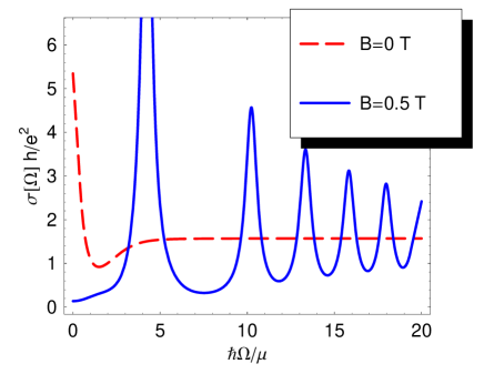
Figure 1: (Color online) The optical conductivity $\sigma_{xx}(\Omega)$ measured in $e^{2}/h$ units as a function of the frequency $\hbar\Omega/\mu$ for two different values of $B$ for $\mu=50\mbox{K}$, $T=15\mbox{K}$ and $\Gamma=10\mbox{K}$. We use $eB\to(4.5\times 10^{4}\mbox{K}^{2})B(\mbox{T})$.

Influence of the Landau quantization on the optical conductivity. We postpone a more comprehensive study of the influence of the gap $\Delta$ and the form of the function $\Gamma(\omega)$ on the ac conductivity for the future publication. Here to illustrate the behavior of $\sigma_{xx}(\Omega)$ described by Eq. (16) in Fig. 1 we show the results only for $\Delta=0$ and $\Gamma(\omega)=\mbox{const}$. One can see that for $B=0$ there is Drude peak. However, when the magnetic field is applied the spectral weight is transferred from the Drude peak to the resonance peaks in the agreement with a recent experiment Li2005 .

III.1 dc limits of the longitudinal and Hall conductivities

Let us firstly consider the dc limit of $\sigma_{xx}(\Omega)$,

$$\sigma_{xx}(\mu,B,T)=\sigma_{xx}(\Omega\to 0)=e^{2}N_{f}\int\limits_{-\infty}^{\infty}d\omega[-n_{F}^{\prime}(\omega)]\mathcal{A}_{L}(\omega,B,\Gamma,\Delta),$$ (19)

where

$$\begin{split}&\mathcal{A}_{L}(\omega,B,\Gamma,\Delta)=\frac{1}{\pi^{2}}\frac{\Gamma^{2}}{(v_{F}^{2}eB/c)^{2}+(2\omega\Gamma)^{2}}\\ &\times\left\{2\omega^{2}+\frac{(\omega^{2}+\Delta^{2}+\Gamma^{2})(v_{F}^{2}eB/c)^{2}-2\omega^{2}(\omega^{2}-\Delta^{2}+\Gamma^{2})v_{F}^{2}|eB|/c}{(\omega^{2}-\Delta^{2}-\Gamma^{2})^{2}+4\omega^{2}\Gamma^{2}}\right.\\ &\left.-\frac{\omega(\omega^{2}-\Delta^{2}+\Gamma^{2})}{\Gamma}\mbox{Im}\psi\left(\frac{\Delta^{2}-(\omega+i\Gamma)^{2}}{2v_{F}^{2}|eB|/c}\right)\right\},\end{split}$$ (20)

and $-n_{F}^{\prime}(\omega)=(1/4T)\cosh^{-2}[(\omega-\mu)/2T]$ is the derivative of the Fermi distribution. Here the scattering rate $\Gamma(\omega)$ remains a frequency dependent quantity. The expression (19) was originally derived in Refs. Gorbar2002PRB ; Sharapov2003PRB (see also Ferrer2003EPJB for a related derivation of the thermal conductivity) under the assumption $\Gamma(\omega)=\mbox{const}$.

Similarly to the dc expression (19) for $\sigma_{xx}$ one can take the dc limit $\Omega\to 0$ in Eq. (17) and obtain

$$\begin{split}\sigma_{xy}(\mu,B,T)=&\frac{e^{2}N_{f}{\rm sgn}(eB)}{2\pi^{2}}\int\limits_{-\infty}^{\infty}d\omega\left\{\left(-n_{F}(\omega)\right)^{\prime}\frac{B(\Gamma^{2}-\Delta^{2}+\omega^{2})}{B^{2}+4\omega^{2}\Gamma^{2}}\left[\frac{2\omega\Gamma(B+\Gamma^{2}+\Delta^{2}-\omega^{2})}{[\Gamma^{2}+(\Delta-\omega)^{2}][\Gamma^{2}+(\Delta+\omega)^{2}]}\right.\right.\\ &+\left.\left.{\rm Im}\psi\left(\frac{\Delta^{2}-(\omega+i\Gamma)^{2}}{2B}\right)\right]+n_{F}(\omega){\rm Im}\left[(1+i\Gamma^{\prime})\left(\frac{2(\omega+i\Gamma)}{B}+\frac{2(\omega+i\Gamma)}{\Delta^{2}-(\omega+i\Gamma)^{2}}\right.\right.\right.\\ &-\left.\left.\left.\frac{(\omega+i\Gamma)(\Delta^{2}-(\omega+i\Gamma)^{2})}{{B^{2}}}\psi^{\prime}\left(\frac{\Delta^{2}-(\omega+i\Gamma)^{2}}{2B}\right)\right)\right]\right\},\end{split}$$ (21)

where now $\Gamma^{\prime}\equiv d\Gamma(\omega)/d\omega$. The term with $n_{F}(\omega)$ can be integrated by parts and we finally arrive at

$$\sigma_{xy}=e^{2}N_{f}{\rm sgn}(eB)\int\limits_{-\infty}^{\infty}d\omega[-n_{F}^{\prime}(\omega)]\mathcal{A}_{H}(\omega,B,\Gamma,\Delta),$$ (22)

where

$$\begin{split}&\mathcal{A}_{H}(\omega,B,\Gamma,\Delta)=\frac{1}{2\pi^{2}}\left\{\frac{B(\Gamma^{2}-\Delta^{2}+\omega^{2})}{B^{2}+4\omega^{2}\Gamma^{2}}\frac{2\omega\Gamma(B+\Gamma^{2}+\Delta^{2}-\omega^{2})}{[\Gamma^{2}+(\Delta-\omega)^{2}][\Gamma^{2}+(\Delta+\omega)^{2}]}+\frac{2\omega\Gamma}{B}+\arctan\frac{\Delta+\omega}{\Gamma}-\arctan\frac{\Delta-\omega}{\Gamma}\right.\\ &-\left.2{\rm Im}\ln\Gamma\left(\frac{\Delta^{2}-(\omega+i\Gamma)^{2}}{2B}\right)+{\rm Im}\left[\left(\frac{B(\Gamma^{2}-\Delta^{2}+\omega^{2})}{B^{2}+4\omega^{2}\Gamma^{2}}+\frac{\Delta^{2}-(\omega+i\Gamma)^{2}}{B}\right)\psi\left(\frac{\Delta^{2}-(\omega+i\Gamma)^{2}}{2B}\right)\right]\right\}.\end{split}$$ (23)

Recall that here $B\equiv v_{F}^{2}|eB|/c$. Since we are considering non-interacting quasiparticles, the temperature and $\mu$ dependences of the conductivities (19) and (22) are only contained in the derivative of the Fermi distribution. The spectral function (23) for the Hall conductivity turns out to be more complicated than the corresponding function (20) for $\sigma_{xx}$, therefore it is useful to consider simple limiting cases and to establish the correspondence between our answer and the results obtained by previous authors.

IV Hall conductivity

IV.1 Classical limit $|eB|v_{F}^{2}/c\ll\Gamma^{2},\mu^{2}$. Drude-Zener formula

We begin our consideration with the classical limit $B\to 0$ (or more exactly $|eB|v_{F}^{2}/c\ll\Gamma^{2},\mu^{2}$), when Landau quantization is not essential. Using the asymptotic expansions

$$\begin{split}\ln\Gamma(z)&=\left(z-\frac{1}{2}\right)\ln z-z+\frac{1}{2}\ln(2\,\pi)+\frac{1}{12\,z}-\frac{1}{360\,z^{3}}+{O}\left(\frac{1}{z}\right)^{4},\\ \psi(z)&=\ln z-\frac{1}{2\,z}-\frac{1}{12\,z^{2}}+\frac{1}{120\,z^{4}}+O\left(\frac{1}{z^{5}}\right),\end{split}$$ (24)

we obtain that for $\Delta=0$ and $B\to 0$

$$\mathcal{A}_{H}(\omega,B,\Gamma,0)=\frac{1}{2\pi^{2}}\frac{B\Gamma}{1+B^{2}/(4\omega^{2}\Gamma^{2})}\frac{(3\Gamma^{4}-8\Gamma^{2}\omega^{2}-3\omega^{4})\Gamma\omega-3(\Gamma^{2}+\omega^{2})^{3}\arctan\frac{\omega}{\Gamma}}{6\Gamma^{3}\omega^{2}(\Gamma^{2}+\omega^{2})^{2}}.$$ (25)

Accordingly for the $T=0$ conductivity we find

$$\sigma_{xy}(\mu,B,0)=-\frac{e^{2}v_{F}^{2}N_{f}eB\mu^{2}\,\mbox{sgn}\mu}{2\pi c}\frac{1}{(v_{F}^{2}eB/c)^{2}+4\mu^{2}\Gamma^{2}},\qquad\Gamma\ll|\mu|,$$ (26)

where we restored $ev_{F}^{2}/c$. The diagonal conductivity (19) in the same limit reads

$$\sigma_{xx}=\frac{\sigma_{0}}{1+(\omega_{c}\tau)^{2}},\qquad\sigma_{0}=\frac{e^{2}N_{f}|\mu|}{4\pi\Gamma},$$ (27)

where the mean-free time of quasiparticles $\tau=1/2\Gamma$ enters instead of the transport time, $\tau_{tr}$ because we ignored the vertex corrections, and we introduced the cyclotron frequency,

$$\omega_{c}=\frac{|eB|v_{F}^{2}}{c|\mu|}=\frac{|eB|}{cm_{c}},\qquad m_{c}=\frac{|\mu|}{v_{F}^{2}}.$$ (28)

Here in the second equality $\omega_{c}$ is written in terms of an fictitious ”relativistic” mass, $m_{c}$ which plays the role of the cyclotron mass in the Lifshits-Kosevich formula Geim-new . The definition of $m_{c}$ shows that the chemical potential $|\mu|$ in graphene acquires also the meaning of the cyclotron mass, so that the latter is easily tunable by the gate voltage Geim-new .

Accordingly the Hall conductivity (26) can also be written in the Drude-Zener form

$$\sigma_{xy}=-\frac{\omega_{c}\tau\sigma_{0}\,\mbox{sgn}(eB)\,\mbox{sgn}\mu}{1+(\omega_{c}\tau)^{2}},$$ (29)

This result agrees with Eq. (23) of Ref. Zheng2002PRB when we take $\tau_{tr}=\tau=1/2\Gamma$ and $N_{f}=1$. As we will see later for $N_{f}=2$ all our results are twice bigger than the corresponding results of Refs. Zheng2002PRB ; Shon1998JPSJ .

Finally we consider the relationship (see Appendix C)

$$\rho=\frac{N_{f}}{2\pi\hbar^{2}v_{F}^{2}}\mu^{2}{\rm sgn\mu}$$ (30)

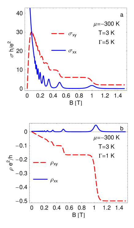
Figure 3: (Color online) (a) The Hall conductivity $\sigma_{xy}$ and the diagonal conductivity $\sigma_{xx}$ measured in $e^{2}/h$ units as a function of field $B$ for $\Gamma=5\mbox{K}$ for $\mu=-300\mbox{K}$ and $T=3\mbox{K}$. (b) The Hall resistivity $\rho_{xy}=-\sigma_{xy}/(\sigma_{xx}^{2}+\sigma_{xy}^{2})$ and the diagonal resistivity $\rho_{xx}=\sigma_{xx}/(\sigma_{xx}^{2}+\sigma_{xy}^{2})$ measured in $h/e^{2}$ units as a function of field $B$ for $\Gamma=1\mbox{K}$ for $\mu=-300\mbox{K}$ and $T=3\mbox{K}$. We use $eB\to(4.5\times 10^{4}\mbox{K}^{2})B(\mbox{T})$ and assume that $\Delta=0$.

between the chemical potential $\mu$ and carrier imbalance (density) $\rho$ for the relativistic quasiparticles [$\hbar$ is restored]. This relationship is in agreement with Fig. 3 d of Ref. Geim-new and with Ref. Kim-new , viz. the cyclotron mass in graphene, $m_{c}=(\pi\hbar^{2}|\rho|/v_{F}^{2})^{1/2}$ is indeed $\sim\sqrt{|\rho|}$. Since experiment Geim-new shows also that $\sigma_{0}\sim|\rho|$ for $B=0$, one may conclude that the carrier concentration dependence $\Gamma(\mu)\sim|\mu|^{-1}$ for $\Gamma\ll|\mu|$.

For the Hall resistivity one obtains from Eqs. (27) and (29) that

$$\rho_{xy}=-\frac{\sigma_{xy}}{\sigma_{xx}^{2}+\sigma_{xy}^{2}}=\frac{B}{ec\rho}.$$ (31)

Thus for weak magnetic field we arrive at the standard expression for the Hall coefficient $R_{H}=1/ec\rho$ which does not depend on the scattering mechanism and is used for measuring the carrier density.

IV.2 The limit $T\ll|\mu|\ll\sqrt{|eB|v_{F}^{2}/c},\Gamma$

Another interesting and analytically treatable limit is $T\ll|\mu|\ll\sqrt{|eB|},\Gamma$. Since for $T\to 0$ the derivative $-n_{F}^{\prime}(\omega)\to\delta(\omega-\mu)$, the Hall conductivity $\sigma_{xy}$ is directly expressed via Eq. (23) and we need only

$$\mathcal{A}_{H}(\mu,B,\Gamma,0)\simeq\frac{\mu B\Gamma}{2\pi^{2}}\left(\frac{4(B+\Gamma^{2})}{B^{2}\Gamma^{2}}-\frac{2\Gamma^{2}}{B^{3}}\psi^{\prime}\left(\frac{\Gamma^{2}}{2B}\right)\right),\qquad|\mu|\ll\sqrt{B},\Gamma.$$ (32)

Substituting in Eq. (32) the asymptotic expansion of $\psi^{\prime}(z)$ obtained from Eq. (24) in the limit $\sqrt{|eB|}\ll\Gamma$ we have

$$\mathcal{A}_{H}(\mu,B,\Gamma,0)\simeq-\frac{4\mu B}{3\pi^{2}\Gamma^{3}}.$$ (33)

Finally restoring the $ev_{F}^{2}/c$ factor, we obtain

$$\sigma_{xy}=-\frac{4e^{2}v_{F}^{2}N_{f}eB\mu}{3\pi^{2}c\Gamma^{3}},\qquad|\mu|\ll\sqrt{|eB|v_{F}^{2}/c}\ll\Gamma.$$ (34)

In the same limit the conductivity $\sigma_{xx}$ is “universal” Shon1998JPSJ ; Gorbar2002PRB ; foot3

$$\sigma_{xx}=\frac{e^{2}N_{f}}{\pi^{2}}.$$ (35)

Moreover, theoretically the universal value $(e^{2}/2\pi\hbar)(4/\pi)$ (or $e^{2}/\pi h$ per each type of carriers) is expected even in arbitrary fields Gorbar2002PRB , because the $n=0$ Landau level is field independent. (We note that $N_{f}=2$ when Zeeman splitting is neglected and $N_{f}=1$ when it is taken into account). The experiments Geim-new , however, show a bigger value of the conductivity per carrier type, $e^{2}/h$. Note also that in Ref. Suzuura2002 it is argued that for the long-range impurities in graphene the weak-localization correction makes a positive contribution to the conductivity $\sigma_{xx}$ that might explain the mentioned difference.

In the opposite limit, $\sqrt{|eB|}\gg\Gamma$ we find from Eq. (32) that ${\cal A}_{H}\simeq-2\mu/(\pi^{2}\Gamma)$ and, accordingly,

$$\sigma_{xy}=-\frac{2N_{f}e^{2}\mu}{\pi^{2}\Gamma},\qquad|\mu|\ll\Gamma\ll\sqrt{|eB|v_{F}^{2}/c}.$$ (36)

This limit is important in the strong field (Hall) regime at small carrier densities. It allows one to extract the impurities scattering rate $\Gamma$ studying the dependence of the Hall conductivity as a function of the chemical potential (or carrier density) in the vicinity of the point where the gate voltage changes its sign.

IV.3 Unusual quantization of the Hall conductivity in graphene

In this section we discuss a full derivation of Eqs. (4) – (6) from Ref. Gusynin2005PRL . Analyzing Eq. (6) of Ref. Gusynin2005PRL we demonstrated that the quantized Hall conductivity in graphene is equal to odd multiples of $2e^{2}/h$. Here we recapitulate the arguments of Ref. Gusynin2005PRL discussing a few interesting moments not mentioned there.

There are two ways to derive $\sigma_{xy}$ in the clean limit. The first option is to take the limit $\Gamma\to 0$ directly in Eq. (15) as was done in Ref. Gorbar2002PRB and the second option is to use a general expression (22). This option is considered in Appendix B, where we show that

$$\sigma_{xy}=-\frac{e^{2}N_{f}{\rm sgn}(eB)}{4\pi}\left[\tanh\frac{\mu+\Delta}{2T}+\tanh\frac{\mu-\Delta}{2T}+2\sum\limits_{n=1}^{\infty}\left(\tanh\frac{\mu+M_{n}}{2T}+\tanh\frac{\mu-M_{n}}{2T}\right)\right].$$ (37)

Note that $\sigma_{xy}$ is an antisymmetric function of $\mu$. Rearranging terms in Eq. (37) and using that $\tanh(\omega-\mu)/2T=1-2n_{F}(\omega)$ one can rewrite Eq. (37) in terms of the Fermi distribution

$$\sigma_{xy}=-\frac{e^{2}N_{f}{\rm sgn}(eB)}{2\pi}\sum\limits_{n=0}^{\infty}(2n+1)\left[n_{F}(M_{n})+n_{F}(-M_{n})-n_{F}(M_{n+1})-n_{F}(-M_{n+1})\right].$$ (38)

This representation for $\sigma_{xy}$ is an equivalent of Eq. (18) from Ref. Jonson1984PRB derived for an ideal two-dimensional electron gas

$$\sigma_{xy}=-\frac{e^{2}}{2\pi}\sum_{n=0}^{\infty}(n+1)[n_{F}(\omega_{n}^{\mathrm{nonrel}})-n_{F}(\omega_{n+1}^{\mathrm{nonrel}})],\qquad\omega_{n}^{\mathrm{nonrel}}=\frac{eB}{mc}\left(n+\frac{1}{2}\right),$$ (39)

where $m$ is the effective mass of the carriers with a parabolic dispersion law. The difference between the positions of Landau levels and their degeneracy for the Dirac quasiparticles and for nonrelativistic electron gas is encoded in the energies $M_{n}\sim\sqrt{n}$ and $\omega_{n}^{\mathrm{nonrel}}\sim(n+1/2)$ with $n=0,1,2,\ldots$, and in the different factors $2n+1$ and $n+1$ in Eqs. (38) and (39), respectively.

Now we rewrite Eq. (37) as follows Gorbar2002PRB

$$\sigma_{xy}=-\frac{e^{2}N_{f}\mbox{sgn}(eB)\mbox{sgn}\mu}{2\pi\hbar}\nu_{B},$$ (40)

with the filling factor foot1

$$\mbox{sgn}\mu\,\nu_{B}=\frac{1}{2}\left[\tanh\frac{\mu+\Delta}{2T}+\tanh\frac{\mu-\Delta}{2T}+2\sum\limits_{n=1}^{\infty}\left(\tanh\frac{\mu+M_{n}}{2T}+\tanh\frac{\mu-M_{n}}{2T}\right)\right].$$ (41)

Since we are considering the quantized Hall conductivity we restore Planck constant $h=2\pi\hbar$ in Eq. (40) and in what follows. Taking for definiteness $\mu>0$, $\Delta=0$ and using that $\tanh(\omega/2T)={\rm sgn}(\omega)$ for $T\to 0$, we obtain from Eq. (40) that

$$\sigma_{xy}=-\frac{e^{2}N_{f}\mbox{sgn}(eB)}{2\pi\hbar}\left[1+2\sum_{n=1}^{\infty}\theta(\mu-M_{n})\right]=-\frac{e^{2}N_{f}\mbox{sgn}(eB)}{h}\left(1+2\left[\frac{\mu^{2}c}{2\hbar|eB|v_{F}^{2}}\right]\right),$$ (42)

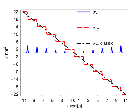
Figure 2: (Color online) The Hall conductivity $\sigma_{xy}$ and the diagonal conductivity $\sigma_{xx}$ measured in $e^{2}/h$ units as a function of the filling $\nu_{B}$ for $T=2\mbox{K}$, $\Gamma=1\mbox{K}$ and $B=2\mbox{T}$. We use $eB\to(4.5\times 10^{4}\mbox{K}^{2})B(\mbox{T})$ and assume that $\Delta=0$. The straight line corresponds to a classical dependence $\sigma_{xy}=-ec|\rho|\mbox{sgn}\mu/B$ [see Eq. (85)].

where $[x]$ denotes the integer part of $x$. The usual semi-phenomenological argumentation (see e.g. Ref. Hajdu.book ) for the occurrence of the IQHE states that in the presence of disorder when the dependence $\mu(\rho)$ becomes a smooth function, while the function $\sigma_{xy}(\mu)$ remains step-like. Accordingly, when in Eq. (42) the spin degeneracy is counted by choosing $N_{f}=2$, we arrive at the Hall quantization rule (1). The classical (85) and quantum (42) Hall conductivities coincide only for the odd fillings, $\nu_{B}=2n+1$ as shown in Fig. 2), where for comparison the dependence of $\sigma_{xx}(\nu_{B})$ is also plotted. As expected the minima of $\sigma_{xx}$ also occur at $\nu_{B}=2n+1$, while the peaks of $\sigma_{xx}$ coincide with the steps of $\sigma_{xy}(\nu_{B})$.

The appearance of the odd integer number in Eq. (1) rather than simply integer fillings is caused by the fact that the degeneracy of the $n=0$ Landau level is only half of the degeneracy of the levels with $n>0$ (see Appendix D). The lowest Landau level in the irreducible representation of the $2+1$ dimensional Dirac theory is special, because depending on which of two inequivalent irreducible representations is used it is occupied either by the electrons (fermions) or holes (antifermions) while at $n\geq 1$ there are solutions of the Dirac equation describing both electrons and holes (see Eq. (89)). The Dirac Lagrangian (2) which embeds a pair of independent $\mathbf{K}$ points on graphene’s Fermi surface, is written using a parity preserving $4\times 4$ reducible representation of $\gamma$ matrices that contains two irreducible representations with different parities. Therefore, the Landau levels associated with these $\mathbf{K}$ points merge into the full spectrum of the Dirac fermions in graphene. The superposition of the two spectra corresponding to the two inequivalent irreducible representations clearly explains a halved degeneracy of the lowest Landau level in graphene, because this level can be occupied by the holes from the $\mathbf{K}$ point (when $\mu<0$) and electrons from the $\mathbf{K}^{\prime}$ point (when $\mu>0$). This property of the $n=0$ level does not depend on whether the gap $\Delta$ has a finite value or $\Delta=0$. On the other hand, the higher levels may contain either electrons (when $\mu>0$) or holes (when $\mu<0$) both from $\mathbf{K}$ and $\mathbf{K}^{\prime}$ points.

The other way to explain the origin of “strange” odd numbers is to refer to, the mentioned above, positions of the minima of Shubnikov de Haas oscillations of $\sigma_{xx}$. Their unusual positions are caused by the phase shift of $\pi$ between the quantum magnetic oscillations for the relativistic quasiparticles (see Refs. Sharapov2004PRB ; Gusynin2005PRB ; Luk'yanchuk2004PRL ) and the corresponding oscillations for the nonrelativistic quasiparticles. The origin of the phase shift can be traced back to the different quantization of the relativistic, $M_{n}\sim\sqrt{n}$ and nonrelativistic $\omega_{n}^{\mathrm{nonrel}}\sim(n+1/2)$ Landau levels Sharapov2004PRB .

One can gain a deeper insight into this by considering the operator $\mathbb{S}=(1/2)\int d^{2}r[\Psi^{\dagger}(t,\mathbf{r}),S_{z}\Psi(t,\mathbf{r})]$, where $[,]$ is the commutator and the matrix

$$S_{z}=I_{2}\otimes(\sigma_{3}/2)=\left(\begin{array}[]{cc}\sigma_{3}/2&0\\ 0&\sigma_{3}/2\\ \end{array}\right).$$ (43)

The operator $\mathbb{S}$ generates the rotations of spinors in the plane by an angle $\phi$ that are described by the operator $U(\phi)=\exp(i\phi\mathbb{S})$. It is natural to interpret $\mathbb{S}$ as the pseudospin operator, because we use the spinors that are related to the presence of two sublattices in graphene. Each $\mathbf{K}$ point of graphene’s Fermi surface is characterized by a two-component spinor and there are two inequivalent $\mathbf{K}$ points. There is a temptation to make a direct analogy between the pseudospin operator $\mathbb{S}$ and the spin operator in $3+1$ dimensional Dirac theory. This, however, is misleading because the very notion of the spin in $2+1$ and $3+1$ dimensions is meaningful only for a massive particle. For a massless particle in $3+1$ dimension instead of spin one introduces the helicity which characterizes the projection of its spin on the direction of momentum. Since in $2+1$ dimensional case one cannot make rotations around the direction of the quasiparticle momentum lying in the two-dimensional plane, the helicity concept for massless particles is meaningless in this case. Indeed, one can check that the pseudospin operator $\mathbb{S}$ is identically zero for free massless Dirac particles.

Nevertheless, below we argue that for the massless quasiparticles in graphene in an external magnetic field the pseudospin acquires a new meaning closely related to the Berry’s phase discussed in the different context Luk'yanchuk2004PRL ; Kim-new .

One can obtain (see Appendix D) for $eB>0$ and $N_{f}=1$ that

$$\mathbb{S}=\frac{1}{2}\left[\sum_{m=-\infty}^{0}\left(b_{0m}^{\dagger}b_{0m}-c_{0m}^{\dagger}c_{0m}\right)+\sum_{n=1}^{\infty}\sum_{m=-\infty}^{n}\frac{\Delta}{M_{n}}\left(a_{nm}^{\dagger}a_{nm}+b_{nm}^{\dagger}b_{nm}-c_{nm}^{\dagger}c_{nm}-d_{nm}^{\dagger}d_{nm}\right)\right],$$ (44)

where $a_{nm}$ ($b_{nm}$) are the annihilation operators of fermions with energies $M_{n}$ given by Eq. (6) (antifermions with energies $-M_{n}$) for $\mathbf{K}$ point and $c_{nm}$ ($d_{nm}$) are annihilation operators of fermions (antifermions) for $\mathbf{K}^{\prime}$ point. The quantum number $m\leq n$ in Eq. (44) reflects the degeneracy of each level in angular momentum. Interestingly in the limit $\Delta\to 0$ only the $n=0$ level contributes to $\mathbb{S}$, so that the notion of the pseudospin is meaningful only for the states from the lowest Landau level, i.e. for the zero modes.

Let us now consider the rotation by the angle $\phi=2\pi$ of a quasiparticle state $|n=0\rangle=b_{0m}^{\dagger}|0\rangle$ from the $n=0$ level. Here $|0\rangle$ is the vacuum state. For $\Delta=0$ one can show that $U(2\pi)|n=0\rangle=\exp(i\pi)|n=0\rangle$, i.e. after the rotation by $2\pi$ the quasiparticle state from the lowest Landau level changes its phase by $\pi$. On the other hand, the states from the levels with $n\geq 1$ remain invariant, because for $\Delta=0$ the operator $U(\phi)$ does not contain the operators that can change these states. It occurs exactly due to this Berry’s phase shift for massless quasiparticles from the $n=0$ level in the external field, that the carriers in graphene cannot be considered as simply very light carriers with a finite mass. Note that in $3+1$ dimensional Dirac theory all fermionic states acquire the phase shift by $\pi$ after the rotation by $\phi=2\pi$.

If the $n=0$ level had the same degeneracy as the higher levels, the Hall conductivity would had been quantized in a more conventional manner,

$$\sigma_{xy}^{\mathrm{semicond}}=-\frac{4e^{2}}{h}n,\qquad n=0,1,\ldots$$ (45)

which one might expect for a two-band [the first band would corresponds to the electrons with $\omega_{n}=M_{n}-\mu$ and the second band, accordingly, to the holes with $\omega_{n}=-M_{n}-\mu$], two-valley [corresponding to $\mathbf{K}$ and $\mathbf{K}^{\prime}$ points of graphen’s Fermi surface] semiconductor. Again in Eq. (45) we assumed that $e,B,\mu>0$

It is appropriate here to mention that although the conventional quantized Hall conductance $\sigma_{xy}=-(e^{2}/h)n$ with $n=0,1,\ldots$ is often derived by solving the nonrelativistic Schrödinger equation, it was shown MacDonald1983PRB ; Nieto1985AJP that there are no relativistic corrections to this expression and the same result remains valid for a relativistic electron gas confined in the plane described by the $(3+1)$ dimensional Dirac equation. The case of graphene is different, because the Dirac theory is used to describe an effective theory of non-relativistic quasiparticles with a linear dispersion. Although one usually associates the Dirac-like description of graphene with a linear dispersion of quasiparticle excitations, $E(\mathbf{k})=-\mu\pm v_{F}|\mathbf{k}|$ for $B=0$, the quantization (1) survives even when there is a nonzero gap $\Delta$.

Another important feature of graphene is that its Dirac-like description is based on the $4\times 4$ reducible, parity preserving representation of $\gamma$ matrices which allows one to include two inequivalent $\mathbf{K}$ points of graphene’s Fermi surface. From a theoretical point of view one may also choose a separate $\mathbf{K}$ point and consider the role of the parity breaking terms (see e.g. Refs. Haldane1988PRL ; Schakel1991PRD ). This approach is closely related to early unsuccessful Abouelsaood1985PRL attempts to explain the IQHE using the chiral anomaly. However, in the case of the parity anomaly the Hall effect occurs even in zero magnetic field and in the absence of Landau levels Haldane1988PRL . On the contrary, the Dirac-like description of graphene preserves parity, so that the Hall conductivity is always absent in zero magnetic field.

IV.4 Illustrations of analytical results for the Hall conductivity

Fig. 2 is plotted to illustrate the odd integer Hall quantization (1) and it is computed on the base of Eqs. (22) and (23). Since the representation (22), (23) is derived under the approximations discussed in Secs. II and III, this consideration ignores the presence of localized states. Thus for finite scattering rate $\Gamma$ this representation for $\sigma_{xy}(B,\Gamma,\Delta)$ provides only an approximate description of the Hall quantization, because $\Gamma$ remains nonzero even between Landau levels. Nevertheless, considering the relative simplicity and analytical character of the two expressions (19) for $\sigma_{xx}$ and (22) for $\sigma_{xy}$, overall they give an amazingly good description of the conductivities. In particular, one can see $\sigma_{xx}$ is indeed very small in the plateaux regions of $\sigma_{xy}$.

The IQHE can be obtained by varying either carrier concentration as done in Fig. 2 or the value of the applied magnetic field. The latter possibility is shown in Fig. 3, where both conductivities (Fig. 3 a) and resistivities (Fig. 3 b) are plotted at $T=3\mbox{K}$. To observe the quantum Hall effect in conventional semiconductors one should go down to the temperatures lower than $10\mbox{K}$, while in graphene it can be observed up to $100\mbox{K}$. This wider range of temperatures is related to the fact that for the Dirac quasiparticles the distance between Landau levels is much larger than for the nonrelativistic quasiparticles in the same applied field, so that some signatures of Shubnikov de Haas oscillations remain notable even at room temperature Geim-new .

Although the definition of the filling factor foot1 does not depend on whether relativistic or nonrelativistic quasiparticles are considered, the relationship (30) between the chemical potential and carrier imbalance shows that the small filling factors become accessible in relatively small, compared to conventional semiconductors, fields. These features make the IQHE in graphene very promising for fundamental research and possible applications.

Finally one can observe that $\sigma_{xy}=0$ for $B\to 0$. This illustrates the point mentioned in Sec. IV.3 that the IQHE in graphene is conventional in the sense that its explanation does not rely on any kind of parity breaking anomaly Haldane1988PRL ; Schakel1991PRD .

IV.5 Magnetic catalysis and its observation in the Hall conductivity

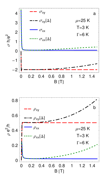
Figure 4: (Color online) The Hall conductivity $\sigma_{xy}$ and the diagonal conductivity $\sigma_{xx}$ measured in $e^{2}/h$ units as a function of field $B$ for $\Gamma=6\mbox{K}$ for $\mu=25\mbox{K}$ and $T=3\mbox{K}$. The dash-dotted (black) and dotted (green) lines are calculated using $\Delta(B)$ given by Eq. (46). (b) The Hall resistivity $\rho_{xy}$ and the diagonal resistivity $\rho_{xx}$ measured in $h/e^{2}$ units as a function of field $B$ for $\Gamma=6\mbox{K}$ for $\mu=25\mbox{K}$ and $T=3\mbox{K}$. The dash-dotted (black) and dotted (green) lines are calculated using $\Delta(B)$ given by Eq. (46). We use $eB\to(4.5\times 10^{4}\mbox{K}^{2})B(\mbox{T})$.

The flat, field independent behavior of $\sigma_{xx}(B)$ and $\sigma_{xy}(B)$ for $B\gtrsim 1.1\mbox{T}$ seen in Fig. 3 corresponds to the regime where only the lowest Landau level is filled, because it always stays below the chemical potential (except for $\mu=0$). As we already mentioned in Sec. II, it was predicted in Refs. Gusynin1995PRD ; Gorbar2002PRB that for Dirac fermions in $2+1$ there is a phenomenon called magnetic catalysis. It is expected that above a critical field $B_{c}$ which is a function of $\mu$ and $T$, a gap $\Delta$ should open in the spectrum of the Dirac fermions. Since the conditions for the magnetic catalysis are the most favorable at low carrier concentrations (or $\mu\approx 0$), in Fig. 4 we present the behavior of $\sigma_{xy}(B,\Delta(B))$ and $\sigma_{xx}(B,\Delta(B))$ for $|\mu|$ smaller than was used to plot Fig. 3. For comparison we plot these conductivities both for $\Delta=0$ and for the phenomenological gap dependence

$$\Delta(B)=c\sqrt{B-B_{c}}\theta(B-B_{c}),$$ (46)

where $c$ is some constant. As stated above, $B_{c}=B_{c}(\mu,T)$, but for illustrative purposes we simply choose an arbitrary value $B_{c}=0.3\mbox{T}$. As one can clearly see, the opening of the gap $\Delta$ causes the decrease of $|\sigma_{xy}(B)|$ from the last plateau value $2e^{2}/h$. This tendency can also be understood from Eq. (37). In the strong field limit the sum over $M_{n}$ with $n>0$ does not contribute and we obtain (for $eB>0$ and $\mu>0$)

$$\sigma_{xy}=-\frac{e^{2}N_{f}}{4\pi\hbar}\left[\tanh\frac{\mu+\Delta(B)}{2T}+\tanh\frac{\mu-\Delta(B)}{2T}\right]\to-\frac{e^{2}N_{f}}{2\pi\hbar}\theta(\mu-\Delta(B)),\qquad T\to 0.$$ (47)

Eq. (47) shows that when $\Delta(B)>\mu$ the magnetic catalysis leads to a formation of a new insulating phase. On the other hand, we observe in Fig. 4 (a) that $\sigma_{xx}(B)$ increases as the gap opens, while the increase of the diagonal resistivity (Fig. 4 (b)) also indicates the system goes towards an insulating phase.

In our consideration we assumed that the opening of the gap $\Delta$ does not affect the chemical potential $\mu$. We will come back to this important issue in Sec. V.2.

V Hall angle and Nernst coefficient

The approach presented allows one to calculate other transport coefficients such as thermal conductivity $\kappa_{ij}(B,\Gamma,\Delta)$ [see Refs. Ferrer2003EPJB ; Sharapov2003PRB ; Gusynin2005PRB , where the diagonal thermal conductivity is studied] and Peltier (thermoelectric) conductivity $\beta_{ij}(B,\Gamma,\Delta)$ tensors. The calculation of the off-diagonal coefficients involves some subtleties, because the conventional Kubo expressions have to be altered Smrcka1997JPC ; Oji1985PRB ; Cooper1997PRB to reflect the role of magnetization on the electronic thermal transport in applied field. However in the low-temperature limit one may rely on the Sommerfeld expansion and express the thermoelectric tensor through the conductivity tensor

$$\beta_{ij}=-\frac{\pi^{2}}{3}\frac{T}{e}\frac{\partial\sigma_{ij}}{\partial\mu}.$$ (48)

The Nernst signal measured in the absence of electric current is expressed in terms of $\sigma_{ij}$ and $\beta_{ij}$ as

$$e_{y}(T,B)\equiv-\frac{E_{y}}{\nabla_{x}T}=\frac{\sigma_{xx}\beta_{xy}-\sigma_{xy}\beta_{xx}}{\sigma_{xx}^{2}+\sigma_{xy}^{2}}.$$ (49)

Since in the low-temperature limit Eq. (48) is valid, the Nernst signal (49) can be found differentiating the Hall angle

$$\Theta_{H}=\arctan\frac{\sigma_{xy}}{\sigma_{xx}}$$ (50)

via the relation

$$e_{y}(T,B)=-\frac{\pi^{2}}{3}\frac{T}{e}\frac{\partial\Theta_{H}}{\partial\mu}.$$ (51)

Here based on the results derived in the previous sections, we will study the behavior of the Hall angle and Nernst coefficient.

V.1 Drude-Zener $|eB|v_{F}^{2}/c\ll\Gamma^{2}\ll\mu^{2}$ and $T\ll|\mu|\ll\sqrt{|eB|v_{F}^{2}/c}\ll\Gamma$ limits

In the classical limit (see Sec. IV.1) $\sigma_{xy}$ and $\sigma_{xx}$ are given by Eqs. (29) and (27), respectively. Hence,

$$\Theta_{H}\simeq\tan\Theta_{H}=-\omega_{c}\tau\,\mbox{sgn}(eB)\,\mbox{sgn}\mu=-\frac{v_{F}^{2}eB}{2c\Gamma\mu}.$$ (52)

The Hall angle (29) diverges at $\mu\to 0$, but one should consider only finite values of $\mu$, because it is derived under the assumption $|eB|v_{F}^{2}/c\ll\Gamma^{2}\ll\mu^{2}$. Accordingly when $\mu$ is small, Eq. (29) is valid only for very low fields $B$. When the character of the carriers changes from hole-like ($\mu<0$) to electron-like ($\mu>0$), the Hall angle also changes from positive to negative. The behavior of the Nernst signal

$$e_{y}=-\frac{\pi^{2}}{3}\frac{k_{B}^{2}Tv_{F}^{2}B}{2c\Gamma\mu^{2}}$$ (53)

mirrors the divergence of the Hall angle at $\mu\to 0$, but $e_{y}<0$ irrespective of the sign of $\mu$. [Boltzmann constant $k_{B}$ is restored in Eq. (53).] Eqs. (52) and (53) agree with the results obtained in Ref. Oganesyan2004PRB using Boltzmann theory. This is not surprising, because this is exactly the limit described by Drude-Zener theory. We note that although in Ref. Oganesyan2004PRB the so called $d$-density-wave state is considered, a direct comparison with our case is possible, because the effective low-energy Dirac theory turns out to be the same Sharapov2003PRB .

Since in the regime $T\ll|\mu|\ll\sqrt{|eB|v_{F}^{2}/c}\ll\Gamma$ the conductivities $\sigma_{xx}$ and $\sigma_{xy}$ are given by Eqs. (35) and (34), respectively, for the Hall angle one obtains

$$\Theta_{H}=-\frac{4v_{F}^{2}eB\mu}{3c\Gamma^{3}}.$$ (54)

Hence the Nernst signal is positive and given by

$$e_{y}\simeq\frac{4\pi^{2}}{9}\frac{k_{B}^{2}Tv_{F}^{2}B}{c\Gamma^{3}}.$$ (55)

The Nernst signal (55) can be very large in clean system because $e_{y}\sim\tau^{3}$ Oganesyan2004PRB . This regime is accessible due to the fact that $\mu\approx 0$, i.e. one may consider the large and positive Nernst signal as another fingerprint of the Dirac quasiparticles. We mention that since the Dirac quasiparticles emerge in the scenarios with unconventional charge density waves (UCDW) Nersesyan1989JLTP ; Dora2003PRB , in Ref. Dora2003PRB the large and positive $e_{y}$ is regarded as a hallmark of UCDW.

V.2 Illustrations of analytical results and detection of the gap $\Delta$ from the Hall angle measurements

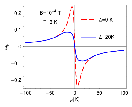
Figure 5: (Color online) The Hall angle $\Theta_{H}$ as a function of chemical potential $\mu$ for two different values of $\Delta$ for $B=10^{-4}\mbox{T}$, $T=3\mbox{K}$ and $\Gamma=1\mbox{K}$. We use $eB\to(4.5\times 10^{4}\mbox{K}^{2})B(\mbox{T})$.

In Fig. 5 and 6 we present the dependence of the Hall angle (50) on $\mu$ for two different values of the field $B$. The case of small $B$ shown in Fig. 5 agrees with the analytical expressions discussed above. Indeed when $|\mu|$ decreases, there is an increase of $\Theta_{H}$ [cf. Eq.(52)] followed by the regime where $\Theta_{H}$ crosses zero [cf. Eq. (54)].

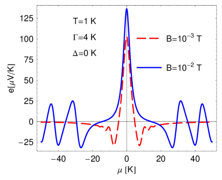
Figure 7: (Color online) The Nernst signal $e_{y}$ in $\mu V/K$ as a function of chemical potential $\mu$ for two different values of $B$ for $T=1\mbox{K}$, $\Gamma=4\mbox{K}$ and $\Delta=0\mbox{K}$. We use $eB\to(4.5\times 10^{4}\mbox{K}^{2})B(\mbox{T})$.

In Fig. 7 and 8 we show the behavior of the Nernst signal. When $|\mu|$ is large and $B$ is small, $e_{y}<0$ and rather small. However, when $|\mu|$ decreases, $e_{y}$ becomes positive and large ($\sim 100\mu V/K$) in accord with Eq. (55). When the field $B$ increases, the value $e_{y}(\mu=0)$ becomes even larger and for finite $\mu$ there are oscillations of $e_{y}(\mu)$.

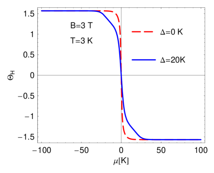
Figure 6: (Color online) The Hall angle $\Theta_{H}$ as a function of chemical potential $\mu$ for two different values of $\Delta$ for $B=3\mbox{T}$, $T=3\mbox{K}$ and $\Gamma=1\mbox{K}$. We use $eB\to(4.5\times 10^{4}\mbox{K}^{2})B(\mbox{T})$.

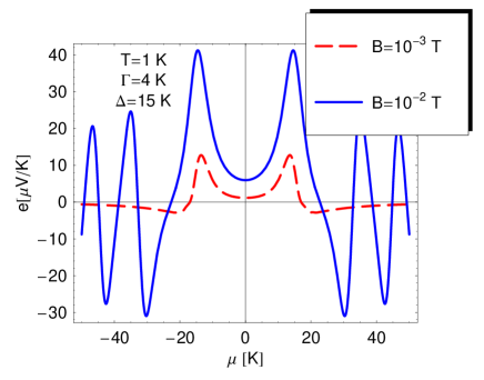
Figure 8: (Color online) The Nernst signal $e_{y}$ in $\mu V/K$ as a function of chemical potential $\mu$ for two different values of $B$ for $T=1\mbox{K}$, $\Gamma=4\mbox{K}$ and $\Delta=15\mbox{K}$. We use $eB\to(4.5\times 10^{4}\mbox{K}^{2})B(\mbox{T})$.

Analyzing Figs. 5 – 8 one may discover another interesting property, viz. in the presence of a nonzero gap $\Delta$ the dependence $\Theta_{H}(\mu,\Delta)$ in Figs. 5, 6 near $\mu\approx 0$ is not so steep as compared to the $\Delta=0$ case. Accordingly this feature is reflected in the Nernst signal, so that a finite $\Delta$ also shows up in the dependence $e_{y}(\mu,\Delta)$ as a dip. Thus we suggest that careful study of the Hall angle $\Theta_{H}(\mu,\Delta)$ and Nernst signal $e_{y}(\mu,\Delta)$ may help to establish the presence of a nonzero gap $\Delta$ in graphene.

It is important, however, to stress that the gap is detectable only if its opening does not change the chemical potential $\mu$. The situation is exactly the same as in Ref. Sharapov2003PRB , where we considered the possibility of detecting the gap using precise measurements of the period of the quantum magnetic oscillations (de Haas van Alphen or Shubnikov de Haas). In the clean system with a fixed carrier density $\rho$, the chemical potential $\mu$ is given by the number equation (84). The opening of the gap $\Delta$ results in the adjustment of $\mu$, so that the gap cannot be detected neither from the period of the oscillations Sharapov2003PRB nor from the Hall angle. Nevertheless, the observation of the quantum Hall effect Geim-new ; Kim-new shows that there is localization and the chemical potential remains fixed making the gap detection possible.

Finally we stress that here we neglected the dependence of $\Gamma(\mu)$, while a simple argument given at the end of Sec. IV.1 shows that this carrier concentration dependence is rather important.

VI Conclusions

In this paper we have studied the dc Hall conductivity, Hall angle and Nernst signal in a planar system with relativistic Dirac-like spectrum of quasiparticle excitations. We also presented the results for the diagonal optical conductivity in the external magnetic field perpendicular to the plane.

Our main results can be summarized as follows.
(1) We have obtained analytical expressions for the diagonal optical conductivity $\sigma_{xx}(\Omega,\mu,B,T,\Delta)$ [Eq. (16)] and the off-diagonal optical conductivity $\sigma_{xy}(\Omega,\mu,B,T,\Delta)$ [Eq. (17)].

(2) We have derived the analytical expression (22) with the kernel (23) for the dc Hall conductivity $\sigma_{xy}(\mu,B,T,\Delta)$ which includes an arbitrary impurity scattering rate $\Gamma(\omega)$ that was assumed to be independent of the Landau level index $n$.

(3) We have shown that in the classical limit our expression for dc Hall conductivity Eq. (22) reduces to the conventional Drude-Zener formula (29).

(4) The direct comparison of the expression (39) derived in Ref. Jonson1984PRB for Hall conductivity in a two-dimensional electron gas with the corresponding representation (38) for graphene allows one to understand the origin of the odd integer Hall quantization Eq. (1) in graphene in terms of the difference between the energies and degeneracies of the Landau levels in these systems.

(5) In Sec. IV.3 we presented the arguments (using the second quantization formalism) that the nontrivial Berry’s phase in graphene is associated with the anomalous properties of the zero modes or the quasiparticles from the lowest Landau level.

(6) We have investigated the behavior of the Hall angle and the Nernst signal showing that for $\mu\approx 0$ there is an interesting regime [see Eq. (55)] where the Nernst signal is strong and positive.

(7) On the basis of the results obtained, we have discussed in Secs. IV.5 and V.2 the possibility of detecting a gap $\Delta$ that may open in the spectrum of the Dirac-like quasiparticle excitations of graphene due to a nontrivial interaction between them.

All our results are derived for noninteracting quasiparticles treating the impurity scattering rate $\Gamma(\omega)$ as a phenomenological parameter and without considering the interaction with impurities that would demand solving an equation for $\Gamma(\omega,\mu)$ (see Ref. Zheng2002PRB ). Accordingly we did not consider the problems related to localization and a full explanation of the IQHE (see Refs. Hajdu.book ; Prange-book ). These problems by themselves acquire a new depth and deserve a separate study. For example, it is pointed out in Ref. Geim-new that localization effects in graphene are suppressed. Interestingly, it is shown in Ref. Suzuura2002 that for long-range impurities the weak-localization correction makes a positive contribution to the conductivity $\sigma_{xx}$. This anti-localization property is related in Ref. Suzuura2002 to the Berry’s phase of the Dirac fermions. Definitely, such effects were not considered in the present work. Nevertheless we hope that the approach presented here allows one to explain in the most transparent way the difference between the Dirac quasiparticles in graphene and nonrelativistic quasiparticles in conventional semiconductors when these systems are placed in a magnetic field.

VII Acknowledgments

We thank P. Esquinazi, A. Geim, W.A. de Heer, P. Kim and Y. Kopelevich for discussing with us their experimental results and J.P. Carbotte, E.V. Gorbar, V.M. Loktev, V.A. Miransky and E.A. Pashitsky for illuminating discussions. The work of V.P.G. was supported by the SCOPES-project IB7320-110848 of the Swiss NSF. S.G.Sh. was supported by the Natural Science and Engineering Research Council of Canada (NSERC) and by the Canadian Institute for Advanced Research (CIAR).

Appendix A Calculation of $\sigma_{ij}(\Omega)$

The most efficient way of calculating $\sigma_{ij}(\Omega)$ is to use again the spectral representation Eq. (13) (for $\mu=0$). This allows one to eliminate one of the integrations over frequency in Eq. (15), so that for the real part of the conductivity (9) we obtain

$$\begin{split}\sigma_{ij}(\Omega)&=\frac{e^{2}v_{F}^{2}}{2\pi\Omega}\,{\rm Re}\int\limits_{-\infty}^{\infty}d\omega\,\int\frac{d^{2}k}{(2\pi)^{2}}{\rm tr}\left\{[n_{F}(\omega)-n_{F}(\omega+\Omega)]\gamma^{i}S^{R}(\omega+\Omega,\mathbf{k})\gamma^{j}S^{A}(\omega,\mathbf{k})\right.\\ &-\left.n_{F}(\omega)\gamma^{i}S^{R}(\omega+\Omega,\mathbf{k})\gamma^{j}S^{R}(\omega,\mathbf{k})+n_{F}(\omega+\Omega)\gamma^{i}S^{A}(\omega+\Omega,\mathbf{k})\gamma^{j}S^{A}(\omega,\mathbf{k})\right\}.\end{split}$$ (56)

Using the expressions Eq. (8) for the advanced and retarded Green’s functions we obtain

$$\begin{split}&\sigma_{ij}(\Omega)=\frac{e^{2}v_{F}^{2}}{2\pi\Omega}\,\,{\rm Re}\int\limits_{-\infty}^{\infty}d\omega\int\frac{d^{2}k}{(2\pi)^{2}}e^{-\frac{c{\mathbf{k}}^{2}}{|eB|}}\sum\limits_{n,m=0}^{\infty}(-1)^{n+m}{\rm tr}\Biggl{\{}[n_{F}(\omega)-n_{F}(\omega+\Omega)]\\ &\times\left.\frac{\gamma^{i}S^{R}_{n}(\omega+\Omega)\gamma^{j}S^{A}_{m}(\omega)}{[(\omega+\Omega+i\Gamma(\omega+\Omega))^{2}-M_{n}^{2}][(\omega-i\Gamma(\omega))^{2}-M_{m}^{2}]}-n_{F}(\omega)\frac{\gamma^{i}S^{R}_{n}(\omega+\Omega)\gamma^{j}S^{R}_{m}(\omega)}{[(\omega+\Omega+i\Gamma(\omega+\Omega))^{2}-M_{n}^{2}][(\omega+i\Gamma(\omega))^{2}-M_{m}^{2}]}\right.\\ &+n_{F}(\omega+\Omega)\frac{\gamma^{i}S^{A}_{n}(\omega+\Omega)\gamma^{j}S^{A}_{m}(\omega)}{[(\omega+\Omega-i\Gamma(\omega+\Omega))^{2}-M_{n}^{2}][(\omega-i\Gamma(\omega))^{2}-M_{m}^{2}]}\Biggr{\}},\end{split}$$ (57)

where $S_{n}^{(R,A)}$ are the numerators of Eq. (8) obtained from Eq. (7) for $S_{n}(i\omega_{n},\mathbf{k})$ via the rule $S_{n}^{(R,A)}(\omega,\mathbf{k})=S_{n}(i\omega_{n}\to\omega\pm i\Gamma(\omega))$. This allows to include the frequency dependent impurity scattering rate, $\Gamma(\omega)$. The traces in Eq. (57) are easily evaluated

$$\begin{split}&{\rm tr}\left[\gamma^{i}S_{n}^{(R,A)}(\omega^{\prime})\gamma^{j}S_{m}^{(R,A)}(\omega)\right]=-8N_{f}[(\omega^{\prime}\pm i\Gamma^{\prime})(\omega\pm i\Gamma)-\Delta^{2}]\left[\delta_{ij}\left(L_{n}(x)L_{m-1}(x)+L_{n-1}(x)L_{m}(x)\right)\right.\\ &\left.+i\epsilon_{ij}\,{\rm sgn}(eB)\left(L_{n}(x)L_{m-1}(x)-L_{n-1}(x)L_{m}(x)\right)\right]-64N_{f}(2k_{i}k_{j}-\delta_{ij}\mathbf{k}^{2})L_{n-1}^{1}(x)L_{m-1}^{1}(x),\end{split}$$ (58)

where $\epsilon_{ij}$ is antisymmetric tensor ($\epsilon_{12}=1$) and the argument of the Laguerre polynomials is $x=2c{\bf{k}}^{2}/|eB|$. Integrating over momenta we obtain

$$\begin{split}\sigma_{ij}(\Omega)&=\frac{e^{2}v_{F}^{2}|eB|N_{f}}{2\pi^{2}c\,\Omega}\,\,{\rm Re}\sum\limits_{n,m=0}^{\infty}(-1)^{n+m+1}\left[\delta_{ij}(\delta_{n,m-1}+\delta_{n-1,m})+i\epsilon_{ij}\,{\rm sgn}(eB)(\delta_{n,m-1}-\delta_{n-1,m})\right]\\ &\times\int\limits_{-\infty}^{\infty}d\omega\left[\frac{[n_{F}(\omega)-n_{F}(\omega^{\prime})][(\omega^{\prime}+i\Gamma^{\prime})(\omega-i\Gamma)-\Delta^{2}]}{[(\omega^{\prime}+i\Gamma^{\prime})^{2}-M_{n}^{2}][(\omega-i\Gamma)^{2}-M_{m}^{2}]}-\frac{n_{F}(\omega)[(\omega^{\prime}+i\Gamma^{\prime})(\omega+i\Gamma)-\Delta^{2}]}{[(\omega^{\prime}+i\Gamma^{\prime})^{2}-M_{n}^{2}][(\omega+i\Gamma)^{2}-M_{m}^{2}]}\right.\\ &+\left.\frac{n_{F}(\omega^{\prime})[(\omega^{\prime}-i\Gamma^{\prime})(\omega-i\Gamma)-\Delta^{2}]}{[(\omega^{\prime}-i\Gamma^{\prime})^{2}-M_{n}^{2}][(\omega-i\Gamma)^{2}-M_{m}^{2}]}\right].\end{split}$$ (59)

The Kronnecker’s delta symbols appeared in Eq. (59) are due to the the orthogonality relation for the Laguerre polynomials,

$$\int_{0}^{\infty}dxe^{-x}x^{\alpha}L_{m}^{\alpha}(x)L_{n}^{\alpha}(x)=\frac{\Gamma(n+\alpha+1)}{n!}\delta_{mn},$$ (60)

show that only transitions between neighboring Landau levels contribute in the conductivity. The last term of Eq. (LABEL:trace-S_n) vanished after the angular integration. The real part of Eq. (59) reads

$$\begin{split}\sigma_{ij}(\Omega)&=\frac{e^{2}v_{F}^{2}|eB|N_{f}}{2\pi^{2}c\,\Omega}\sum\limits_{n,m=0}^{\infty}(-1)^{n+m+1}\int\limits_{-\infty}^{\infty}d\omega\left\{\delta_{ij}(\delta_{n,m-1}+\delta_{n-1,m})[n_{F}(\omega)-n_{F}(\omega^{\prime})]{\rm Re}[\Pi^{1}_{n,m}(\omega,\omega^{\prime})-\Pi^{2}_{n,m}(\omega,\omega^{\prime})]\right.\\ &-\left.\epsilon_{ij}\,{\rm sgn}(eB)(\delta_{n,m-1}-\delta_{n-1,m})[[n_{F}(\omega)-n_{F}(\omega^{\prime})]{\rm Im}\Pi^{1}_{n,m}(\omega,\omega^{\prime})-[n_{F}(\omega)+n_{F}(\omega^{\prime})]{\rm Im}\Pi^{2}_{n,m}(\omega,\omega^{\prime})]\right\},\end{split}$$ (61)

where we introduced

$$\Pi^{1}_{n,m}(\omega,\omega^{\prime})=\frac{(\omega^{\prime}+i\Gamma^{\prime})(\omega-i\Gamma)-\Delta^{2}}{[(\omega^{\prime}+i\Gamma^{\prime})^{2}-M_{n}^{2}][(\omega-i\Gamma)^{2}-M_{m}^{2}]},\quad\Pi^{2}_{n,m}(\omega,\omega^{\prime})=\frac{(\omega^{\prime}+i\Gamma^{\prime})(\omega+i\Gamma)-\Delta^{2}}{[(\omega^{\prime}+i\Gamma^{\prime})^{2}-M_{n}^{2}][(\omega+i\Gamma)^{2}-M_{m}^{2}]}.$$ (62)

When we derived Eq. (61) we used the fact that the real part of $\Pi^{1,2}_{n,m}$ does not alter when the simultaneous replacements $i\Gamma\to-i\Gamma$ and $i\Gamma^{\prime}\to-i\Gamma^{\prime}$ are made, while its imaginary part reverses sign. These features of $\sigma_{ij}(\Omega)$ are also used below when Eqs. (16) and (17) are written in the symmetric form. The sum over $m$ in Eq. (61) is easily calculated using Kronnecker delta’s,

$$\begin{split}\sigma_{ij}(\Omega)&=\frac{e^{2}v_{F}^{2}|eB|N_{f}}{2\pi^{2}c\,\Omega}\sum\limits_{n=0}^{\infty}\int\limits_{-\infty}^{\infty}d\omega\left\{\delta_{ij}[n_{F}(\omega)-n_{F}(\omega^{\prime})]{\rm Re}[\Pi^{1}_{n,n+1}(\omega,\omega^{\prime})+\Pi^{1}_{n+1,n}(\omega,\omega^{\prime})-\Pi^{2}_{n,n+1}(\omega,\omega^{\prime})\right.\\ &-\left.\Pi^{2}_{n+1,n}(\omega,\omega^{\prime})]-\epsilon_{ij}\,{\rm sgn}(eB)\left[[n_{F}(\omega)-n_{F}(\omega^{\prime})]{\rm Im}[\Pi^{1}_{n,n+1}(\omega,\omega^{\prime})-\Pi^{1}_{n+1,n}(\omega,\omega^{\prime})]\right.\right.\\ &-\left.\left.[n_{F}(\omega)+n_{F}(\omega^{\prime})]{\rm Im}[\Pi^{2}_{n,n+1}(\omega,\omega^{\prime})-\Pi^{2}_{n+1,n}(\omega,\omega^{\prime})]\right]\right\}.\end{split}$$ (63)

Further summation over $n$ can be performed expanding $\Pi^{1,2}$ in terms of the partial fractions,

$$\begin{split}\Pi^{1}_{n,m}(\omega,\omega^{\prime})&=\frac{(\omega^{\prime}+i\Gamma^{\prime})(\omega-i\Gamma)-\Delta^{2}}{[\omega-\omega^{\prime}-i(\Gamma+\Gamma^{\prime})][\omega+\omega^{\prime}-i(\Gamma-\Gamma^{\prime})]+2B(n-m)}\left[\frac{1}{(\omega^{\prime}+i\Gamma^{\prime})^{2}-M_{n}^{2}}-\frac{1}{(\omega-i\Gamma)^{2}-M_{m}^{2}}\right],\\ \Pi^{2}_{n,m}(\omega,\omega^{\prime})&=\frac{(\omega^{\prime}+i\Gamma^{\prime})(\omega+i\Gamma)-\Delta^{2}}{[\omega-\omega^{\prime}+i({\Gamma-\Gamma^{\prime}})][\omega+\omega^{\prime}+i({\Gamma+\Gamma^{\prime}})]+2B(n-m)}\left[\frac{1}{(\omega^{\prime}+i\Gamma^{\prime})^{2}-M_{n}^{2}}-\frac{1}{(\omega+i\Gamma)^{2}-M_{m}^{2}}\right],\end{split}$$ (64)

where for brevity we introduced the notation $B\equiv v_{F}^{2}|eB|/c$. The resulting sums are expressed via the digamma function by means of the formula

$$\sum\limits_{n=0}^{\infty}\left[\frac{A}{n+a}+\frac{B}{n+b}+\frac{C}{n+c}+\frac{D}{n+d}\right]=-[A\psi(a)+B\psi(b)+C\psi(c)+D\psi(d)],$$ (65)

where for convergence $A+B+C+D=0$, so that we arrive at the final expressions for the conductivities (16) and (17). In the limit of vanishing magnetic field the Hall conductivity becomes zero, while for the longitudinal conductivity we obtain

$$\begin{split}\sigma_{xx}(\Omega)&=\frac{e^{2}N_{f}}{2\pi^{2}\Omega}{\rm Re}\int\limits_{-\infty}^{\infty}d\omega[n_{F}(\omega)-n_{F}(\omega+\Omega)]\left[\left(\frac{(\omega+i\Gamma)(\omega^{\prime}+i\Gamma^{\prime})-\Delta^{2}}{[\omega-\omega^{\prime}+i(\Gamma-\Gamma^{\prime})][\omega+\omega^{\prime}+i(\Gamma+\Gamma^{\prime})]}\right.\right.\\ &-\left.\left.\frac{(\omega+i\Gamma)(\omega^{\prime}-i\Gamma^{\prime})-\Delta^{2}}{[\omega-\omega^{\prime}+i(\Gamma+\Gamma^{\prime})][\omega+\omega^{\prime}+i(\Gamma-\Gamma^{\prime})]}\right)\ln[{\Delta^{2}-(\omega+i\Gamma)^{2}}]+(\omega\leftrightarrow\omega^{\prime},\Gamma\leftrightarrow\Gamma^{\prime})\right].\end{split}$$ (66)

Calculating the real part we can represent the last expression in the form

$$\sigma_{xx}(\Omega)=\frac{e^{2}N_{f}}{2\pi^{2}}\int\limits_{-\infty}^{\infty}d\omega\left[\frac{n_{F}(\omega)-n_{F}(\omega+\Omega)}{\Omega}\right]{{\cal A}_{L}(\omega,\Omega,\Gamma,\Delta)},$$ (67)

where

$$\begin{split}{\cal A}_{L}(\omega,\Omega,\Gamma,\Delta)=\frac{1}{D(\omega,\omega^{\prime})}&\left[a\ln\frac{(\Delta^{2}+\Gamma^{\prime 2}-\omega^{\prime 2})^{2}+4\omega^{\prime 2}\Gamma^{\prime 2}}{(\Delta^{2}+\Gamma^{2}-\omega^{2})^{2}+4\omega^{2}\Gamma^{2}}\right.\\ &\left.+b\arctan\frac{2\omega\Gamma}{\Delta^{2}+\Gamma^{2}-\omega^{2}}+c\arctan\frac{2\omega^{\prime}\Gamma^{\prime}}{\Delta^{2}+\Gamma^{\prime 2}-\omega^{\prime 2}}\right],\end{split}$$ (68)

and

$$\begin{split}D&(\omega,\omega^{\prime})=[(\Gamma-\Gamma^{\prime})^{2}+(\omega-\omega^{\prime})^{2}][(\Gamma+\Gamma^{\prime})^{2}+(\omega-\omega^{\prime})^{2}][(\Gamma-\Gamma^{\prime})^{2}+(\omega+\omega^{\prime})^{2}][(\Gamma+\Gamma^{\prime})^{2}+(\omega+\omega^{\prime})^{2}],\\ a=&{\Gamma\Gamma^{\prime}}\left[(\omega^{\prime 2}-\omega^{2}+\Gamma^{\prime 2}-\Gamma^{2})[(\omega^{\prime 2}+\omega^{2}+\Gamma^{\prime 2}+\Gamma^{2})^{2}+4(\omega^{\prime 2}\omega^{2}-\Gamma^{\prime 2}\Gamma^{2})]-8\Delta^{2}\omega\omega^{\prime}(\omega^{\prime 2}-\omega^{2}-\Gamma^{\prime 2}+\Gamma^{2})\right],\\ b=&2\left[\omega\Gamma^{\prime}(\omega^{\prime 2}+\omega^{2}+\Gamma^{\prime 2}+\Gamma^{2})[(\omega^{\prime 2}-\omega^{2})^{2}+(\Gamma^{\prime 2}-\Gamma^{2})^{2}+2(\omega^{\prime 2}+\omega^{2})(\Gamma^{\prime 2}+\Gamma^{2})-8\omega^{\prime 2}\Gamma^{2}]\right.\\ &\left.-2\Delta^{2}\omega^{\prime}\Gamma^{\prime}[(\omega^{\prime 2}-\omega^{2})^{2}+(\Gamma^{\prime 2}-\Gamma^{2})^{2}+2(\omega^{\prime 2}+\omega^{2})(\Gamma^{\prime 2}+\Gamma^{2})-8\omega^{2}\Gamma^{2}]\right],\\ c=&2\left[\omega^{\prime}\Gamma(\omega^{\prime 2}+\omega^{2}+\Gamma^{\prime 2}+\Gamma^{2})[(\omega^{\prime 2}-\omega^{2})^{2}+(\Gamma^{\prime 2}-\Gamma^{2})^{2}+2(\omega^{\prime 2}+\omega^{2})(\Gamma^{\prime 2}+\Gamma^{2})-8\omega^{2}\Gamma^{\prime 2}]\right.\\ &\left.-2\Delta^{2}\omega\Gamma[(\omega^{\prime 2}-\omega^{2})^{2}+(\Gamma^{\prime 2}-\Gamma^{2})^{2}+2(\omega^{\prime 2}+\omega^{2})(\Gamma^{\prime 2}+\Gamma^{2})-8\omega^{\prime 2}\Gamma^{\prime 2}]\right].\end{split}$$ (69)

For $\Delta=0$ these expressions are simplified:

$$\begin{split}&a={\Gamma\Gamma^{\prime}}(\omega^{\prime 2}-\omega^{2}+\Gamma^{\prime 2}-\Gamma^{2})[(\omega^{\prime 2}+\omega^{2}+\Gamma^{\prime 2}+\Gamma^{2})^{2}+4(\omega^{\prime 2}\omega^{2}-\Gamma^{\prime 2}\Gamma^{2})],\\ &b=2\left[\omega\Gamma^{\prime}(\omega^{\prime 2}+\omega^{2}+\Gamma^{\prime 2}+\Gamma^{2})[(\omega^{\prime 2}-\omega^{2})^{2}+(\Gamma^{\prime 2}-\Gamma^{2})^{2}+2(\omega^{\prime 2}+\omega^{2})(\Gamma^{\prime 2}+\Gamma^{2})-8\omega^{\prime 2}\Gamma^{2}]\right],\\ &c=2\left[\omega^{\prime}\Gamma(\omega^{\prime 2}+\omega^{2}+\Gamma^{\prime 2}+\Gamma^{2})[(\omega^{\prime 2}-\omega^{2})^{2}+(\Gamma^{\prime 2}-\Gamma^{2})^{2}+2(\omega^{\prime 2}+\omega^{2})(\Gamma^{\prime 2}+\Gamma^{2})-8\omega^{2}\Gamma^{\prime 2}]\right].\end{split}$$ (70)

The behavior of $\sigma_{xx}(\Omega)$ in this limit was studied in Ref. Ando2002JPSJ for graphene and in Ref. Kim2004PRB for a $d$-wave superconductor. For $B=0$ the latter is rather similar to graphene at $\mu=0$.

Appendix B Derivation of the Hall conductivity in the clean limit from Eq. (22)

Eq. (37) can be obtained directly from Eq. (22) . Indeed taking the limit $\Gamma\to 0$, we find from Eq. (23) that

$$\mathcal{A}_{H}(\omega,B,\Gamma,\Delta)=\frac{1}{2\pi^{2}}\left[\arctan\frac{2\omega\Gamma}{\Delta^{2}+\Gamma^{2}-\omega^{2}}-2{\rm Im}\ln\Gamma\left(\frac{\Delta^{2}+\Gamma^{2}-\omega^{2}-2i\omega\Gamma}{B}\right)\right],\quad\Gamma\to 0.$$ (71)

Recall that here $B$ is a short-hand notation for $v_{F}^{2}|eB|/c$. We begin with the expression

$$\begin{split}&{\rm Im}\ln\Gamma\left(\frac{\Delta^{2}+\Gamma^{2}-\omega^{2}-2i\omega\Gamma}{2B}\right)={\rm sgn}\,\omega{\rm Im}\ln\Gamma\left(\frac{\Delta^{2}+\Gamma^{2}-\omega^{2}-2i|\omega|\Gamma}{2B}\right)\\ &={\rm sgn}\,\omega{\rm Im}\ln\Gamma\left(\frac{\Delta^{2}+\Gamma^{2}-\omega^{2}-2i|\omega|\Gamma}{2B}\right)\left[\theta(\Delta^{2}+\Gamma^{2}-\omega^{2})+\theta(\omega^{2}-\Delta^{2}-\Gamma^{2})\right].\end{split}$$ (72)

Now we use the relationship

$$\Gamma(z)\Gamma(-z)=\frac{\pi}{z\sin(-\pi z)}$$ (73)

to rewrite the last expression in the form

$$\begin{split}&{\rm Im}\ln\Gamma\left(\frac{\Delta^{2}+\Gamma^{2}-\omega^{2}-2i\omega\Gamma}{2B}\right)=-{\rm sgn}\,\omega\left\{{\rm Im}\ln\Gamma\left(\frac{|\omega^{2}-\Delta^{2}-\Gamma^{2}|+2i|\omega|\Gamma}{2B}\right)\right.\\ &\left.+\theta(\omega^{2}-\Delta^{2}-\Gamma^{2})\left[\pi-\arctan\frac{2|\omega|\Gamma}{|\omega^{2}-\Delta^{2}-\Gamma^{2}|}+{\rm Im}\ln\sin\left(\pi\frac{\omega^{2}-\Delta^{2}-\Gamma^{2}+2i|\omega|\Gamma}{2B}\right)\right]\right\}.\end{split}$$ (74)

Hence

$$\begin{split}&\mathcal{A}_{H}(\omega,B,\Gamma,\Delta)=\frac{{\rm sgn}\,\omega}{2\pi^{2}}\left\{\arctan\frac{2|\omega|\Gamma}{|\omega^{2}-\Delta^{2}-\Gamma^{2}|}+2{\rm Im}\ln\Gamma\left(\frac{|\omega^{2}-\Delta^{2}-\Gamma^{2}|+2i|\omega|\Gamma}{2B}\right)\right.\\ &\left.-\theta(\omega^{2}-\Delta^{2}-\Gamma^{2})\left[\pi-2{\rm Im}\ln\sin\left(\pi\frac{\omega^{2}-\Delta^{2}-\Gamma^{2}+2i|\omega|\Gamma}{2B}\right)\right]\right\}.\end{split}$$ (75)

Now using the formula

$${\rm Im}\ln\sin(a+ib)=\frac{\pi}{2}-a-\sum\limits_{k=1}^{\infty}\frac{1}{k}\sin(2ka)e^{-2kb},\quad b>0,$$ (76)

we arrive at the following representation

$$\begin{split}&\mathcal{A}_{H}(\omega,B,\Gamma,\Delta)=\frac{{\rm sgn}\,\omega}{2\pi^{2}}\left\{\arctan\frac{2|\omega|\Gamma}{|\omega^{2}-\Delta^{2}-\Gamma^{2}|}+2{\rm Im}\ln\Gamma\left(\frac{|\omega^{2}-\Delta^{2}-\Gamma^{2}|+2i|\omega|\Gamma}{2B}\right)\right.\\ &\left.-\pi\theta(\omega^{2}-\Delta^{2}-\Gamma^{2})\left[\frac{\omega^{2}-\Delta^{2}-\Gamma^{2}}{B}+2\sum\limits_{k=1}^{\infty}\frac{1}{\pi k}\sin\left(2\pi k\frac{\omega^{2}-\Delta^{2}-\Gamma^{2}}{2B}\right)e^{-\frac{2k|\omega|\Gamma}{B}}\right]\right\}.\end{split}$$ (77)

Finally by means of the identity (4.6) of Ref. Sharapov2004PRB , we obtain in the limit $\Gamma\to 0$ that

$$\begin{split}&\mathcal{A}_{H}(\omega,B,\Gamma,\Delta)=-\frac{1}{2\pi}{\rm sgn}\,\omega\theta(\omega^{2}-\Delta^{2})\left[\frac{\omega^{2}-\Delta^{2}}{B}+2\sum\limits_{k=1}^{\infty}\frac{1}{\pi k}\sin\left(2\pi k\frac{\omega^{2}-\Delta^{2}}{2B}\right)\right]\\ &=-\frac{1}{2\pi}{\rm sgn}\,\omega\left[\theta(\omega^{2}-\Delta^{2})+2\sum\limits_{n=1}^{\infty}\theta(\omega^{2}-\Delta^{2}-2Bn)\right].\end{split}$$ (78)

Inserting the last expression in Eq. (22) and integrating over $\omega$ we finally arrive at Eq. (37).

Appendix C The equation for chemical potential

To derive the relationship for the carrier imbalance $\rho$ ($\rho\equiv n_{e}-n_{h}$, where $n_{e}$ and $n_{h}$ are the densities of “electrons” and “holes”, respectively) and the chemical potential $\mu$, we begin with the well-known expression

$$\rho=\mbox{tr}[\gamma^{0}\tilde{S}(\tau,\mathbf{0})],\quad\tau\to 0,$$ (79)

where $\tilde{S}(\tau,\mathbf{r})$ is the translation invariant part of the Green’s function (4). Taking its Fourier transform and using the spectral representation (13), we arrive at

$$\rho=T\sum\limits_{n=-\infty}^{\infty}\int\frac{d^{2}k}{(2\pi)^{2}}\int_{-\infty}^{\infty}d\omega\frac{{\rm tr}[\gamma^{0}A(\omega,{\bf k})]}{i\omega_{n}+\mu-\omega}.$$ (80)

After evaluating the sum over Matsubara frequencies we obtain

$$\rho=-\frac{1}{2}\int\frac{d^{2}k}{(2\pi)^{2}}\int_{-\infty}^{\infty}d\omega\tanh\frac{\omega-\mu}{2T}{\rm tr}[\gamma^{0}A(\omega,{\bf k})].$$ (81)

Now taking into account that ${\rm tr}[\gamma^{0}A(\omega,{\bf k})]$ is an even function of $\omega$, we may write

$$\begin{split}\rho=&\frac{1}{2}\int\frac{d^{2}k}{(2\pi)^{2}}\int_{0}^{\infty}d\omega\left[\tanh\frac{\omega+\mu}{2T}-\tanh\frac{\omega-\mu}{2T}\right]{\rm tr}[\gamma^{0}A(\omega,{\bf k})]\\ =&\int\frac{d^{2}k}{(2\pi)^{2}}\int_{0}^{\infty}d\omega\left[n_{F}(\omega-\mu)-n_{F}(\omega+\mu)\right]{\rm tr}[\gamma^{0}A(\omega,{\bf k})].\end{split}$$ (82)

Substituting the spectral function (14) in the first line of the last equation and integrating over momenta, we arrive at

$$\rho=\frac{N_{f}|eB|}{4\pi^{2}c}\sum\limits_{n=0}^{\infty}\alpha_{n}\int_{-\infty}^{\infty}d\omega\tanh\frac{\omega+\mu}{2T}\left(\frac{\Gamma}{(\omega-M_{n})^{2}+\Gamma^{2}}+(\omega\to-\omega)\right),\quad\alpha_{0}=1,\quad\alpha_{n}=2,\,n\geq 1.$$ (83)

The ratio $\alpha_{n}/\alpha_{0}=2$ for $n\geq 1$ is related to the above-mentioned smaller degeneracy of the $n=0$ Landau level. It is easy to see that Eq. (83) in the limit $\Gamma=0$ reduces to

$$\rho=\frac{N_{f}|eB|}{4\pi c}\left[\tanh\frac{\mu+\Delta}{2T}+\tanh\frac{\mu-\Delta}{2T}+2\sum\limits_{n=1}^{\infty}\left(\tanh\frac{\mu+M_{n}}{2T}+\tanh\frac{\mu-M_{n}}{2T}\right)\right],$$ (84)

while in the limit $B=\Gamma=T=\Delta=0$ it reduces to Eq. (30) (see, for example, Eq. (77) in Ref. Gorbar2002PRB ) giving the relationship between the chemical potential and the free carrier imbalance.

Comparing Eq. (84) with Eq. (37) we finally obtain that in the ideally clean system (see also Ref. Gorbar2002PRB )

$$\sigma_{xy}=-\frac{ec\rho}{B}.$$ (85)

The last expression seems to be paradoxical at first glance, because it corresponds to the classical expression (31) far beyond the validity of the classical limit (see Sec. IV.1). Nevertheless this result is absolutely correct and it shows the consistency of our calculation. As explained in Ref. Girvin-lectures , Eq. (85) is expected for an ideal conductor. This similarity between Eq. (84) and Eq. (37) was exploited in Ref. Schakel1991PRD , where instead of calculating the electrical conductivity $\sigma_{xy}$, the density (84) was obtained. However, to consider the IQHE one must take into account the presence of impurities Hajdu.book ; Girvin-lectures ; Prange-book . It is believed that they lead to the localization of most of the bulk states, except in a region around the center of the Landau band, and act as a reservoir which almost fixes the chemical potential Hajdu.book ; Prange-book . It turns out that in this more physical situation it still makes sense to rely on Eq. (37) for $\sigma_{xy}$, while Eq. (84) cannot be used in the IQHE regime. One particular model of the equation for $\mu$ that includes the reservoir could be a generalization of the one discussed in Ref. Grigoriev2001JETP for nonrelativistic quasiparticles.

The main implication of this model is that the density of the delocalized carriers in the Hall bar may oscillate as the field $B$ varies. It seems the oscillations of this kind were indeed observed in the IQHE system Raymond1999ApplSurf . However, there is no consensus on a microscopic picture of the localization in the quantum Hall effect (see e.g. Refs. Huckestein1995RMP ; Ilani2004Nature ; Steele2005PRL ) even in 2D electron gas. On the other hand, the localization of the Dirac quasiparticles appears to be quite different from the localization in 2D electron gas with the parabolic dispersion Geim-new . This indicates that further studies of the localization and oscillations of the density of the delocalized carriers in graphene may be very useful.

Appendix D Solution of the Dirac equation in the symmetric gauge

The Dirac equation in the problem of a relativistic fermion in a constant magnetic field $B$ takes the following form in $2+1$ dimensions:

$$\left[i\tilde{\gamma}^{0}\hbar\partial_{t}+iv_{F}\tilde{\gamma}^{1}\left(\hbar\partial_{x}+i\frac{e}{c}A_{x}^{\mathrm{ext}}\right)+iv_{F}\tilde{\gamma}^{2}\left(\hbar\partial_{y}+i\frac{e}{c}A_{y}^{\mathrm{ext}}\right)-\Delta\right]\psi(t,{\mathbf{r}})=0,$$ (86)

where the vector potential $\mathbf{A}^{ext}=(-By/2,Bx/2)$, so that the magnetic field $\mathbf{B}=\nabla\times\mathbf{A}^{\mathrm{ext}}$ is directed along the positive z axis. In $2+1$ dimensions, there are two inequivalent representations of the Dirac algebra (see e.g.,Ref. Jackiw1981PRD ):

$$\tilde{\gamma}^{0}=\sigma_{3},\tilde{\gamma}^{1}=i\sigma_{1},\tilde{\gamma}^{2}=i\sigma_{2}$$ (87)

and

$$\tilde{\gamma}^{0}=-\sigma_{3},\tilde{\gamma}^{1}=-i\sigma_{1},\tilde{\gamma}^{2}=-i\sigma_{2}.$$ (88)

which correspond to right- and left-handed coordinate systems. Here $\sigma_{i}$ are Pauli matrices. The representation of gamma matrices $(\sigma_{3},i\sigma_{2},-i\sigma_{1})$ used to write the Lagrangian (2) is related to the representation $(\sigma_{3},i\sigma_{1},i\sigma_{2})$ by means of the unitary transformation $U=(\hat{I}+i\sigma_{3})/\sqrt{2}$. Although the final results of the calculations do not depend on either the representation of $\gamma$-matrices or the gauge, the intermediate expressions depend on this choice.

Since the representation (87), (88) is more commonly used in the literature, in this Appendix we solve the Dirac equation (86) and obtain the operator (44) using this representation.

Let us begin by considering the representation (87). The energy spectrum in the problem (86) depends on the sign of $eB$; let us for definiteness assume that $eB>0$. Then, the energy spectrum takes the form (to be concrete, we assume also that $\Delta\geq 0$):

$$\begin{split}E_{0}&=-M_{0}=-\Delta,\\ E_{n}&=\pm M_{n}=\pm\sqrt{\Delta^{2}+2n{|eB|\hbar v_{F}^{2}}/{c}},\quad n=1,2,\dots\end{split}$$ (89)

(the Landau levels). The general solution is

$$\psi(x)=\sum_{n,m}\left[a_{nm}u_{nm}(x)+b^{+}_{nm}v_{nm}(x)\right],$$ (90)

where

$$\begin{split}&u_{nm}=\frac{1}{l\sqrt{2\pi}}\exp(-iM_{n}t)\frac{1}{\sqrt{2M_{n}}}\left(\begin{array}[]{cc}\sqrt{M_{n}+\Delta}\,J^{n-m}_{m-1}(\xi)e^{i(m-1)\theta}\\ \sqrt{M_{n}-\Delta}\,J^{n-m}_{m}(\xi)e^{im\theta}\end{array}\right),\quad n\geq 1,\quad m\leq n,\\ &v_{0m}=\frac{1}{l\sqrt{2\pi}}\exp(iM_{0}t)\left(\begin{array}[]{cc}0\\ J^{-m}_{m}(\xi)e^{im\theta}\end{array}\right),\quad n=0,\quad m\leq 0,\\ &v_{nm}=\frac{1}{l\sqrt{2\pi}}\exp(iM_{n}t)\frac{1}{\sqrt{2M_{n}}}\left(\begin{array}[]{cc}-\sqrt{M_{n}-\Delta}\,J^{n-m}_{m-1}(\xi)e^{i(m-1)\theta}\\ \sqrt{M_{n}+\Delta}\,J^{n-m}_{m}(\xi)e^{im\theta}\end{array}\right),\quad n\geq 1,\quad m\leq n.\end{split}$$ (91)

Here the functions Melrose

$$J^{n}_{\nu}(\xi)=\left[\frac{n!}{(n+\nu)!}\right]^{1/2}e^{-\xi/2}\xi^{\nu/2}L_{n}^{\nu}(\xi),\qquad J_{m}^{-m}(\xi)=\frac{(-1)^{m}}{\sqrt{(-m)!}}e^{-\xi/2}\xi^{-m/2}\quad(m\leq 0),$$ (92)

where $L_{n}^{m}(\xi)$ are Laguerre polynomials ($L_{n}^{m}(\xi)\equiv 0$ for $n\leq-1$), $l\equiv(\hbar c/|eB|)^{1/2}$ is the magnetic length, $\xi={\mathbf{r}}^{2}/2l^{2}$, the quantum number $m\leq n$ reflects the degeneracy of each level in the angular momentum. The spinors $u_{nm}$ and $v_{nm}$ are normalized as follows:

$$\int\,d^{2}x\,u_{n^{\prime}m^{\prime}}^{\dagger}(x)u_{nm}(x)=\int\,d^{2}x\,v_{n^{\prime}m^{\prime}}^{\dagger}(x)v_{nm}(x)=\delta_{n^{\prime},n}\delta_{m^{\prime},m}.$$ (93)

Thus the lowest Landau level with $n=0$ is special: while at $n\geq 1$, there are solutions corresponding to both fermion $(E_{n}=M_{n})$ and antifermion $(E_{n}=-M_{n})$ states, the solution with $n=0$ describes only antifermion states.

If we used the representation (88) for Dirac’s matrices, the general solution would be given by Eq. (90) with $u_{nm}(x)$, $v_{nm}(x)$ being substituted by $v_{nm}(-x),u_{nm}(-x)$:

$$\psi(x)=\sum\limits_{n,m}\left[c_{nm}v_{nm}(-x)+d_{nm}^{\dagger}u_{nm}(-x)\right].$$ (94)

The solution $v_{0m}$ corresponds to the Landau level $n=0$ with positive energy $E_{0}=\Delta$, while the solutions $v_{nm},u_{nm}$ with $n\geq 1$ correspond to the energy eigenvalues $E_{n}=\pm M_{n}$ (compare with Eq. (D4)). Accordingly, when the spectra for two inequivalent representations are united together the degeneracy of the $n=0$ level turns out to be a half of the degeneracy of the levels with $n\geq 1$. The four-component spinor $\Psi$ is composed from two two-component spinors Eqs. (90) and (94) and using it one can obtain the expression (44) for the pseudospin rotation generator.

References

- (1) K.S. Novoselov, A.K. Geim, S.V. Morozov, D. Jiang, Y. Zhang, S.V. Dubonos, I.V. Grigorieva, and A.A. Firsov, Science 306, 666 (2004); K.S. Novoselov, A.K. Geim, S.V. Morozov, S.V. Dubonos, Y. Zhang, and D. Jiang, cond-mat/0410631.
- (2) K.S. Novoselov, D. Jiang, T. Booth, V.V. Khotkevich, S.M. Morozov, A.K. Geim, Proc. Nat. Acad. Sc. 102, 10451 (2005); see also the latest work on bilayer graphene, K.S. Novoselov, E. McCann, S.V. Morozov, V.I. Fal’ko, M.I. Katsnelson, U. Zeitler, D. Jiang, F. Schedin and A. K. Geim, Nature Physics 22, 177 (2006).
- (3) C. Berger, Z. Song, T. Li, X. Li, A.Y. Ogbazghi, R. Feng, Z. Dai, A.N. Marchenkov, E.H. Conrad, P.N. First, and W.A. de Heer, J. Phys. Chem. B 108, 19912 (2004).
- (4) Y. Zhang, J.P. Small, M.E.S. Amori, and P. Kim, Phys. Rev. Lett. 94, 176803 (2005).
- (5) J.S. Bunch, Y. Yaish, M. Brink, K. Bolotin, and P.L. McEuen, Nano Letters 5, 287 (2005).
- (6) S.V. Morozov, K.S. Novoselov, F. Schedin, D. Jiang, A.A. Firsov, and A.K. Geim, Phys. Rev. B72, 201401(R) (2005).
- (7) K.S. Novoselov, A.K. Geim, S.V. Morozov, D. Jiang, M.I. Katsnelson, I.V. Grigorieva, S.V. Dubonos, A.A. Firsov, Nature 438, 197 (2005).
- (8) Y. Zhang, Y.-W. Tan, H.L. Stormer, P. Kim, Nature 438, 201 (2005).
- (9) G.W. Semenoff, Phys. Rev. Lett. 53, 2449 (1984).
- (10) J. Gonzàlez, F. Guinea, and M.A.H. Vozmediano, Nucl. Phys. B 406, 771 (1993).
- (11) V.P. Gusynin and S.G. Sharapov, Phys. Rev. Lett. 95, 146801 (2005).
- (12) N.M.R. Peres, F. Guinea, A.H. Castro Neto, preprint cond-mat/0506709.
- (13) G. Dresselhaus, Phys. Rev. B 10, 3602 (1974).
- (14) S. Uji, J.S. Brooks, and Y. Iye, Physica B 246-247, 299 (1998).
- (15) Y. Kopelevich, J.H.S. Torres, R.R. da Silva, F. Mrowka, H. Kempa, and P. Esquinazi, Phys. Rev. Lett. 90, 156402 (2003).
- (16) H. Kempa, P. Esquinazi, Y. Kopelevich, Solid State Commun. 138, 118 (2006).
- (17) R. Ocaña, P. Esquinazi, H. Kempa, J.H.S. Torres, and Y. Kopelevich, Phys. Rev. B68, 165408 (2003).
- (18) S.G. Sharapov, V.P. Gusynin, and H. Beck, Phys. Rev. B 69, 075104 (2004).
- (19) V.P. Gusynin and S.G. Sharapov, Phys. Rev. B 71, 125124 (2005).
- (20) I.A. Luk’yanchuk and Y. Kopelevich, Phys. Rev. Lett. 93, 166402 (2004).
- (21) T. Matsui, H. Kambara, Y. Niimi, K. Tagami, M. Tsukada, and H. Fukuyama Phys. Rev. Lett. 94, 226403 (2005).
- (22) Z. Li, W. Padilla, S. Dordevic, P. Esquinazi, C.C. Homes, D. Basov, Abstracts of March 2005 APS Meeting.
- (23) A.A. Nersesyan and G.E. Vachanadze, J. Low Temp. Phys. 77, 293 (1989); A.A. Nersesyan, G.I. Japaridze, and G.E. Vachanadze, J. Phys. Cond. Matt. 3, 3353 (1991).
- (24) E. Beaugnon and R. Tournier, Nature 349, 470 (1991).
- (25) E.V. Gorbar, V.P. Gusynin, V.A. Miransky, and I.A. Shovkovy, Phys. Rev. B 66, 045108 (2002).
- (26) S.G. Sharapov, V.P. Gusynin, and H. Beck, Phys. Rev. B 67, 144509 (2003).
- (27) Y. Zhang, Z. Jiang, J.P. Small, M.S. Purewal, Y.-W. Tan, M. Fazlollahi, J.D. Chudow, J.A. Jaszczak, H.L. Stormer, P. Kim, Phys. Rev. Lett. 96, 136806 (2006).
- (28) R. Saito, G. Dresselhaus and M.S. Dresselhaus, Physical Properties of Carbon Nanotubes (Imperial College Press, London, 1998).
- (29) D.V. Khveshchenko, Phys. Rev. Lett. 87, 246802 (2001); D.V. Khveshchenko and H. Leal, Nucl. Phys. B 687, 323 (2004).
- (30) V.P. Gusynin, V.A. Miransky, and I.A. Shovkovy, Phys. Rev. Lett. 73, 3499 (1994); Phys. Rev. D 52, 4718 (1995).
- (31) A. Chodos, K.Everding, and D.A. Owen, Phys. Rev. D 42, 2881 (1990).
- (32) Y. Zheng and T. Ando, Phys. Rev. B 65, 245420 (2002).
- (33) T. Champel and V.P. Mineev, Phys. Rev. B 66, 195111 (2002); 67, 089901(E) (2003).
- (34) E.J. Ferrer, V.P. Gusynin, and V. de la Incera, Eur. Phys. J. B 33, 397 (2003).
- (35) N.H. Shon and T. Ando, J.Phys. Soc. Jpn. 67, 2421 (1998).
- (36) This universality has the same origin as the universality considered in E. Fradkin, Phys. Rev. B 33, 3263 (1986) for degenerate semiconductors and in P.A. Lee, Phys. Rev. Lett. 71, 1887 (1993) for -wave superconductors in the absence of magnetic field.
- (37) H. Suzuura and T. Ando, Physics of Semiconductors 2002, edited by A. R. Long and J.H. Davies (Institute of Physics Publishing, Bristol, 2003).
- (38) M. Jonson and S. M. Girvin, Phys. Rev. B 29, 1939 (1984).
- (39) Since the Zeeman term is considered to be small, our definition of the filling factor also counts the spin degeneracy, so that for it is half of the normally used Hajdu.book filling factor, .
- (40) M. Janen, O. Veihweger, U. Fastenrath, and J. Hajdu, Introduction to the Theory of the Integer Quantum Hall Effect, edited by J. Hajdu (VCH, Weinheim, 1994).
- (41) A.H. MacDonald, Phys. Rev. B 28, 2235 (1983).
- (42) M.M. Nieto and P.L. Taylor, Am. J. Phys. 53, 234 (1985).
- (43) F.D.M. Haldane, Phys. Rev. Lett. 61, 2015 (1988).
- (44) A.M.J. Schakel, Phys. Rev. D 43, 1428 (1991).
- (45) A. Abouelsaood, Phys. Rev. Lett. 54, 1973 (1985).
- (46) L. Smrčka and P. Středa, J. Phys. C 10, 2153 (1977).
- (47) H. Oji and P. Streda, Phys. Rev. B 31, 7291 (1985).
- (48) N.R. Cooper, B. I. Halperin, and I. M. Ruzin, Phys. Rev. B 55, 2344 (1997).
- (49) V. Oganesyan and I. Ussishkin, Phys. Rev. B 70, 054503 (2004).
- (50) B. Dóra, K. Maki, A.Ványolos, and A. Virosztek, Phys. Rev. B 68, 241102(R) (2003).
- (51) The Quantum Hall Effect, edited by R.E. Prange and S.M. Girvin (Springer-Verlag, New York, 1987).
- (52) T. Ando, Y. Zheng, and H.Suzura, J.Phys. Soc. Jpn. 71, 1318 (2002).
- (53) W. Kim, F. Marsiglio, and J.P. Carbotte, Phys. Rev. B 70, 060505(R) (2004).
- (54) S.M. Girvin, The Quantum Hall Effect: Novel Excitations and Broken Symmetries, in Topological Aspects of Low Dimensional Systems, ed. A. Comtet, T. Jolicoeur, S. Ouvry, F. David (Springer-Verlag, Berlin and Les Editions de Physique, Les Ulis, 2000).
- (55) P. Grigoriev, JETP 92, 1090 (2001) [ZhETF 119, 1257 (2001)].
- (56) A. Raymond, S. Juillaguet, I. Elmezouar, W. Zawadzki, M.L. Sadowski, M. Kamal-Saadik, and B. Etienne, Semicond. Sci. Technol. 14, 915 (1999).
- (57) B. Huckestein, Rev. Mod. Phys. 67, 357 (1995).
- (58) S. Ilani, J. Martin, E. Teitelbaum, J.H. Smet, D. Mahalu, V. Umansky, and A. Yacoby, Nature 427, 328 (2004).
- (59) G.A. Steele, R.C. Ashoori, L.N. Pfeiffer, and K.W. West, Phys. Rev. Lett. 95, 136804 (2005).
- (60) R. Jackiw and S. Templeton, Phys. Rev. D 23, 2291 (1981).
- (61) D.B. Melrose and A.J. Parle, Aust. J. Phys. 36, 755 (1983).