Diffusion-limited deposition with dipolar interactions: fractal dimension and multifractal structure

Abstract

Computer simulations are used to generate two-dimensional diffusion-limited deposits of dipoles. The structure of these deposits is analyzed by measuring some global quantities: the density of the deposit and the lateral correlation function at a given height, the mean height of the upper surface for a given number of deposited particles and the interfacial width at a given height. Evidences are given that the fractal dimension of the deposits remains constant as the deposition proceeds, independently of the dipolar strength. These same deposits are used to obtain the growth probability measure through Monte Carlo techniques. It is found that the distribution of growth probabilities obeys multifractal scaling, i.e. it can be analyzed in terms of its $f(\alpha)$ multifractal spectrum. For low dipolar strengths, the $f(\alpha)$ spectrum is similar to that of diffusion-limited aggregation. Our results suggest that for increasing dipolar strength both the minimal local growth exponent $\alpha_{min}$ and the information dimension $D_{1}$ decrease, while the fractal dimension remains the same.

I Introduction

The formation of clusters and deposits by irreversible aggregation of particles is an example of a nonequilibrium growth process. Although several mechanisms can be involved in these processes, the most simple models only take into account the effects of thermal diffusion. Among these models, the DLA (diffusion limited aggregation) witten_sander:81 and DLD (diffusion limited deposition) meakinbook ; meakin:83:2 have been widely used. In DLA, particles are released one by one at a distance $R$ from a seed particle, and perform a random-walk in a $d$-dimensional space. Eventually, the random walker either reaches the aggregate and attaches to it, or moves sufficiently far away from the aggregate to be removed. DLD is a version of DLA for the growth of deposits on fibers and surfaces. meakinbook ; meakin:83:2 In DLD, particles also diffuse randomly through a $d$-dimensional space, but attach either to a $d-1$ dimensional substrate or to the deposit. Despite being based on a very simple algorithm, these models (and modifications thereof) generate very complex patterns and have served as a guideline for the understanding of wide range of phenomena such as electrochemical deposition, viscous fingering, dendritic solidification, dielectric breakdown, etc. meakinbook

At present, there is no theoretical framework to describe the scaling behavior of DLA or DLD structures. Initially, it was assumed that the structure of the aggregates is homogeneous, statistically self-similar fractal and could be characterized by a fractal dimensionality $D$. However, this simplified assumption does not fully capture the complexity of DLA and DLD structures and a better characterization is obtained from the studies of the growth probability distribution. One can then apply a multifractal scaling analysis to determine the multifractal spectrum of the growth measure, or equivalently an infinite hierarchy of fractal dimensions. meakin:85:1 ; halsey:86:1 The remarkable scaling behavior of the growth probabilities meakinbook immediately raises the question of their behavior when mechanisms other than the thermal diffusion are included.

It is well known that short-range isotropic interactions do not change the cluster’s structure at large length scales. At small length scales, however, a short-range attraction (repulsion) promotes the formation of less dense (more dense) aggregates but with no change in the fractal dimensions $D$. meakin:83:1 ; meakin:89:1 ; vandewalle:95:1 A different picture emerges when long-range, anisotropic interactions are considered. Results for DLA of dipolar particles for $d=2$ indicate that $D$ decreases from $D\approx 1.7$ (the value for pure DLA somfai:03:0 ) to $D\approx 1.1$ when the dipolar interaction is increased. rubis This is in accordance with the results for cluster-cluster aggregation of dipolar particles mors:87:1 as well as with experimental results for the aggregation of magnetic micro-spheres. helgesen:88:1

In our previous work tasinkevych:04:1 we have grown two-dimensional DLD clusters consisting of up to $10^{5}$ dipolar particles, and found evidences of a more complex behavior for the deposits’ structure. Fig. 1 shows two typical deposits obtained for weak and strong dipolar interactions. The deposits consist of many tree-like clusters competing to grow. As the deposition process continues fewer and fewer trees keep on growing. Eventually only a single tree survives. In both cases the height and width of an individual tree of size $s$ (number of particles in the cluster) can be described by the power-laws $H\sim s^{\nu_{\parallel}}$ and $W\sim s^{\nu_{\bot}}$, respectively. meakin:86:3 Likewise, the average number $n_{s}$ of trees of a given size scales with $s$ as $n_{s}\sim s^{-\tau}$. racz:83:0 Two scaling regimes have been observed: (i) for $s$ less than the crossover size $s^{*}$, the shape and the fractal dimension of the trees $D_{t}$ are temperature dependent in such a way that $\tau$ and $D_{t}$ decrease with increasing of the interaction strength. We call this scaling regime the dipolar regime. (ii) For $s>s^{*}$, and for large enough systems, pure DLD values of the exponents are observed independently of the interaction strength. This implies a crossover to the diffusion-driven DLA scaling regime, where the effects of the dipolar interactions are dominated by thermal effects. The dipolar regime corresponds to deposits exhibiting an orientational order of dipoles and the onset of the DLA-regime coincides with the disappearance of the orientational order. tasinkevych:04:1 More strikingly, it has been found that the value of $D$ (the fractal dimension of the entire deposit) barely varies with the dipole interaction strength. In the present paper, we will show further evidence of this by analyzing in detail the scaling behavior of the density and a lateral correlation function.

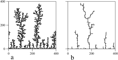
Figure 1: Typical DLD deposits which are obtained for a) weak and b) strong dipolar interactions. The deposits contain a) 12000 and b) 2000 particles.

Despite having the same fractal dimension, deposits obtained for different strengths of the dipolar interaction (equivalently, different effective temperatures) exhibit quite different structures. This situation resembles that of DLA and percolating clusters in $d=3$, namely they have the same fractal dimensions, although their geometrical structures are quite different. stanley:77:0 ; schwarzer:92:0 In this paper we characterize the deposits of dipoles further by testing a multifractal scaling of the growth probabilities $\{p_{i}\}$, where $p_{i}$ is the probability that the perimeter site $i$ is the next to be added to a cluster.

This paper is organized as follows: in section II we introduce the model of dipolar DLD and describe details of the simulations. In section III.1, the scaling exponents obtained for the density, lateral correlation function, the mean height of the upper surface and the interfacial width are compared with those of DLD. In section III.2 we present the multifractal spectra calculated for strong and weak dipolar interactions, and for several stages of growth. Finally, in section IV we summarize our findings.

II Model and Simulations Details

The model and the simulation technique are the same as in our previous works tasinkevych:04:1 ; tasinkevych:03:1 ; we briefly outline them here, and describe simulation details which allowed us to grow relatively large clusters. The simulations are performed on a two-dimensional square-lattice with lattice spacing $a$ and width $La$. The adsorbing substrate corresponds to the bottom row ($y=0$) and periodic boundary conditions are applied in the direction parallel to the substrate ($x$-direction). Particles carry a three-dimensional dipole moment of strength $\mu$ and interact with other particles through the dipolar pair-potential $\phi_{D}$:

$$\phi_{D}(1,2)=-\frac{\mu^{2}}{r^{3}_{12}}\left[3(\hat{\mbox{\boldmath$\mu$}}_{1}\cdot\hat{\mbox{\boldmath$r$}}_{12})({\hat{\mbox{\boldmath$\mu$}}_{2}}\cdot\hat{\mbox{\boldmath$r$}}_{12})-{\hat{\mbox{\boldmath$\mu$}}_{1}}\cdot{\hat{\mbox{\boldmath$\mu$}}_{2}}\right],$$ (1)

where $r_{12}=|\vec{\mbox{\boldmath$r$}}_{1}-\vec{\mbox{\boldmath$r$}}_{2}|\geq a$, $\hat{\mbox{\boldmath$r$}}_{12}=(\vec{\mbox{\boldmath$r$}}_{1}-\vec{\mbox{\boldmath$r$}}_{2})/r_{12}$, $\vec{\mbox{\boldmath$r$}}_{i}$ is a two-dimensional vector and ${\hat{\mbox{\boldmath$\mu$}}_{1}}$, ${\hat{\mbox{\boldmath$\mu$}}_{2}}$ are three-dimensional unit vectors in the direction of the dipole moments of particles 1 and 2 respectively.

Initially, a particle with random dipolar moment is introduced at the lattice site $(x_{in},H_{max}+A\,L)$, where $x_{in}$ is a random integer in the interval $[1,L]$, $H_{max}$ is the maximum height of the deposit and $A$ is a constant. The particle then diffuses by a series of jumps to nearest-neighbor lattice sites, while interacting with the particles that are already part of the deposit. Eventually, the particle either contacts the deposit (i.e., becomes a nearest-neighbor of another particle that belongs to the deposit), or attaches to the substrate (i.e., reaches the bottom of the simulation box), or moves away from the substrate. In the latter case, the particle is removed when it reaches a distance from the substrate larger than $H_{max}+2A\,L$, and a new one is introduced. Once the particle attaches to the substrate or to the deposit, its dipole relaxes along the direction of the local field created by all other particles in the deposit. In all simulations reported here we take $A=1$; larger values of $A$ have also been tested and found to give the same results, but with drastically increased computational times.

The effect of the dipolar interaction on the random walk is incorporated through a Metropolis algorithm. The interaction energy of an incoming particle with the deposit is given by $E(M,\vec{\mbox{\boldmath$r$}},{\hat{\mbox{\boldmath$\mu$}}})=\sum_{i=1}^{M}\phi_{D}(i,M+1)$, where $\vec{\mbox{\boldmath$r$}}$ denotes the particle’s position, ${\hat{\mbox{\boldmath$\mu$}}}$ is the orientation of its dipole moment and $M$ is the number of particles in the deposit. To simplify the notation, the sum over the periodic replicas of the system is omitted in the last expression. To move the particle, we select a neighboring site $\vec{\mbox{\boldmath$r$}}^{\prime}$ and a new dipole orientation ${\hat{\mbox{\boldmath$\mu$}}}^{\prime}$ randomly. This displacement is accepted with probability

$$p={\rm min}\left\{1,\exp\left[-\frac{E(M,\vec{\mbox{\boldmath$r$}}^{\prime},{\hat{\mbox{\boldmath$\mu$}}^{\prime}})-E(M,\vec{\mbox{\boldmath$r$}},\hat{\mbox{\boldmath$\mu$}})}{T^{*}}\right]\right\},$$ (2)

where $T^{*}=k_{B}Ta^{3}/\mu^{2}$ is an effective temperature inversely proportional to dipolar energy scale. In the limit $T^{*}\to 0$, only displacements which lower the energy $E$ are accepted. On the other extreme, for $T^{*}\rightarrow\infty$, all displacements are accepted and our model reduces to DLD.

One can estimate the number of calculations of $\phi_{D}$, $t$, necessary to grow a deposit of mass $M$ on a strip of width $L$ in the following way. Since each incoming particle starts its movement at a distance of order $L$ from the deposit, it takes roughly $L^{2}$ steps to reach the deposit. If there are $n$ particles in the deposit, $\phi_{D}$ has to be calculated $nL^{2}$ times. Summing this factor over $M$ particles gives $t\sim L^{2}M^{2}$. Since we have performed simulations for $L\sim 10^{3}$ and $M\sim 10^{5}$, these values roughly give $t\sim 10^{16}$, which is about 3 to 4 orders of magnitude larger than the corresponding values of the largest systems simulated in an equilibrium run of two-dimensional dipolar fluids. tavares:02:1 Therefore, to make simulations feasible we rewrite the expression for the incoming particle–deposit interaction energy in a different form. To this aim, the dipolar pair potential $\phi_{D}$, Eq. (1), is rewritten as $\phi_{D}(i,j)=\mu\vec{\mbox{\boldmath$D$}}_{ij}\cdot\hat{\mbox{\boldmath$\mu$}}_{j}$, where $\vec{\mbox{\boldmath$D$}}_{ij}$ is the dipolar field created by the particle $i$ at the site occupied by the particle $j$

$$\vec{\mbox{\boldmath$D$}}_{ij}=-\frac{\mu}{r^{3}_{ij}}\left[3(\hat{\mbox{\boldmath$\mu$}}_{i}\cdot\hat{\mbox{\boldmath$r$}}_{ij})\hat{\mbox{\boldmath$r$}}_{ij}-\hat{\mbox{\boldmath$\mu$}}_{i}\right],$$ (3)

Using Eq. (3) one can write the interaction energy between the incoming particle (which is at site $\vec{\mbox{\boldmath$r$}}_{j}$ and has a dipole orientation $\hat{\mbox{\boldmath$\mu$}}_{j}$) and a deposit formed by $M$ dipoles as

$$E(M,\vec{\mbox{\boldmath$r$}}_{j},\hat{\mbox{\boldmath$\mu$}}_{j})=\mu\vec{\mbox{\boldmath$U$}}(M,j)\cdot\hat{\mbox{\boldmath$\mu$}}_{j},$$ (4)

where $\vec{\mbox{\boldmath$U$}}(M,j)\equiv\sum_{i=1}^{M}\vec{\mbox{\boldmath$D$}}_{ij}$ (again, the sum over periodic replicas is omitted) is the dipolar field created by the deposit at site $\vec{\mbox{\boldmath$r$}}_{j}$. During simulations we store the dipolar field $\vec{\mbox{\boldmath$U$}}(j)$ at site $\vec{\mbox{\boldmath$r$}}_{j}$ together with the size of the deposit $M(j)$ for which the field $\vec{\mbox{\boldmath$U$}}$ is calculated. The particles in the deposit are ordered according to their arrival “time”. Then, the interaction energy is rewritten in the form $E(M,\vec{\mbox{\boldmath$r$}}_{j},\hat{\mbox{\boldmath$\mu$}}_{j})=\mu(\vec{\mbox{\boldmath$U$}}(j)+\sum_{i=M(j)+1}^{M}\vec{\mbox{\boldmath$D$}}_{ij})\cdot\hat{\mbox{\boldmath$\mu$}}_{j}$, which allows to reduce the number of calculations of the dipolar pair-potential from $M$ to $M-M(j)$. At the early stages of growth most of the lattice sites have not yet been visited by an incoming particle, hence $M(j)=0$. However, as the deposit grows the number of the lattice sites that have been visited more than once increases. Moreover, due to the shadowing effect, the sites close to the tips of the trees become visited more frequently, and thus the overall computation time of the dipolar energies is decreased. We have performed tests to compare the computation times for calculating the energy between the two methods. For a system of width $L\sim 10^{3}$ and $M\sim 10^{3}$ particles, the storage of the dipolar fields represents gains in computational time of about 3 orders of magnitude.

Finally, the long-range of the dipolar interaction is treated by the Ewald sum method adapted to the slab geometry of the system. tasinkevych:03:1

III Results

Simulations were carried out using four temperatures, $T^{*}=10^{-1},10^{-2},10^{-3},10^{-4}$, and four system sizes, $L=200,400,800,1600$ with 20 000, 30 000, 50 000, and 100 000 particles per deposit, respectively. Each choice of these parameters corresponds to one of the two regimes of growth. For instance, the DLA regime is never observed for the lowest temperature $T^{*}=10^{-4}$, while for $T^{*}=10^{-1}$ it is easily reached even for the smallest system size $L=200$. As we mentioned above, our previous findings suggest that the fractal dimension of the deposits $D$ is the same as for DLD even in the dipolar regime. tasinkevych:04:1 To validate this picture, we next examine the scaling behavior of the following quantities: the density of the deposit and the lateral correlation function at a given height; the mean height of the upper surface for a given number of particles; the interfacial width at a given height. All of them are global quantities that characterize the entire deposit, and which do not show any qualitative or quantitative differences between the dipolar and the DLA regimes.

III.1 The fractal dimension

A typical plot of the mean density $\rho(h)$ at a distance $h$ from the substrate has three regimes separated by two crossover heights, $h_{i}$ and $h_{s}$ (see Fig. 2). At early “times” the deposit builds up until it reaches a height $h_{i}$. Then, there appears a scaling regime during which the density decreases as a power of height, $\rho(h)\sim h^{-\alpha}$, the exponent $\alpha$ being related to the fractal dimension $D$ of the deposit by $D=2-\alpha$. meakin:84 The density stops decreasing and saturates when the lateral correlation length $\xi_{\parallel}$ reaches the size of the system $L$. Given that $\xi_{\parallel}$ grows with height as $\xi_{\parallel}\sim h^{\zeta}$, then $h_{s}\sim L^{\gamma}$, with $\gamma=\zeta^{-1}$. This behavior can be described by the scaling form

$$\rho(h,L)\sim L^{-\beta}f(h/L^{\gamma}),$$ (5)

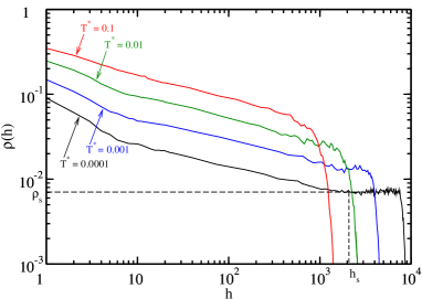
Figure 2: Mean density $\rho$ of deposits as a function of the distance $h$ from the substrate. The densities are calculated for a system-size $L=1600$ and several values of the effective temperature $T^{*}$. Beyond the crossover height $h_{s}$, the density saturates to a constant value $\rho_{s}$. The horizontal and vertical dashed-lines indicate the $\rho_{s}$ and $h_{s}$ obtained for $T^{*}=10^{-4}$.

where $f(x)$ is a scaling function with the properties: $f(x)\sim x^{-\alpha}$ for small $x$ and $f(x)\to const$ for large $x$. It is clear that $\beta=\alpha\gamma$. A linear regression between $h_{i}$ and $h_{s}$ for the largest system-size ($L=1600$) gives roughly the same scaling exponent $0.25<\alpha<0.29$, showing no systematic variation with temperature. This implies a value of the fractal dimension $1.71<D<1.75$, which is the same as for DLD. As we mentioned above, this is in contrast with a previous study, Ref. rubis, , where a continuous variation of $D$ as a function of $T^{*}$ was reported. Although several source of discrepancy are possible, differences we believe that the estimates of Ref. rubis, suffer from insufficient statistics and rather small cluster masses, that prevent the true asymptotic regime ($M\to\infty$) from being reached.

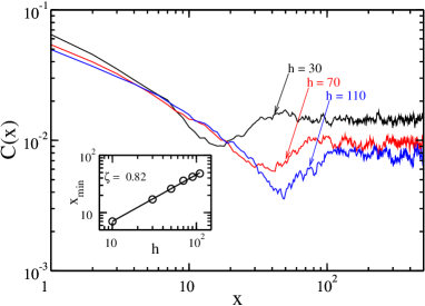
Figure 3: Lateral density-density correlation function calculated according to Eq. (6) for several distances $h$ from the substrate. The system-size is $L=1600$ and the effective temperature $T^{*}=0.1$. The position of the minimum $x_{min}$ of the correlation function as a function of $h$ is shown in the inset. $x_{min}$ scales with $h$ with a scaling exponent $\zeta\approx 0.82$.

According to Eq. (5), for $h\gg L$ the mean density attend a constant value $\rho_{s}$ that scales with the system-size as $\rho_{s}\sim L^{-\beta}$. For DLD the exponent $\beta\approx 0.33$. meakinbook This value agrees with those obtained for $T^{*}=10^{-4}$ and $T^{*}=10^{-3}$ (the only temperatures for which density saturation is neatly observed), $\beta=0.33(1)$ and $\beta=0.34(1)$, respectively. From the scaling relation $\gamma=\beta/\alpha$ one has $\gamma=1.3(1)$. An independent check of this value was carried out by calculating the height $h_{s}$ at which the density saturates and which is related to the system-size by $h_{s}\sim L^{\gamma}$. There is substantial uncertainty in the determination of $h_{s}$ and, again, we are limited to the two lowest temperatures, $T^{*}=10^{-4}$ and $10^{-3}$. For both of them $\gamma=1.30(5)$, while for DLD a value of $\gamma\approx 1.20$ has been measured.

There is a third route to the exponent $\gamma$ through the two-point lateral density-density correlation function $C(x,h)$ for horizontal cuts at a height $h$. This correlation function is defined as

$$C(x,h)=\frac{1}{L}\sum_{x^{\prime}}\sigma(x^{\prime}+x,h)\sigma(x^{\prime},h),$$ (6)

where $\sigma(x,h)$ is an occupation number which equals unity if the lattice site $(x,h)$ belongs to the deposit and zero otherwise. Fig. 3 depicts a plot of $C(x,h)$ as a function of $x$ for several heights $h$. The main feature is a pronounced minimum at $x_{min}\approx h^{\zeta}$ which can be interpreted as the mean distance between the trees at the height $h$, Ref. meakin:86:3, , and that, for DLD, scales with $h$ with an exponent $\zeta\approx 0.80-0.85$. For very large heights, the exponent $\zeta$ increases slowly with increasing height and may approach unity.meakin:86:3 Owing to poor statistics, our simulation data enables us to evaluate $\zeta$ only for $T^{*}=10^{-1}$ and $10^{-2}$, thereby extending our estimations of $\gamma$ to the entire range of available temperatures. Our results are consistent with $\zeta\approx 0.85$, equivalently $\gamma\approx 1.2$, and no significant deviation from DLD behavior is found.

Some other aspects of the morphology of the deposits have also been investigated. In our earlier work, tasinkevych:03:1 the mean height $\overline{h}$ of the upper surface $h(x)$ ($h(x)$ is defined as the maximum height of the occupied sites which are in the column $x$) was shown to scale with the number of particles $M$ (in the large-$M$ limit and for every temperature) with an effective exponent $\phi=1/(D-d+1)\approx 1.33-1.44$, which corresponds to a fractal dimension $D\approx 1.69-1.75$. In the present paper we double the number of particles of the deposits to $10^{5}$, which allows an improvement of these bounds to $D\approx 1.71-1.73$. As we wrote in Ref. tasinkevych:03:1, , had the deposits been allowed to grow only to intermediate stages (e.g., $10^{4}$ particles) an apparent variation of $D$ with $T^{*}$ would have obtained.

Owing to scale invariance, the exponent $\phi$ should coincide with the growth exponent which controls the power-law divergence of the width of the upper surface $W=\langle[h(x)-\overline{h}]^{2}\rangle^{1/2}\sim M^{\phi}$. Linear fits yield $\phi\approx 1.3-1.4$, in agreement both with our previous estimation and with the value we have measured for DLD, $\phi=1.34(2)$. The divergence of the width is cut off at the the system-size length scale, and the width reaches a saturation value $W_{sat}\sim L^{\delta}$, where the exponent $\delta$ is a conventional measure of interface roughness. Unfortunately, for every temperature saturation is barely reached only for $L=200$, whilst for the rest of sizes much bigger deposits would be necessary.

III.2 Multifractal spectrum in the dipolar and the DLA scaling regimes

We discuss hereafter the dependence of the multifractal spectrum of the growth-measure on the system size, the total number of particles, and the effective temperature.

III.2.1 General remarks

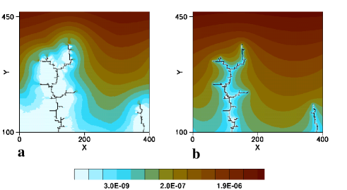
Figure 4: Iso-lines of the visit probability distribution in the vicinity of a deposit of dipoles. The probabilities are estimated numerically by using probe particles and counting the frequency of visiting of each unoccupied lattice site. The deposit contains $2000$ dipoles and has been grown at $T^{*}=10^{-4}$. In a) the strength of the dipolar interaction of the probe particles with the dipoles in the deposit corresponds to an effective temperature $T^{*}=10^{-4}$. In b) the interaction is turned off ($T^{*}=\infty$) and the probe particles follow random-walk trajectories. Dark and light regions correspond to high and low visit probabilities, respectively.

For DLA and related models, the growth probability varies sharply from site to site, changing from large values at the outer tips to very low values for the less accessible points deep within the cluster. It has been found that long-range repulsions enhance the screening effects, which leads to the formation of less branched clusters. Contrarily, long-range attractions reduce the growth probability at the cluster’s tips and lead to the formation of more compact objects. In Fig. 4.a we show the iso-lines of the visit probability distribution in the vicinity of a deposit grown at $T^{*}=10^{-4}$. To estimate the visit probabilities we use probe particles that follow biased random-walk trajectories, and register the frequency of visiting the unoccupied lattice sites. To illustrate the effects of the dipolar interaction, in Fig. 4.b we show the visit probabilities around the same deposit estimated under purely diffusive conditions ($T^{*}=\infty$), i.e. the dipolar interaction between the probe particles and the particles in the deposit has been turned off. The interaction strongly enhances screening behavior of the cluster. More perimeter sites become screened, i.e. they are characterized by smaller values of the sticking probability. On the other hand, the dipolar interaction enhances the concentration of the growth-measure at the outer sites of the cluster’s branches.

Studies of the growth probability distribution for DLA ball:90:0 ; amitrano:86 ; hayakawa:87 and related models meakin:87:1 indicate that the distribution of the growth-measure can be described in terms of a multifractal scaling model. Suppose that the boundary of a cluster of size $L$ is covered by $S(\epsilon)$ boxes of size $\epsilon$. Then, a growth measure $p(i)$ is introduced in the $i$’th box as the probability for a random-walker to land in box $i$. As mentioned above, $p(i)$ varies sharply over the cluster surface in such a way that the local growth probability density diverges at the tips and goes to zero inside the “fjords” (both behaviors are cut off at the particle length scale). To each box one can associate a singularity exponent $\alpha(i)$ via

$$p(i)\sim\Bigl{(}\frac{L}{\epsilon}\Bigr{)}^{-\alpha(i)}.$$ (7)

In what follows we keep $\epsilon$ fixed at the lower cut-off length scale, which is of one lattice unit $\epsilon\equiv 1$, and $L/\epsilon$ is varied by examining systems with different sizes $L$. The behavior of the number of boxes $N(\alpha)d\alpha$ with the scaling exponent $\alpha$ taking on a value in the interval $[\alpha,\alpha+d\alpha]$ defines the local scaling density exponent $f(\alpha)$

$$N(\alpha)\sim L^{f(\alpha)}.$$ (8)

One then introduces the scaling function $\tau(q)$ which characterizes the scaling behavior of the moments of the probability measure

$$Z(q)\equiv\sum_{i}p(i)^{q}\sim L^{-\tau(q)}.$$ (9)

Using Eqs. (7) and (8), $Z(q)$ can be written in the form

$$Z(q)\sim\int d\alpha N(\alpha)p^{q}=\int d\alpha L^{f(\alpha)-q\alpha}.$$ (10)

Evaluating this integral by saddle-point approximation leads to

$$Z(q)\sim L^{f(\alpha(q))-q\alpha(q)},$$ (11)

where the functions $\alpha(q)$ and $f(\alpha(q))$ are defined implicitly by the condition

$$\frac{df(\alpha)}{d\alpha}=q.$$ (12)

By comparing Eq. (11) with Eq. (9) the following relation is obtained

$$-\tau(q)=f(\alpha(q))-q\alpha(q).$$ (13)

The moment scaling function $\tau(q)$ is related to the family of dimensionalities $D_{q}$ introduced by Hentschel and Procaccia hp through $\tau(q)=(q-1)D_{q}$. The limit $D_{0}\equiv D\equiv\lim_{q\rightarrow 0^{+}}D_{q}$ is the fractal dimension of the cluster, and $D_{1}\equiv\lim_{q\rightarrow 1^{+}}D_{q}$ is the information dimension. For DLA, $\tau(q)$ is a non-linear function of $q$, i.e. an infinite hierarchy of exponents is required to characterize the moments of the probability measure. Some points of the $f(\alpha)$ spectrum can be related directly to the $D_{q}$: the maximum of $f$ is given by $f(\alpha(q=0))=D$, $f(\alpha(q=1))=\alpha=D_{1}$, $\alpha_{min}=D_{\infty}$, and $\alpha_{max}=D_{-\infty}$.

Usually, $\tau$ is calculated as a function of $q$ and then the multifractal spectrum $f(\alpha)$ is obtained after performing a Legendre transform. The multifractal spectra that we present here, however, are obtained through interpolation of numerical histograms, using equations (7) and (8). Because of the unknown normalization constants in these scaling relations, this method provides local growth exponent $\alpha$ and local scaling density $f(\alpha)$ up to additive corrections of order $\sim 1/\ln L$, what causes the $f$ spectra to fail to satisfy a number of important properties including data collapse, tangency of the $f=\alpha$ line and the $f(\alpha)$ curve at a single point (corresponding to $q=1$ and giving $D_{1}$), or mislocation of other representative points. Here, we shall show that taking into account these correction terms improves considerably the measured spectra (at least for low $\alpha$).

With this purpose, first note that for a finite $L$ all quantities $p,N,\alpha,f,\tau$ must carry a label $L$. We define the size dependent $\alpha_{L}$ and $f_{L}$ as following: $p_{L}\equiv L^{-\alpha_{L}}$, $N_{L}(\alpha_{L})\equiv L^{f_{L}(\alpha_{L})}$. To bring in the corrections to scaling, the integral (10) is evaluated retaining the next-order terms to give

$$Z_{L}(q)\equiv L^{-\tau_{L}(q)}\approx L^{f_{L}(\alpha_{L})-q\alpha_{L}(q)-\frac{\ln(-f_{L}^{\prime\prime})}{2\ln L}-G(L)},$$ (14)

where $G(L)=\ln[\ln L/(2\pi)]/(2\ln L)$ and $f_{L}^{\prime\prime}$ stands for the second derivative of $f_{L}$ with respect to $\alpha_{L}$. Notice that

$$\frac{df_{L}}{d\alpha_{L}}=q$$ (15)

holds. Assuming now that, to order $O(1/\ln L)$, $\tau_{L}\approx\tau$ and using Eqs. (14),(15) the following expressions can be readily derived

$$\alpha(q)=\alpha_{L}(q)+\frac{f_{L}^{\prime\prime\prime}}{2(f_{L}^{\prime\prime})^{2}\ln L},$$ (16)

$$f(\alpha)=f_{L}(\alpha_{L})+\frac{f_{L}^{\prime}f_{L}^{\prime\prime\prime}}{2(f_{L}^{\prime\prime})^{2}\ln L}-\frac{\ln(-f_{L}^{\prime\prime})}{2\ln L}-G(L).$$ (17)

Taking $\alpha_{L}$ as the independent variable, instead of $q$, then these two equations give the parametric representation of the asymptotic multifractal spectrum $f(\alpha)$ as a function of measured quantities $f_{L},\alpha_{L}$.

III.2.2 Calculation of $f_{L}(\alpha_{L})$ trough numerical histograms

The growth probabilities $p_{L}(i)$ are estimated numerically using probe particles that sample the growth measure. The probe particles follow biased random-walk trajectories in the dipolar field created by the cluster. Then $p(i)$ is calculated as $p_{L}(i)=N_{L}(i)/N_{T}$, where $N_{L}(i)$ is the number of trajectories which have terminated on the perimeter site $i$ and $N_{T}$ is the total number of trajectories (probe particles). Having estimated the growth probabilities $p_{L}(i)$, we then calculate the number of perimeter sites $N_{L}(\alpha_{L})\Delta\alpha_{L}$ with the value of $p_{L}(i)$ in the interval $[L^{-\alpha_{L}},L^{-\alpha_{L}+\Delta\alpha_{L}}]$, where $\alpha_{L}$ is defined as

$$\alpha_{L}=-\frac{\ln p_{L}(i)}{\ln L}.$$ (18)

More specifically, we calculate the histogram $N_{L}(\alpha_{L})$ from which the multifractal spectrum is obtained as

$$f_{L}(\alpha_{L})=\frac{\ln N_{L}(\alpha_{L})}{\ln L}.$$ (19)

In the calculations we choose for the width of the bin $\Delta\alpha_{L}\approx 0.15$.

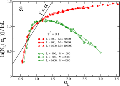
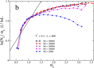
Figure 5: $f_{L}(\alpha_{L})$ spectrum of the growth probability measure for DLD of dipolar particles calculated at an effective temperature $T^{*}=0.1$ as defined in section II. This value of $T^{*}$ corresponds to the DLA scaling regime for all values of $M$ presented in the figure. $\alpha_{L}=-\ln(p_{L})/\ln L$ with $p_{L}$ being the growth measure. (a) Results obtained for system-sizes $L=400,800,800$, and deposit masses in the range $10^{3}\leq M\leq 10^{5}$. (b) demonstrates the convergence of $f_{L}(\alpha_{L})$ spectrum towards an asymptotic regime for $M>2\times 10^{4}$. We find a minimal value of the local growth exponent $\alpha_{Lmin}\approx 0.56$. The solid straight lines are given by $f_{L}=\alpha_{L}$.

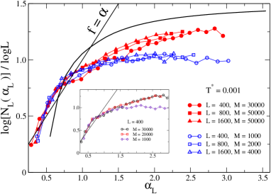
Figure 6: $f_{L}(\alpha_{L})$ spectrum of the growth probability measure for DLD of dipolar particles calculated at $T^{*}=0.001$, with $\alpha_{L}=-\ln(p_{L})/\ln L$. The results are obtained for system sizes $L=400,800,1600$, and deposit masses in the range $10^{3}\leq M\leq 5\times 10^{4}$. The solid curve schematically represents the $f_{L}(\alpha_{L})$ spectrum for $T^{*}=0.1$. The inset demonstrates the convergence of the $f_{L}(\alpha_{L})$ spectrum towards an asymptotic regime for $M>2\times 10^{4}$. The values of deposit masses $M\leq 4000$ correspond to the dipolar scaling regime; the individual trees of the deposits have the fractal dimension $D_{t}\approx 1.33$. For deposit masses $2\times 10^{4}\leq M\leq 5\times 10^{4}$ the system is in the DLA scaling regime with $D_{t}\approx 1.56$. We observe the minimal value of the local growth exponent $\alpha_{Lmin}\approx 0.36$ in both dipolar and DLA scaling regimes.

High effective-temperatures results are shown in Fig. 5. $f_{L}(\alpha_{L})$ is obtained at $T^{*}=0.1$ for deposits of size $L=400,800,1600$ and number of particles $M$ in the range $10^{3}\leq M\leq 10^{5}$. The number of probe particles used varies from $10^{8}$ for $(L,M)=(1600,10^{5})$ to $1.6\times 10^{9}$ for $(L,M)=(400,3\times 10^{4})$. The collapse of the curves shows evidence that the distribution of the measure is multifractal, with $f_{L}(\alpha_{L})$ gradually converging towards a well-defined spectrum as the deposit mass increases. An illustration that the uppermost curves are asymptotic is shown in Fig. 5b which displays data only for deposits of size $L=400$ and containing $M=$ 2000, 10000, 20000, 30000 and 50000 particles (notice the small change in $f_{L}$ when $M$ changes from 30000 to 50000). The minimal value of the local growth exponent $\alpha_{L}$ is associated with the region where the measure is most concentrated. It is found that $\alpha_{Lmin}\approx 0.56$, a value that compares favorably with measurements for DLA for $d=2$, $\alpha_{min}\approx 0.59(4)$. ball:90:0 $\alpha_{min}$ is related to the fractal dimension of the deposit $D$ through $D\geq 1+\alpha_{min}$. halsey:book This inequality is in agreement with the values of $D$ estimated by the scaling of the densities. One can identify a region of small $\alpha_{L}$’s for which the multifractal spectrum does not change with the deposit mass $M$. In particular, the value of $\alpha_{Lmin}\approx 0.56$ is the same for the biggest and the smallest deposits, ($L=1600,M=10^{5}$) and ($L=400,M=10^{3}$), what suggests that the maximum growth probability, within the considered range of $M$, does not depend on $M$. Beyond the boundary value $\alpha_{L}\approx 1.1$ there is clear mass dependence. Finally, notice that $f_{L}(\alpha_{L})$ flattens for larger values of $\alpha_{L}$. The maximum possible value of $f_{L}$, $f_{max}$, should be equal the fractal dimension $D$ of the deposit. For the DLA the maximum has been reported to be at the position $\alpha_{0}\approx 4.5$, Ref. ball:90:0, . With the Monte-Carlo technique we can not determine such small probabilities. However, one can anticipate that $f_{max}$ is not far from the expected value $D$.

Low effective temperatures results are displayed in Fig. 6. $f_{L}(\alpha_{L})$ is calculated at $T^{*}=10^{-3}$ for both the initial and late stages of growth (small and large $M$), the number of probe particles varying from $7.9\times 10^{6}$ for $(L,M)=(1600,5\times 10^{4})$ to $5\times 10^{7}$ for $(L,M)=(400,3\times 10^{4})$. The initial stages of growth correspond to the dipolar regime, with the deposits containing $M=1000,2000,4000$ particles for $L=400,800,1600$, respectively. At the late stages of growth ($M=30000,50000,50000$ for $L=400,800,1600$ respectively), the DLA regime has been attained, as described in section IIIA. The inset of Fig. 6 demonstrates the convergence of $f_{L}(\alpha_{L})$ towards the asymptotic behavior which is reached at $M>20000$. Again, like in the case $T^{*}=0.1$, a region of small $\alpha_{L}$’s can be identified where the multifractal spectra does not depend on $M$. In fact, in both regimes we obtain a value of $\alpha_{Lmin}\approx 0.36$, which is considerably lower than the corresponding value obtained for $T^{*}=0.1$. The turning point separating $M$-dependent from $M$-independent behavior is located at $\alpha_{L}\approx 1.35$. Beyond this point good data collapse is still observed for the dipolar regime, whereas the collapse of the curves is not impressive after the crossover to the DLA regime has taken place. We shall see below how to amend this shortcoming. The changes in the shape of the $f_{L}$-spectrum as $M$ grows can be interpreted as an increase in the fractal dimension of the screened parts of the deposit, but for the studied range of $\alpha_{L}$’s, $f_{L}$ still stays well below the $T^{*}=0.1$ curve. According to the picture developed in section III.1, the maximum values of $f_{L}$ should equal $D\approx 1.71$. The figure suggests a further increase in $f_{L}$ if more probe particles are used to estimate the growth probabilities. Although no conclusive statements can be made regarding this point, we shall see in the next subsection that it is expected that the large $\alpha_{L}$ parts of the spectra shift upwards once corrections to scaling have been included.

Lastly, the elongated appearance of the trees in the dipolar regime resembles that observed in the initial stages of deposits grown at high temperatures in the DLA regime. Our data show, however, that the multifractal structure of the dipolar regime is clearly different from those of the initial stages of growth of deposits at higher temperatures, even if the fractal dimensions are similar.

III.2.3 Corrected spectra

When the multifractal measure possesses a continuous spectrum, the straight line $y=\alpha$ is tangent to the $f(\alpha)$ curve at $f(\alpha)=\alpha$. halsey:88:0 This general behavior is not seen in the hitherto shown spectra because they have been obtained through numerical histograms. Hence, the scaling relations expressed by Eqs. (7), (8) provide the local growth exponent $\alpha$ and the local scaling density $f(\alpha)$ up to additive constants $\sim 1/\ln L$. This is the reason why the curves shown in the Figs. 5, 6, instead of being tangent to the line $y=\alpha$, intersect it. The multifractal spectra presented in Refs. meakin:87:1, ; meakin:86:1, ; schwarzer:92:0, were also calculated as numerical histograms, and display the same behavior.

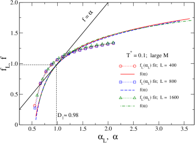
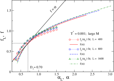
Figure 7: Corrected spectra $f(\alpha)$ calculated according to the Eqs. (16),(17) for $T^{*}=0.1$, upper panel, and $T^{*}=0.001$, lower panel. The numerical curves $f_{L}(\alpha_{L})$ are fitted to the function $a_{0}+a_{1}\exp(a_{2}\alpha_{L}^{a_{3}})+a_{4}\ln(\alpha_{L})$. The symbols represents the fitted functions, and the lines – corrected spectra $f(\alpha)$. For $T^{*}=0.1$ the numerical data only in the range $\alpha_{Lmin}\leq\alpha_{L}\leq 2.1$, and for $T^{*}=0.001$ in $\alpha_{Lmin}\leq\alpha_{L}\leq 1.5$, are fitted.

From a more physical point of view, $f(\alpha)=\alpha$ is a turning point that separates regions of the spectrum corresponding to high (small $\alpha$) and low (large $\alpha$) growth probabilities. Moreover, the subset satisfying $f(\alpha)=\alpha$ has a fractal dimension equal to the information dimension $D_{1}$ of the multifractal formalism introduced by Hentschel and Procaccia. hp The particles in this subset carry almost all the growth probability, in such a way that $D_{1}$ is the fractal dimension of the active zone, i.e. the unscreened surface. The identification of $D_{1}$ from Figs. 5, 6 is troublesome since there is no tangency at $f_{L}=\alpha_{L}$. The use of the corrected expressions (16) and (17) is therefore called for, but their application immediately poses the problem of computing up to third order numerical derivatives from noisy, scarce simulation data. We therefore resorted to fitting to the simulation data several functional forms. In Fig. 7 results for the corrected $f(\alpha)$ are shown for the particular choice of the fitting function $a_{0}+a_{1}\exp(a_{2}\alpha_{L}^{a_{3}})+a_{4}\ln(\alpha_{L})$. The numerical data are fitted only for the values of $\alpha_{L}$ in the range $\alpha_{Lmin}\leq\alpha_{L}\leq 2.1$ for $T^{*}=0.1$, and $\alpha_{Lmin}\leq\alpha_{L}\leq 1.5$ for $T^{*}=0.001$. For the larger values of $\alpha_{L}$ there is a big uncertainty in the numerical data, thus those parts of the $f_{L}(\alpha_{L})$ curves are excluded from this particular fitting procedure. We stress that the Fig. 7 is shown only as a qualitative illustration of the effects of the corrections terms in equations (16) and (17). In particular, the tangency property is restored in every case, while data collapse is preserved. Estimating $D_{1}$ as the value of $f$ where the $f$-curve has unit slope we obtain $D_{1}\approx 0.98$ for $T=0.1$, which is close to the exact result $D_{1}=1$ for DLA. makarov With decreasing $T^{*}$ we observe the decrease of $D_{1}$, namely we find $D_{1}\approx 0.84$ and $D_{1}\approx 0.70$ for $T^{*}=0.01$ (the corresponding figure is not shown) and $T^{*}=0.001$ respectively. Other functional forms yield very similar results.

The corrected spectra have other interesting features as compared to the uncorrected ones. At this point, however, the discussion has to be kept at a qualitative level since at the extreme values of $\alpha_{L}$ one faces two different numerical problems: i) on approaching $\alpha_{min}$ the derivatives of any order of “true” spectra $f$ diverge; ii) on the other hand, large $\alpha_{L}$ values correspond to data with poor statistics. Some general observations can nevertheless be made. There is strong indication that, upon incorporation of the corrections terms: i) the part of the $f_{L}$-curve corresponding to large $\alpha_{L}$ shifts upwards for every temperature; ii) data collapse emerges for $T^{*}=0.001$. In particular, for the values of $\alpha\approx 3.0$, $f(\alpha)$ takes similar values for both values of $T^{*}$, a result consistent with the interpretation that the fractal dimension does not depend on the effective temperature. Note also that a remarkable improvement in data-collapse can be observed for the case $T^{*}=0.001$ and large $M$. Finally, there is a slight tendency for $\alpha_{min}$ to move to the right. For $T^{*}=0.1$ the corrected value gets even closer to its DLA value whereas for $T^{*}=0.001$ it keeps at $\alpha_{min}\approx 0.4$. We stress that on the whole this same behavior carries over to other fitting choices. We also calculate the corrections to the measured $f_{L}(\alpha_{L})$ spectrum in the dipolar scaling regime $(T^{*}=0.001)$ and small values of $M)$. As expected we get the same $\alpha_{min}$ and $D_{1}$ as for large $M$, but no concluding evidence that $D$ is going to be the same.

According to the Turkevich-Scher conjecture $D=1+\alpha_{min}$, turkevich:85:0 such behavior of $\alpha_{min}$ would be in contradiction with the fact that $D$ does not change with effective temperature (as concluded in section III.1). The above mentioned relation between $D$ and $\alpha_{min}$ is obtained using implicitly the assumption that the most extremal sites of the clusters, or tips, are the most active ones, i.e. $\alpha_{tip}=\alpha_{min}$. We have checked the location of the sites with maximum growth probability in the clusters of simulations, and found that they often do not coincide with the clusters tips. Thus, $\alpha_{tip}\geq\alpha_{min}$ and the more general relation $D\geq 1+\alpha_{min}$, Ref. halsey:book, , applies in this case.

IV Conclusions

The diffusion-limited deposition of magnetic particles shows a crossover between two regimes, with a crossover size that sensitively depends on the temperature. At the early stages of growth both the fractal dimension of the trees $D_{t}$ and their size-distribution, as given by the exponent $\tau$, are temperature dependent and have significantly smaller values as compared with those of pure DLD (dipolar regime). As the size of the trees exceeds the crossover value $s^{*}$ the diffusion-driven DLA scaling regime emerges. In this regime $D_{t}$ and $\tau$ have the same values as in DLD. tasinkevych:04:1 Here, we have provided evidences that the fractal dimension of the entire deposit remains constant as the deposition proceeds. This has been done by analyzing the density profile of the deposit, the lateral correlation function, and the mean height and the width of the upper surface. It ensues that $D_{t}$ and $\tau$ conspire so as to give a fixed value of $D$.

Multifractal analysis shows that, for each value of the interaction parameter and at each stage of growth, the normalized distribution of growth probabilities can be scaled onto a single curve using the same scaling form as in DLD thereby providing the $f(\alpha)$-spectrum. The features of the $f(\alpha)$ spectra allows us to distinguish the structure of the deposits at high and low temperature (see Fig. 1). We have found that $\alpha_{min}$ decreases significantly with decreasing temperature, revealing that the concentration of the growth probability becomes more and more marked when dipolar interactions are increased. Likewise, the fractal dimension of the active zone $D_{1}$ decreases with decreasing temperature, meaning that for low temperatures less sites are involved in the growth of the deposit. As a consequence, and since $D_{1}$ and $\alpha_{min}$ do not depend on the stage of growth, the presence of dipolar interactions reveals in the structure of the deposits by increasing further the probability of growth at “hotter” sites and by originating less dense deposits. On the other hand, the $f(\alpha)$ spectra at late stages of growth suggest that the fractal dimension of the deposits does not depend on temperature (or dipolar interaction), corroborating our previous results. However, our findings also indicate that the $f(\alpha)$-spectra in the high- and low-temperature DLA scaling regimes are different.

The multifractal spectrum in the dipolar regime (low temperature at the early stages of growth) is clearly different from that in the initial stages of growth at high temperature, thus providing evidence that these two situations have to be held distinct. The $f(\alpha)$ spectrum obtained for the dipolar regime was, however, not accurate enough to confirm that the fractal dimension of the deposits in this regime is approximately equal to that of later stages of growth.

In a more general perspective, this work shows that the information dimension $D_{1}$ and the scaling exponent $\alpha_{min}$ are much easier to determine through a numerical measurement of the $f(\alpha)$ spectrum then the fractal dimension $D$, provided that the corrections of Eqs. (16) and (17) are taken into account. In fact, the low $\alpha$ part of a spectrum can be obtained with good statistics using small systems (see Figs. 5 and 6). Therefore, our work suggests that the effect of interactions in DLA (or DLD) deposits could be more easily studied through $D_{1}$ and $\alpha_{min}$.

- (1) T. A. Witten and L. M. Sander, Phys. Rev. Lett. 47, 1400 (1981).
- (2) P. Meakin, Fractals, scaling and growth far from equilibrium , Cambridge University Press, Cambridge (1998).
- (3) P. Meakin, Phys. Rev. A, 27, 2616 (1983).
- (4) P. Meakin, H. E. Stanley, A. Coniglio, and T. A. Witten Phys. Rev. A 32, 2364 (1985).
- (5) T. C. Halsey, P. Meakin, and I. Procaccia, Phys. Rev. Lett. 56, 854 (1986).
- (6) P. Meakin, J. Chem. Phys. 79, 2426 (1983).
- (7) P. Meakin and M. Muthukumar, J. Chem. Phys. 91, 3212 (1989).
- (8) N. Vandewalle and M. Ausloos, Phys. Rev E 51, 597 (1995).
- (9) E. Somfai, R. C. Ball, N. E. Bowler, and L. M. Sander, Physica A 325, 19 (2003).
- (10) R. Pastor-Satorras and J.M. Rubí, Phys. Rev. E 51, 5994 (1995); Prog. Colloid. Polym. Sci. 110, 29 (1998); J. Magn. Magn. Mater. 221, 124 (2000).
- (11) P.M. Mors, R. Botet, and R. Jullien, J. Phys. A 20, L975 (1987).
- (12) G. Helgesen, A.T. Skjeltorp, P.M. Mors, R. Botet, and R. Jullien, Phys. Rev. Lett. 61, 1736 (1988).
- (13) F. de los Santos, J. M. Tavares, M. Tasinkevych, and M. M. Telo da Gama, Phys. Rev. E 69, 061406 (2004).
- (14) P. Meakin and F. Family, Phys. Rev. A 34, 2558 (1986).
- (15) Z. Rácz and T. Vicsek, Phys. Rev. Lett. 51, 2382 (1983).
- (16) H. E. Stanley, J. Phys. A: Math. Gen. 10, L211 (1977).
- (17) S. Schwarzer, M. Wolf, S. Havlin, P. Meakin, and H. E. Stanley, Phys. Rev. A 46, R3016 (1992).
- (18) F. de los Santos, M. Tasinkevych, J.M. Tavares, and P.I.C. Teixeira, J. Phys.: Condens. Matter 15, S1291 (2003).
- (19) J. M. Tavares, J. J. Weis, and M. M. Telo da Gama, Phys. Rev. E (2002).
- (20) P. Meakin, Phys. Rev. B 30, 4207 (1984).
- (21) Notice that in rubis : i) the dynamics of the dipoles is different: the orientation of their dipolar moments does not change between two consecutive steps, but after each accepted step it relaxes along the total field at the arrival lattice site; ii) deposition occurs on a single growth site rather than on a line (slab geometry); iii) 2d dipoles satisfying 3d electrostatics are used.
- (22) R.C. Ball and O.R. Spivack, J. Phys. A: Math. Gen. 23, 5295 (1990).
- (23) C. Amitrano, A. Coniglio, and F. di Liberto, Phys. Rev. Lett. 57, 1016 (1986).
- (24) Y. Hayakawa, S. Sato, and M. Matsushita, Phys. Rev. A 36, 1963 (1987).
- (25) P. Meakin, Phys. Rev. A 35, 2234 (1987).
- (26) H .G. E. Hentschel and I. Procaccia, Physica 8D, 435 (1983).
- (27) T. C. Halsey in Fractals’ Physical Origin and Properties, edited by L. Pietronero (Plenum Press, New York, 1989), p.205.
- (28) T. C. Halsey, Phys. Rev. A 38 , 4789 (1988).
- (29) P. Meakin, Phys. Rev. A 34, 710 (1986).
- (30) N. G. Makarov, Proc. Lon. Math. Soc. 51, 369 (1985).
- (31) L. Turkevich and H. Scher, Phys. Rev. Lett. 55, 1026 (1985); Phys. Rev. A 33, 786 (1986).